Báo cáo y học: "Directed cell migration in the presence of obstacles" doc
Bạn đang xem bản rút gọn của tài liệu. Xem và tải ngay bản đầy đủ của tài liệu tại đây (344.92 KB, 12 trang )
BioMed Central
Page 1 of 12
(page number not for citation purposes)
Theoretical Biology and Medical
Modelling
Open Access
Research
Directed cell migration in the presence of obstacles
Ramon Grima*
1,2
Address:
1
Indiana University School of Informatics and Biocomplexity Institute, Bloomington, IN 47406, USA and
2
Institute for Mathematical
Sciences, Imperial College, London SW7 2PG, UK
Email: Ramon Grima* -
* Corresponding author
Abstract
Background: Chemotactic movement is a common feature of many cells and microscopic
organisms. In vivo, chemotactic cells have to follow a chemotactic gradient and simultaneously avoid
the numerous obstacles present in their migratory path towards the chemotactic source. It is not
clear how cells detect and avoid obstacles, in particular whether they need a specialized biological
mechanism to do so.
Results: We propose that cells can sense the presence of obstacles and avoid them because
obstacles interfere with the chemical field. We build a model to test this hypothesis and find that
this naturally enables efficient at-a-distance sensing to be achieved with no need for a specific and
active obstacle-sensing mechanism. We find that (i) the efficiency of obstacle avoidance depends
strongly on whether the chemotactic chemical reacts or remains unabsorbed at the obstacle
surface. In particular, it is found that chemotactic cells generally avoid absorbing barriers much
more easily than non-absorbing ones. (ii) The typically low noise in a cell's motion hinders the ability
to avoid obstacles. We also derive an expression estimating the typical distance traveled by
chemotactic cells in a 3D random distribution of obstacles before capture; this is a measure of the
distance over which chemotaxis is viable as a means of directing cells from one point to another in
vivo.
Conclusion: Chemotactic cells, in many cases, can avoid obstacles by simply following the spatially
perturbed chemical gradients around obstacles. It is thus unlikely that they have developed
specialized mechanisms to cope with environments having low to moderate concentrations of
obstacles.
Background
Directed cell motion is a common feature of many cells
and micro-organisms; this movement can be induced by a
number of factors including light (phototaxis), gravity
(gravitotaxis) and various chemicals (chemotaxis). The
last of these is the most pervasive natural form of taxis.
The bacteria Escherichia coli and Salmonella typhimurium,
the slime mould Dictyostelium discoideum, and neutrophils
[1] are a few of the many well studied examples of chem-
otactic life-forms. Chemotaxis involves the detection of a
local chemical gradient and the subsequent movement of
the organism up (positive chemotaxis) or down (negative
chemotaxis) the gradient. For example, Dictyostelium dis-
coideum follows trails of folic acid secreted by its food
source, bacteria, so as to track and eventually capture
them [2]. Another example is the chemotaxis of neu-
Published: 16 January 2007
Theoretical Biology and Medical Modelling 2007, 4:2 doi:10.1186/1742-4682-4-2
Received: 2 October 2006
Accepted: 16 January 2007
This article is available from: />© 2007 Grima; licensee BioMed Central Ltd.
This is an Open Access article distributed under the terms of the Creative Commons Attribution License ( />),
which permits unrestricted use, distribution, and reproduction in any medium, provided the original work is properly cited.
Theoretical Biology and Medical Modelling 2007, 4:2 />Page 2 of 12
(page number not for citation purposes)
trophils to gradients of C5a released at a wound site – the
neutrophils kill bacteria and decontaminate the wound
from foreign debris.
Over the years, various aspects of chemotactic behavior
have been studied from both an experimental and a theo-
retical point of view (e.g. [3-9]). In this article we study the
efficiency of chemotaxis in achieving controlled cell
migration to specific sites in the heterogeneous environ-
ments typical of in vivo conditions. Current models of
chemotactic movement do not directly address such
issues. Typically, these models simulate the interaction of
cells with each other and ignore the physical environment
in which the movement is occurring, e.g. non-chemotactic
cells and foreign debris in the path of the migrating chem-
otactic cells.
Since environmental heterogeneity occurs on a scale com-
parable to that of individual cells, macroscopic contin-
uum models (usually based on the Keller-Segel model
[10]) of cell movement are not appropriate to answer the
above questions. Rather, one requires an approach involv-
ing an individual-based model (IBM) of cell movement.
In this article we construct a minimal IBM of chemotactic
cell movement in an obstacle-ridden environment. Our
aim is to understand the efficiency of chemotaxis in such
conditions and whether additional biological mecha-
nisms (e.g. an active obstacle-sensing mechanism) are
needed to ensure that the chemotactic cell reaches the
source of the chemical to which it is sensitive. A few spe-
cialized mechanisms of this type are known, for example
the case of axon guidance [11], in which a combination of
chemoattractants and chemorepellents secreted by other
cells in the environment guide the axons along very spe-
cific routes to generate precise patterns of neuronal wir-
ing. However, this is not the general case, particularly for
free-swimming cellular organisms, which may be simply
involved in following chemoattractant left by their prey
and thus have no apparent foreknowledge of any obsta-
cles in their path. These are the cases we shall treat in this
study.
In the next section, we first review and summarize some
basic facts about cell movement that follow from the
underlying biology and physics. On the basis of this infor-
mation, we build the simplest (deterministic) realistic
model of cell movement and by means of an analytical
analysis we use it to understand the movement of a chem-
otactic cell in the presence of a single obstacle. This will
clearly prove that cells can naturally sense and avoid
obstacles by simply following the chemical gradient and
that in many cases they do not require additional special-
ized mechanisms. We study the efficiency of obstacle
avoidance as a function of the cell-obstacle size ratio and
the type of obstacle: obstacles can either not interact with
the chemotactic chemical or act as a sink. Next, we study
the effect of noise on the probability of the cell being cap-
tured by an obstacle, and finally we conclude by extend-
ing our analysis to the case of a multi-obstacle
environment. This leads to an expression for the distance
over which chemotaxis is viable as a means of directing
cells from one point to another in vivo.
Chemotactic motion of a cell around an obstacle
In this section we study the motion of a chemotactic cell
when a single obstacle is placed in its migratory path
towards the chemoattractant source. There are two types
of chemotactic sensing: (i) Spatial sensing, in which a cell
compares the chemoattractant concentration at two dif-
ferent points on its body. This mechanism is, for example,
used by the slime mould and neutrophils. (ii) Temporal
sensing, in which a cell compares the concentration at two
different times. This is used by flagellated bacteria such as
Escherichia coli and Salmonella typhimurium. There is a
process related to chemotaxis, called chemokinesis, in
which the speed of cell movement is determined by the
absolute value of the local concentration but the cell does
not actually orient [12]. In this article we shall be con-
cerned exclusively with chemotaxis via a spatial sensing
mechanism.
The non-absorbing obstacle case
Consider a spherical chemotactic cell of radius a in a uni-
form chemical gradient of magnitude ∇ C = g ; the gra-
dient is chosen to be directed along the positive z-axis in
a right-handed coordinate system. Note that C denotes
the chemical field. If the cell is positively chemotactic, its
movement is up the gradient in a direction parallel to the
z-axis. Next we introduce a spherical obstacle of radius R
centered at the origin. The setup is illustrated in Fig. 1. The
question we are interested in is: Can the cell avoid the
obstacle just by following the chemical gradient or does it
need an additional biological mechanism ? Note that the
cell and the obstacle are assumed to be in a fluid at rest;
the obstacle is stationary relative to the fluid and immo-
bile; only the cell moves. We wish to make absolutely
clear that this is not the classical case of a cell carried by a
moving fluid past a stationary obstacle. The cell's move-
ment is only due to its response to external chemotactic
stimuli.
Now we proceed to construct a simple physical model to
answer the above question. First we summarize some
basic facts about cell movement, which follow from the
underlying physics and/or biology:
1. Inertial effects are insignificant to the cell's movement.
This follows from the fact that cells and micro-organisms
ˆ
z
Theoretical Biology and Medical Modelling 2007, 4:2 />Page 3 of 12
(page number not for citation purposes)
typically exist in low-Reynold's number environments
[13,14].
2. The cell is able to resolve the chemical gradient along its
body (a spatial sensing mechanism). It is well known that
many eukaryotic cells [12] and even some types of bacte-
ria [15] have this ability.
3. The chemotactic force on a cell is directly proportional
to the chemical gradient across its body. This is implicity
assumed in many models of chemotaxis, such as the Kel-
ler-Segel model [10] and its discrete counterpart [8]. This
approximation is satisfactory if the chemical concentra-
tion is not too large; this follows theoretically from a con-
sideration of receptor kinetics (see [16] for example).
It thus follows that the cell's movement can be modeled
via an over-damped equation of the form:
c
(t) =
α
∇ C (x
c
(t), t), (1)
where x
c
(t) is the position of the cell's center of mass at
time t and
α
is a positive constant measuring the cell's
chemotactic sensitivity. Note that the above equation fol-
lows from Newton's second law when viscous drag domi-
nates over the inertial force (i.e. small Reynold's number).
For the moment we ignore stochastic contributions to the
cell's trajectory; effects stemming from intrinsic noise will
be studied in a later section. Note that in our mathemati-
cal formulation, the cell's motion is determined by the
chemical gradient in the center of the cell. This is a good
approximation to the gradient across their bodies (which
is what is actually measured) provided the cell is not too
large. Using the gradient at the center of the cell will ena-
ble a mathematical analysis to be conducted that is not
possible otherwise; however, in our ensuing numerical
simulations, we will compare results using both the gradi-
ent at the cell's center and that calculated as a concentra-
tion difference across the cell's body.
Next we need to specify equations for the chemical field.
Two main considerations determine these equations:
1. The interaction of the chemical with the obstacle's sur-
face. The object can be impermeable to the chemical, i.e.
the chemical bounces off the obstacle's surface without
any appreciable absorption, or it can interact with the
chemical.
2. The diffusive relaxation time of the chemical field will
determine whether the field sensed by the cell is in steady-
state. For the sake of mathematical simplification, we
shall assume that it is. This is physically justified in two
cases: (i) the chemical field is set up well before cell migra-
tion starts. This is thought to be the case, for example, in
some morphogenetic processes [17], where cells follow a
chemical pre-pattern laid at an earlier time, (ii) If both the
set up of the field and cell migration occur at the same
time, then steady-state can only be achieved if the time
taken to set up the field over the obstacle region by diffu-
sion, Δt
D
~R
2
/D
c
, is much less than the time taken for the
cell to traverse the same region, Δt
c
~R/
α
g. Note that D
c
is
the chemical diffusion coefficient and that the last two
expressions are correct up to some multiplicative con-
stant. Thus the steady state assumption is valid if the ine-
quality
α
gR/D
c
<< 1 is approximately satisfied.
Given these considerations and assuming isotropy of the
medium in which cell movement occurs (i.e. the chemical
diffusion coefficient is not a function of space but a con-
stant), the chemical field is described by Laplace's equa-
tion ∇
2
C (r,
θ
,
φ
) = 0, with boundary condition: ∇ C = g
in the limit r → ∞. We note that there may be many sit-
uations in vivo when the isotropy assumption does not
hold; we shall ignore such complications, though many of
the results we shall derive probably also translate to cases
where the properties of the medium change very slowly
over the region in which the obstacle is located. In this
subsection we shall treat the case of a non-absorbing
obstacle, which follows by imposing the surface no-flux
boundary condition ∇
r
C (r = R) = 0. In the next subsec-
x
ˆ
z
Graphical representation of the system under investigationFigure 1
Graphical representation of the system under inves-
tigation. A spherical obstacle of radius R is placed in the
path of a chemotactic cell of radius a. The chemical gradient
far away from the obstacle is constant and in the z-axis direc-
tion. The y-axis is out of the page. The angle
θ
is measured
anticlockwise from the positive z-axis.
z
x
r
θ
direction of chemotactic gradient
Cell
Obstacle
R
2a
Theoretical Biology and Medical Modelling 2007, 4:2 />Page 4 of 12
(page number not for citation purposes)
tion we shall consider the opposite case of an absorbing
obstacle.
Now that we have specified equations for both cell move-
ment and the chemical field, we proceed to determine the
cell's spatial trajectory. The obstacle's physical presence
significantly distorts and modifies the chemical field in its
surroundings and thus alters the cell's chemotactic move-
ment. Adopting spherical coordinates, we solve Laplace's
equation with the specified boundary conditions. Since
the chemical gradient for large r is along the z-axis, the
solution has to possess azimuthal symmetry (i.e. symmet-
ric with respect to rotations in
φ
); then the general solu-
tion to Laplace's equation is:
where P
l
are Legendre polynomials, A
l
and B
l
are constants
to be determined from the boundary conditions and l is
an integer. Imposing the boundary conditions, the chem-
ical field in the space around the spherical obstacle is
given by:
where C
0
is the concentration for position coordinates
θ
=
π
/2.
Now we proceed to find the cell trajectory in the vicinity
of the obstacle. Substituting Eq.(2) in Eq.(l), after some
simple algebraic manipulation we obtain:
where r
c
and
θ
c
are the position coordinates of the cell.
Thus the equation of the cell's path is given by:
which upon integrating gives:
This equation describes the spatial trajectory of the chem-
otactic cell. Note that d is the x position of the cell when it
is still far away from the obstacle's influence. This is anal-
ogous to the impact parameter in the physics of scattering
[18]. The trajectory is independent of the magnitude of
the chemical gradient g, and of the chemotactic sensitivity
α
. Typical cell trajectories are illustrated in Fig. 2(a).
Cr Ar Br p
l
l
l
l
l
i
,, cos ,
θφ θ
()
=+
()
()
−+
()
=
∞
∑
1
0
Cr C gr
R
r
,cos,
θθ
()
=+ +
⎛
⎝
⎜
⎜
⎞
⎠
⎟
⎟
()
0
3
3
1
2
2
dr
dt
g
R
r
c
c
c
=−
⎛
⎝
⎜
⎜
⎞
⎠
⎟
⎟
()
αθ
cos ,13
3
3
d
dt
g
r
R
r
cc
c
c
θαθ
=− +
⎛
⎝
⎜
⎜
⎞
⎠
⎟
⎟
()
sin
,1
2
4
3
3
dr
d
rRr
Rr
c
c
cc c
c
θ
θ
=
−−
()
+
()
()
cot /
/
,
1
12
5
33
33
r
rR
d
c
c
c
33
12
6
−
⎛
⎝
⎜
⎜
⎞
⎠
⎟
⎟
=
()
/
sin
.
θ
Typical trajectories of the center of mass of a chemotactic cell with a non-absorbing object of unit radius placed in its pathFigure 2
Typical trajectories of the center of mass of a chemo-
tactic cell with a non-absorbing object of unit radius
placed in its path. (a) The equation describing these paths
is given by Eq. (6). Initially the cells are placed at z = -3 with d
= 0.25, 0.5, 0.75,1,1.25,1.5. Note that here d corresponds to
the x position of the cell at z = -3. In this diagram we do not
consider any mechanical interaction between the cell and the
sphere. (b) Same as (a) but now the cell radius is fixed at 0.1
and we allow interactions (i.e. attachment upon contact)
between the cell and the sphere. Note that cells with d d 0.5
do NOT make it past the obstacle. This is because the cap-
ture radius, as given by Eq.(7), for a cell with radius 0.1 and
an obstacle of unit radius is equal to 0.55.
-3
-2
-1
0
1
2
3
-3 -2 -1 0 1 2 3
z
x
-3
-2
-1
0
1
2
3
-3 -2 -1 0 1 2 3
x
z
(a)
(b)
Theoretical Biology and Medical Modelling 2007, 4:2 />Page 5 of 12
(page number not for citation purposes)
Thus we conclude that spatial perturbations of the chem-
ical field in an object's vicinity, due to its physical pres-
ence, enable a chemotactic cell to avoid the obstacle
simply by following the modified gradient. In many cases,
there is NO need for an additional mechanism to sense
and avoid the obstacle. This is not always the case since a
cell can only directly avoid the obstacle if the distance of
closest approach r
min
is greater than the sum of the obsta-
cle's and the cell's radii, i.e. r
min
≥ a + R.
A proper discussion of obstacle avoidance requires knowl-
edge of the exact interaction between the cell and the
obstacle upon mechanical contact. This is a subject of cur-
rent research; generally, cells adhere to each other, to the
extracellular matrix and to other biopolymers via various
types of cell adhesion molecules. The strength of this
adhesion depends sensitively on the specific type of cells
and the obstacles under consideration. The dynamics of
cell movement very close to the obstacle surface are also
influenced by short-range hydrodynamic interactions
between the two. In the interest of having an analytically
tractable model, we shall ignore hydrodynamic interac-
tions and assume irreversible adhesion of a cell to an
obstacle upon mechanical contact. Our ensuing discus-
sions regarding cell capture are based on this assumption.
We note that since cells do not generally adhere perma-
nently to obstacles, the estimates we shall derive for the
probability of cell capture (which is a measure of the effi-
ciency of chemotactic obstacle avoidance) are to be
viewed as upper bounds for the real case. Further discus-
sion of these assumptions is deferred to the last section of
this article.
We shall now quantify the efficiency of chemotactic obsta-
cle avoidance. A convenient quantity to calculate is the
capture radius r
cap
. For a cell of radius a moving in a
straight line trajectory towards a spherical obstacle of
radius R, the capture radius is r
cap
= a + R. However, the
streamline-like trajectories induced by spatial perturba-
tions in the chemical field imply that r
cap
< a + R. To calcu-
late the actual capture radius, consider the following
argument. From Eq. (5) it can be seen that the closest dis-
tance of approach r
min
occurs at
θ
=
π
/2; the capture radius
r
cap
is then given by the value of d for which r
min
= a + R.
From Eq.(6), we then have:
where
δ
= a/R. The physical relevance of the capture radius
can be appreciated by the following simple experiment,
which is illustrated in Fig. 2(b). Suppose that at time t = 0,
a cell is randomly positioned on a circle in the x-y plane
with center (x = 0, y = 0, z = -3) and radius R'. We repeat
this experiment a large number of times, each time noting
whether the cell is eventually captured. We would observe
that cells that were initially within a radius d = r
cap
are cap-
tured by the obstacle; cells initially within the annulus
defined by the radius range r
cap
<d <R' would, however,
chemotactically avoid the obstacle. Another measure of
the efficiency of chemotactic obstacle avoidance is as fol-
lows. Consider again the experiment depicted in Fig. 2b.
with the difference that R' = a + R. What is the probability
that the cells will be able to avoid the obstacle? In general,
this quantity is simply given by the expression: P
cap
=
π
/
π
(a + R)
2
. Note that if we had to ignore the spatial
perturbation of the field, then P
cap
= 1. Otherwise, we
have:
Thus P
cap
< 1 and it decreases monotonically as a function
of
δ
= a/R. For cells with radius a t R/4, the capture prob-
ability is greater than 0.5, so obstacle avoidance by simply
following chemotactic gradients is not efficient for cells
larger than this. We note that the total capture probability
should actually be calculated in the limit R' → ∞. How-
ever, since cells initially within an annulus defined by the
radius range d > a + R always avoid the obstacle, P
cap
given
by Eq. (8) has to be equal to P
cap
calculated in the limit of
infinitely large R'.
We now investigate the apparent geometric similarity of
the chemotactic cell trajectories around a non-absorbing
obstacle (Fig. 2) to the streamlines of an incompressible
and inviscid fluid around a spherical object. Consider the
irrotational flow of an incompressible and inviscid fluid
past a spherical object [19]. If u is the fluid velocity, then
irrotational flow implies that ∇ × u = 0; this can also be
expressed in terms of a scalar function,
φ
, as u = ∇
φ
. Fur-
thermore, incompressibility implies ∇·u = 0. Combining
the irrotational and incompressibility conditions, we
obtain Laplace's equation ∇
2
φ
= 0.
φ
is thus commonly
referred to as the velocity potential. Since the normal com-
ponent of the fluid velocity u has to be zero at the obsta-
cle's surface, we have the boundary condition n·∇
φ
= 0.
The movement of a chemotactic cell in an external uni-
form chemical field perturbed by an obstacle is thus math-
ematically analogous: u ≡
c
and
φ
≡ C. The mathematical
form of the chemotactic cell trajectories is therefore
exactly the same as that describing streamlines of fluid
rR
cap
=
+
()
−
+
()
11
1
7
3
δ
δ
,
r
cap
2
P
cap
=
+
()
−
+
()
()
11
1
8
3
3
δ
δ
.
x
Theoretical Biology and Medical Modelling 2007, 4:2 />Page 6 of 12
(page number not for citation purposes)
flow around an obstacle. This has one important implica-
tion: It is not possible to distinguish between the case of a
chemotactic cell following a gradient around an obstacle
in a stationary fluid and a non-chemotactic cell dragged
past a stationary obstacle by a moving fluid. This equiva-
lence is strictly speaking only valid for the case of a chem-
otactic cell with velocity directly proportional to the
chemical gradient. As previously mentioned, this assump-
tion is correct if the absolute value of the chemical con-
centration is small. More generally, the chemotactic
velocity is a non-linear function of the chemical gradient
and the chemical concentration, examples being a loga-
rithmic response due to sensory adaptation (see [20] and
references therein) and more complicated responses [9].
The equivalence may also be broken by temporal delays
between changes in the chemical stimulus and the ensu-
ing chemotactic response. As we shall see in the next sec-
tion, it also breaks down if the obstacle absorbs some of
the chemotactic chemical at its surface.
The absorbing obstacle case
In this subsection we explore the effect of the obstacle's
absorption properties on the cell trajectories and the cap-
ture probability. In all our previous discussions we have
assumed that the obstacle does not absorb any chemical.
However, in a number of cases the chemotactic chemical
might take part in reactions on the obstacle's surface,
meaning that some of the molecules will be sequestered
upon reaching the surface. In this section we consider the
opposite case to that in the previous section: the obstacle
is assumed to be a perfect sink for the chemical, sequester-
ing every molecule that reaches its surface. The chemical
field around such an obstacle is obtained by solving
Laplace's equation ∇
2
C (r,
θ
,
φ
) = 0 with boundary condi-
tions: ∇ C = g in the limit r → ∞ and C (r = R) = 0. The
chemical field is then described by an equation of the
form:
where C
0
is the concentration for position coordinates (r
→ ∞,
θ
=
π
/2). As in the previous subsection, we obtain
the equations for dr
c
/dt and d
θ
c
/dt and divide to obtain:
Direct solution of this equation is a non-trivial task. A
more straightforward approach involves using Stoke's
stream function,
ψ
, which is a common method for solv-
ing hydrodynamic problems [19]. The trajectory of a cell
corresponds to
ψ
= k, where the constant k is determined
by the cell's position when it is far away from the obstacle.
The stream function in a plane is determined from the
equations:
∂
ψ
/
∂
r = - sin
θ
∂
C/
∂θ
and
∂ψ
/
∂θ
= r
2
sin
θ
∂
C/
∂
r. Solving these simple equations for
ψ
, equating this
resultant expression to k (this is determined by assuming
that the initial position of the cell is (x, z) = (d, e)) and
substituting r = r
c
and
θ
=
θ
c
, we obtain the final equation
for the trajectory of the cell:
which satisfies Eq.(10), as can be verified by direct substi-
tution. Contrary to the case in which the obstacle does not
absorb any chemical, we notice in this case that the geo-
metrical form of the cell path depends on the magnitude
of the chemical gradient g, the chemotactic sensitivity
α
,
the absolute value of the chemical concentration C
0
and
the initial distance of the cell along the z-axis e. Typical
cell trajectories are illustrated in Fig. 3. Note the consider-
able difference from the cell trajectories typical of the non-
absorbing case (see Fig. 2a).
ˆ
z
Cr C
R
r
gr
R
r
,cos,
θθ
()
=−
⎛
⎝
⎜
⎞
⎠
⎟
+−
⎛
⎝
⎜
⎜
⎞
⎠
⎟
⎟
()
0
3
3
11 9
dr
d
CR r gr R r
gRr
c
c
ccc c
cc
θ
αθ
αθ
=−
++
()
−
()
()
0
333
33
12
1
10
/cos /
sin /
.
r
R
r
CR
g
d
C
gd e
cc
c
c
22
3
3
0
2
0
22
1
2
22
11sin
cos
,
θ
θ
α
α
+
⎛
⎝
⎜
⎜
⎞
⎠
⎟
⎟
−=−
+
()
Re
Typical trajectories of the center of mass of a chemotactic cell with a perfectly absorbing object of unit radius placed in its pathFigure 3
Typical trajectories of the center of mass of a chemo-
tactic cell with a perfectly absorbing object of unit
radius placed in its path. All parameters with the excep-
tion of C
0
are set to unity. The value of C
0
is equal to 10. The
equation describing these paths is given by Eq. (11). Initially
the cells are placed at z = -5 with d = 0.001, 0.5 – 4.5 in 0.5
step intervals. In this diagram we do not consider any
mechanical interaction between the cell and the sphere.
0
1
2
3
4
5
6
7
-4 -2 0 2 4
x
z
Theoretical Biology and Medical Modelling 2007, 4:2 />Page 7 of 12
(page number not for citation purposes)
Several observations can be made: (i) the trajectories are
not symmetrical about the obstacle, i.e. when it passes the
obstacle, a cell suffers a permanent change in its trajectory;
(ii) through-out its motion past the obstacle, a cell never
comes very close, even when d is very small; (iii) the effect
of the obstacle on the cell's movement is appreciable even
at large distances r >> R.
These observations can all be explained by considering
the obstacle-perturbed field Eq.(9). Consider a cell that is
initially placed very close to the z-axis, i.e. d is very small.
The force it experiences in the z-direction is proportional
to the concentration gradient in this direction, a graph of
which is shown in Fig. 4(b). The cell initially approaches
the obstacle's surface but stops moving towards it when
the force becomes zero. In the region close to the obsta-
cle's surface, the gradient is negative and thus this region
is inaccessible to the cell. The gradient is negative because
at the obstacle's surface the concentration is zero, a condi-
tion dictated by the obstacle being an idealized sink. Note
that this was not the case when the obstacle was non-
absorbent, in which case the gradient was always positive
and became zero only at the surface (see Fig. 4(a)). This
explains observation (ii) above.
We now use this argument to calculate the minimum
radius required for a cell to be captured and hence deduce
the corresponding capture probability. Note that the latter
quantity refers to the experiment introduced in the previ-
ous section. The cells passing the closest to the obstacle
are the ones initially close to the z-axis, i.e. d is small. For
such cells the distance of closest approach r
min
occurs at
θ
Ӎ
π
. This can be most easily demonstrated by substituting
Eq. (11) with d = 0 in Eq. (10) with the R.H.S equal to
zero; solving for
θ
gives the angle at which the cell
approaches the obstacle most closely. Thus for cells with
small d, the distance of closest approach, r
min
, is given by
the z position (along the line x = y = 0) at which the gra-
dient in the z-direction becomes zero, which satisfies the
equation:
Then a cell is captured if its radius a satisfies the condition
a + R ≥ r
min
. Cells with a radius smaller than the critical
radius a = r
min
- R will not be captured, irrespective of d. For
cells larger than the critical radius, capture may occur if d
is small enough, but not in general. Thus the capture
probability is zero for cells smaller than the critical radius
and non-zero otherwise. This differs from the case of a
non-absorbing obstacle, in which the capture probability
is always greater than zero irrespective of cell size (see Fig.
5). For the parameter values used in Fig. 5, the above
equation predicts r
min
= 3.06, which implies a ≥ 2.06 for
capture, a fact verified by the simulation data in the figure.
Note also that the simulations (see Fig. 5) indicate that the
theoretical results for both the absorbing and the non-
absorbing obstacle cases, which were derived on the basis
of a cell sensing the gradient in its center, are also qualita-
tively reproduced if cells sense the gradient across their
bodies.
Observation (iii) can be explained by noting that the per-
turbation in the chemical field, Eq.(9), decays much more
slowly for long distances (decays as 1/r) than it does for
the non-absorbing case (decays as 1/r
3
). Observation (i) is
explained by the fact that after a cell passes the obstacle it
does not experience a force pulling it back towards the
obstacle; this is because the chemical gradient in the x-
direction at any point in space always points away from
the obstacle, since the concentration at the surface is zero.
The effect of noise on the capture probability
In this section we study the effect of noise on the obstacle
avoiding abilities of chemotactic cells. In the deterministic
case, the cell's motion was completely determined by the
local chemical gradient. We now relax this condition by
requiring that the cell's motion is partly determined by
intrinsic noise and partly by the gradient. The cell's
motion will be modeled as a random walk, characterized
by a cell diffusion coefficient D, biased in the direction of
increasing gradient.
r
CR
g
r
R
g
min min
3
0
3
2
012−+=
()
.
Graph of the concentration C versus distance z on the line x = y = 0Figure 4
Graph of the concentration C versus distance z on
the line x = y = 0. for (a) a non-absorbing obstacle (b) an
absorbing obstacle. The parameter values are all set to unity
with the exception of C
0
, which has value 10. Note that the
obstacle has its center at the origin and thus a boundary at z
= -1.
0
1
2
3
4
5
6
7
8
9
-5 -4.5 -4 -3.5 -3 -2.5 -2 -1.5 -1
(a)
(b)
C
z
Theoretical Biology and Medical Modelling 2007, 4:2 />Page 8 of 12
(page number not for citation purposes)
The stochastic description is in all aspects similar to the
deterministic one, with the exception that the equation
describing the cell's motion has an extra noise term:
c
(t) =
α
∇
C (x
c
(t), t) +
ξ
(t). (13)
This is a Langevin equation [21]. The stochastic variable
ξ
is white noise defined through the relations: Ό
ξ
a
(t) = 0
and Ό
ξ
a
(t)
ξ
b
(t') = 2 D
δ
a,b
δ
(t - t'), where a and b refer to
the spatial components of the noise vectors and D is the
cell's diffusion coefficient. Note that the angled brackets
denote the statistical average. For convenience, the carte-
sian components of the noise vector will be denoted as
ξ
(t) = (
ξ
x
(t),
ξ
y
(t),
ξ
z
(t)). Assuming that the obstacle is
non-absorbing, the concentration field C is as given by
Eq.(2). As before, we switch to a description in spherical
polar coordinates. The equations of motion for the chem-
otactic cell are then:
where
γ
(
θ
c
,
φ
c
, t) = sin
θ
c
cos
φ
c
ξ
x
(t) + sin
θ
c
sin
φ
c
ξ
y
(t) + cos
θ
c
ξ
z
(t). (17)
In contrast to the deterministic case, the cell's movement
is not restricted to a plane and is dependent on the mag-
nitude of the chemical gradient g. Note that we recover the
deterministic case by setting the noise to zero, which
implies
θ
c
= constant (motion in a plane) and independ-
ence of the cell's trajectory from the gradient (this follows
by dividing Eq. (14) by Eq. (15) as done in the previous
section). A standard general method for analyzing sto-
chastic differential equations involves a small noise
expansion [21] about the deterministic solution. This
method rests on the assumption that a deterministic
explicit solution is known, i.e. r
c
(t) = f (t),
θ
c
(t) = g (t),
φ
c
(t) = h (t). No such explicit solutions can be obtained in
our case; this can most easily be seen by using Eq.(6) to
derive an expression for cos
θ
c
, which is then substituted
in Eq.(3) to obtain a first-order non-linear differential
equation for r
c
(t). Hence the above equations do not lend
themselves easily to analysis; it is not generally possible to
derive equations for the trajectory, capture radius and cap-
ture probability for the stochastic case. Thus our investiga-
tion of the role and effect of noise on the dynamics will be
solely through numerical simulation.
We probe the system's stochastic behavior by measuring
the capture probability P
cap
as a function of the cell diffu-
sion coefficient D, which is a measure of the noise
strength. To measure the capture probability the following
setup is used. A spherical obstacle of radius R = 1 is placed
x
dr
dt
g
R
r
t
c
c
c
cc
=+
⎛
⎝
⎜
⎜
⎞
⎠
⎟
⎟
+
()
()
αθ γθφ
cos , , ,114
3
3
d
dt
g
r
R
r
tt
r
cc
c
c
ccc z
c
θαθ
θθφ ξ
=− +
⎛
⎝
⎜
⎜
⎞
⎠
⎟
⎟
+
()
−
()
sin
cos , ,
si
1
2
3
3
γ
nn
,
θ
c
15
()
d
dt r
t
t
ccc
cc
y
x
c
φθθ
φ
ξ
ξ
φ
=
()
−
()
⎛
⎝
⎜
⎜
⎞
⎠
⎟
⎟
()
cos cot
cos cot
,16
Graph of the capture probability P
cap
versus the ratio of the cell to obstacle radius a/RFigure 5
Graph of the capture probability P
cap
versus the ratio
of the cell to obstacle radius a/R. for (a) a non-absorbing
obstacle (b) a perfectly absorbing obstacle. The parameter
values are all set to unity with the exception of C
0
, which has
value 10. Notice that for the second case only cells larger
than a certain critical size are captured. The data for these
plots were obtained from theory (green) and simulations
(blue, red) for (a). The blue curve is computed using the gra-
dient in the middle of the cell and the red curve is computed
using the gradient across its body. The data for (b) are from
simulations only, with the green curve representing data with
the central gradient and the blue curve representing data
using the gradient across the cell's body.
0
0.1
0.2
0.3
0.4
0.5
0.6
0.7
0.8
0.9
0 0.2 0.4 0.6 0.8 1
0
0.1
0.2
0.3
0.4
0.5
0.6
0.7
0.8
0.9
0 1 2 3 4 5
P
cap
a / R
a / R
P
cap
(a)
(b)
Theoretical Biology and Medical Modelling 2007, 4:2 />Page 9 of 12
(page number not for citation purposes)
at the origin as in Fig. 1. At t = 0, a cell of radius a is ran-
domly placed on a circle in the x-y plane of radius a + R
and center coordinates x = 0; y = 0; z = -3. The cell motion
is determined by numerically integrating Eq. (13). At each
time step, the algorithm computes the new cell position
and checks whether the cell has come into contact with
the obstacle. If this condition is found to be true then the
simulation stops and a counter is increased by one. If the
condition is false then the program keeps running until
either the condition becomes true or the cell reaches the
plane z = 3. Note that the counter is not reset to zero after
the program finishes. This simple program is run 5 × 10
4
times; the capture probability is then given by the value of
the counter divided by 5 × 10
4
. Note that stopping the
simulation when the plane z = 3 is reached is an arbitrary
choice, initially made to mirror the initial position sym-
metrically; we found that changing the stopping value of
z generally has minor effects on P
cap
except when the cell
diffusion coefficient is substantially large. This is because
in the latter case the cell has a significant probability of
being captured after passing the obstacle (by moving
against the gradient), which does not happen at small dif-
fusion coefficients. The larger the stopping value of z, the
higher the probability that this will occur. The results of
our simulations are shown in Fig. 6. Two general observa-
tions can be made: (i) For any given D, the capture prob-
ability is proportional to the cell radius. This is expected,
(ii) P
cap
peaks at a particular value of D. This peak behavior
is clearly distinguishable and relevant only for small val-
ues of the cell radius, a d 0.4.
This last observation requires some explanation. The peak
in the capture probability separates two distinct regimes
of dynamical behavior: (i) the chemotaxis-dominated
regime in which cells strongly follow the chemical gradi-
ent (ii) the diffusion-dominated regime in which the cell
behavior is mostly stochastic and only weakly determined
by the chemotactic gradients. The two regimes are approx-
imately determined by the two timescales:
τ
c
~L/
α
g and
τ
d
~L
2
/6 D, where L = 2 R is the obstacle's diameter. Cell
movement is mainly by chemotaxis when
τ
c
<<
τ
d
(chem-
otaxis-dominated regime) and principally by diffusion
when
τ
d
<<
τ
c
(diffusion-dominated regime). This is indeed
conceptually parallel to the advection-dominated (high
Peclet number) and diffusion-dominated (low Peclet
number) regimes in models of chemical transport in flu-
ids. Whereas the cell's x-position is approximately limited
to the range x ∈ [-(a + R), a + R] for very small diffusion,
the range is much greater for large diffusion. Of course the
larger the range, the smaller the probability of the cell
being captured. The range is dictated by the magnitude of
the fluctuations in the cell's position, which grows
roughly as ; hence in the diffusion-dominated regime
we expect the probability of capture to decrease with
increasing diffusion coefficient.
What remains to be explained is the increase in capture
probability with noise in the chemotaxis-dominated
regime. Here, a cell roughly follows the trajectories of the
deterministic case. Consider two different and non-inter-
acting cells: cell 1 is placed just inside the capture radius d
= r
cap
-
δ
x and cell 2 just outside of the capture radius d =
r
cap
+
δ
x. Capture, if it occurs, will happen at or near the
obstacle's equator (
θ
=
π
/2) since this is the distance of
closest approach. Owing to noise fluctuations, cells 1 and
2 may switch positions in the course of their path towards
the obstacle. If it was equally probable for the cells to
switch positions, then the capture probability would not
change from the deterministic case. However, this is not
the case: cell 1 in the course of its path towards the obsta-
cle's equator passes closer to the obstacle's surface than
cell 2, implying that the probability of cell 1 leaving the
capture volume is less than the probability of cell 2 enter-
ing it. This qualitatively explains the increase in capture
probability with increasing noise in the chemotaxis-dom-
inated regime.
A rough measure of P
cap
for low noise can be obtained by
the following argument. In the deterministic case, the cap-
ture radius is determined by the initial cell position
(denoted d in the previous section), for which the distance
D
Graph showing the variation of the capture probability P
cap
with the cell diffusion coefficient DFigure 6
Graph showing the variation of the capture probabil-
ity P
cap
with the cell diffusion coefficient D. The varia-
tion is shown for different values of the cell radius a. The
obstacle is non-absorbing and has unit radius. The parameter
values are all set to unity.
0.2
0.3
0.4
0.5
0.6
0.7
0.8
0.9
1e-06 1e-05 0.0001 0.001 0.01 0.1 1 10
a=0.1
a=0.2
a=0.4
a=0.8
P
D
cap
Theoretical Biology and Medical Modelling 2007, 4:2 />Page 10 of 12
(page number not for citation purposes)
of closest approach equals the sum of the cell and obstacle
radii, i.e. r
min
= a + R. The addition of noise to the system
enables a cell to be captured for r
min
> a + R. Consider a cell
with an initial position that places it outside the determin-
istic capture radius. By the time a cell has arrived at the
obstacle's equator (where the distance of closest approach
occurs), the fluctuations in its position are roughly
δ
x =
= , implying that r
min
~(a + R) +
. The distance L
0
is the length of the cell's path
from its initial position to the point at which it reaches the
obstacle's equator; this is roughly equal to 3 in our case.
Given the new r
min
, one can compute P
cap
as previously
done for the deterministic case. Note that this rough cal-
culation overestimates P
cap
; this is because we have not
taken into account the fact that some cells initially within
the capture radius will escape capture, as explained in the
previous paragraph. The stochastic correction to r
min
is rel-
atively more significant for small cell radii than for larger
ones; this qualitatively explains why there is hardly any
change in P
cap
for a t 0.4 over four orders of magnitude of
noise, but a marked change for smaller values of a.
In our simulations we have kept the obstacle radius R
fixed at unity. In general we find that the effect of increas-
ing R (all other factors constant) is qualitatively the same
as decreasing the cell radius a. However, note that whereas
in the deterministic case the behavior was determined
exclusively by the ratio a/R, this is not the case here, except
in the limit of low noise.
We have also investigated the effect of noise on the
motion of a cell around a perfectly absorbing obstacle. As
for the non-absorbing case, we find that there are two dis-
tinct regimes: chemotaxis-dominated and diffusion-dom-
inated. For the first regime, the capture probability
increases with noise strength, whereas in the second the
opposite effect occurs. The reasons are the same as for the
non-absorbing case. One peculiarity of the absorbing case
is the following. For the deterministic case, the capture
probability is zero for cells smaller than a critical radius
and greater than zero otherwise (see Fig. 5b). Low noise
lowers this critical threshold. It is also generally the case
that noise has less effect on the capture probabilities for
the absorbing than for the non-absorbing obstacle case.
This is because cells passing around absorbing obstacles
tend to remain further from the obstacle than if the obsta-
cle was non-absorbing, as is clear from the trajectories
illustrated in Fig. 2 and Fig. 3.
We finish this section by noting that if we had to consider
the effect of noise on the capture probability of a cell in
the presence of many obstacles, then the situation is con-
siderably more complex. In particular, the results of this
section would only hold in the more general case if the
concentration of obstacles was small.
Efficiency of chemotaxis in a multi-obstacle space
Under in vivo conditions, chemotactic cells have to navi-
gate to the chemotactic source by avoiding various kinds
of obstacles. The question we want to address in this sec-
tion is: what is the mean free path of a chemotactic cell
under in vivo conditions? In other words, over what spatial
distances is chemotaxis an efficient process for guiding
cells from one location to another?
To answer such a question, the most general scenario to
consider would be a random 3D distribution of obstacles.
Let the obstacles be of the non-absorbing kind and let the
mean obstacle separation be significantly greater than the
obstacle radius. The latter assumption guarantees that the
field around any given obstacle is decoupled from the
effects of nearby ones. This assumption will enable us to
use the results derived in previous sections. We restrict
ourselves to deterministic cell movement.
The average distance traveled by a cell before permanent
capture is conceptually the same as the mean free path of
a gas molecule, which is usually estimated from kinetic
theory [22]. Consider a very thin slab of space of cross-sec-
tional area L
2
and infinitesimal width dz, in which obsta-
cles are randomly distributed with a number density
ρ
o
.
The effective cross-section for capture by each obstacle, is
π
, where r
cap
is the capture radius as defined by Eq. (7).
Then the obstacles present a total capture area equal to
(
π
)
ρ
o
L
2
dz; thus it follows that the probability of a cell
being captured as it passes through the slab of space is
equal to:
Setting P = 1 gives us the typical distance traveled before
capture,
λ
:
where
δ
= a/R. An interesting consequence of this formula
is that for small cells (a << R),
λ
is proportional to 1/R. If
we did not take account of the spatial perturbations in the
2Dt
δ
2
0
DL g/
α
2
0
DL g/
α
r
cap
2
r
cap
2
P
rLdz
L
rdz
cap o
cap o
=
()
=
()
()
πρ
πρ
22
2
2
18.
λ
πρ
δ
πρ δ
==
+
+
()
−
⎡
⎣
⎢
⎤
⎦
⎥
()
11
11
19
2
2
3
ocap
o
r
R
,
Theoretical Biology and Medical Modelling 2007, 4:2 />Page 11 of 12
(page number not for citation purposes)
chemical field due to the obstacle, the capture radius r
cap
would simply be equal to R, implying that
λ
∝ 1/R
2
. It is
also easy to show that since the fractional change in the
number density of cells after they have passed through the
slab is proportional to P, the spatial distribution of cells
has to be exponential:
ρ
c
∝ e
-z/
λ
, where
ρ
c
is the number
density of cells.
Note that the above estimates are only valid for low obsta-
cle number density. It is not possible to derive
λ
for the
stochastic case since there are no explicit expressions for
the capture radius. For the absorbing obstacle case, r
cap
= 0
for cells smaller than a critical size and greater than zero
otherwise. This implies that
λ
= ∞ for cells below the crit-
ical size and finite otherwise.
Conclusion
The main aim of this study was to investigate how cells
avoid obstacles in in vivo environments: do they need a
special obstacle-sensing mechanism to follow a chemo-
tactic signal efficiently in an obstacle-ridden spatial
region? In this article, we have investigated by means of a
simple model, the movement of a chemotactic cell when
an obstacle is placed in its direct path of motion towards
a chemotactic source. The physical presence of the obsta-
cle perturbs the chemical field near its surface. A cell on a
direct collision course with the obstacle can in many cases
avoid it by simply following the perturbed chemical gra-
dient in its vicinity. The ability to do so depends strongly
on two factors: the cell-to-obstacle size ratio and the
chemical absorbing properties of the obstacle.
If the obstacle does not absorb any chemical, then cells of
all sizes have a non-zero probability of avoiding it. The
probability is very small for cells comparable in size to the
obstacle and only appreciable for cells with radii smaller
than approximately a quarter of the obstacle's radius.
If the obstacle sequesters chemical molecules at its sur-
face, then the situation is very different. In this case, cells
smaller than a certain critical size always avoid the obsta-
cle. This critical size can be comparable to or even larger
than the obstacle size, meaning that even large cells on a
direct collision path with the obstacle can easily avoid it
by simply following the perturbed gradient.
For both cases, we find that noise (as measured by the cell
diffusion coefficient) decreases the chances of a cell avoid-
ing an obstacle if the dynamics are chemotaxis-dominated
and increases its chances if noise-dominated. By chemo-
taxis-dominated we mean that the cell's velocity is prima-
rily determined by the chemical gradient, whereas noise-
dominated means that the cell's motion appears to be
similar to a random walk, though it is weakly biased in the
direction of the chemical gradient. Interestingly, a cell is
least successful in escaping an obstacle when chemotaxis
and noise contribute approximately equally to its motion.
Note that although large noise enhances the cell's obstacle
avoidance ability, it simultaneously reduces its ability to
follow the direction dictated by the chemical gradient.
Thus, overall, cells with low noise, i.e. small diffusion
coefficients, are most advantaged in avoiding obstacles
and successfully following the chemical pre-pattern.
We also find that the trajectories of cells with linear chem-
otactic responses around non-absorbing obstacles in a
static fluid are exactly of the same mathematical form as
the streamlines of a non-viscous fluid past a static obsta-
cle. This means that the two cases are physically indistin-
guishable. This equivalence does not hold for the case of
an absorbing obstacle, or for non-linear or delayed chem-
otactic responses.
Throughout our study we have implicitly ignored short-
range hydrodynamic interactions between the cell and the
obstacle and simply modeled the interaction of the two by
assuming that a cell irreversibly adheres to an obstacle
upon mechanical contact. The fate of a real cell when it
touches some obstacle depends on the complex interfacial
forces between the two. A possible scenario is that upon
encounter with an obstacle, a cell temporarily adheres,
but intrinsic noise in its motion will eventually enable it
to leave the obstacle's surface. However, note that low
noise can only lead to temporary and frequent sticking
and unsticking of the cell about the point of its first cap-
ture, so a captured cell will take a significantly long time
to pass the obstacle in such circumstances. Chemical gra-
dients are set up for some finite period of time; if the time
required for a cell to pass an obstacle is comparable to or
longer than this time, than the cell would effectively be
counted as captured. Thus our conclusion is that for low
noise, reversible adhesion (temporary capture) leads to
the same results we derived in this article for irreversible
adhesion (permanent capture).
In conclusion we have shown, by considering the under-
lying physics, that chemotactic cells, in many cases can
avoid obstacles by simply following the spatially per-
turbed chemical gradients around them. This may explain
why specialized biological mechanisms for avoiding
obstacles are only known for a handful of cells and organ-
isms.
Acknowledgements
The author would like to thank Edward Flach for helpful discussions and
gratefully acknowledges support by a grant from the Faculty Research Sup-
port Program from the OVPR, Indiana University (Bloomington Campus).
References
1. Alberts B, Johnshon A, Lewis J, Raff M, Roberts K, Walter P: Molecular
Biology of the Cell New York: Garland Science; 2002.
Publish with BioMed Central and every
scientist can read your work free of charge
"BioMed Central will be the most significant development for
disseminating the results of biomedical research in our lifetime."
Sir Paul Nurse, Cancer Research UK
Your research papers will be:
available free of charge to the entire biomedical community
peer reviewed and published immediately upon acceptance
cited in PubMed and archived on PubMed Central
yours — you keep the copyright
Submit your manuscript here:
/>BioMedcentral
Theoretical Biology and Medical Modelling 2007, 4:2 />Page 12 of 12
(page number not for citation purposes)
2. Armitage JP, Lackie JM: Biology of the Chemotactic Response Cambridge:
Cambridge University Press; 1990.
3. Berg HC, Purcell EM: Physics of Chemoreception. Biophys J 1977,
20:193-219.
4. Beyer T, Meyer-Hermann M, Soff G: A possible role of chemo-
taxis in germinal center formation. Int Immunol 2002,
14:1369-1381.
5. Grima R: Strong Coupling Dynamics of a Multicellular Chem-
otactic system. Phys Rev Lett 2005, 95:128103.
6. Jiang Y, Levine H, Glazier JA: Possible cooperation of differential
adhesion and chemotaxis in mound formation of Dictyostel-
ium. Biophys J 1998, 75:2615-2625.
7. Maree AFM, Hogeweg P: How amoeboids self-organize into a
fruiting body: Multicellular coordination in Dictyostelium
discoideum. Proc Natl Acad Sci USA 2001, 98:3879-3883.
8. Newman T, Grima R: Many-body theory of cell-cell interac-
tions. Phys Rev E 2004, 70:051916.
9. Rivero MA, Tranquillo RT, Buetnner HM, Lauffenburger DA: Trans-
port models for chemotactic cell populations based on indi-
vidual cell behavior. Chem Eng Sci 1989, 44:2881-2897.
10. Keller EF, Segel LA: Model for Chemotaxis. J Theor Biol 1971,
30:225-234.
11. Dickson B: Molecular Mechanisms of Axon Guidance. Science
2002, 298:1959-1964.
12. Bray D: Cell Movements: From molecules to motility Garland Publishing;
2001.
13. Berg HC: Random Walks in Biology Princeton: Princeton University
Press; 1993.
14. Purcell EM: Life at low Reynold's number. Amer J Phys 1977,
45:3-11.
15. Thar R, Kuhl M:
Bacteria are not too small for spatial sensing
of chemical gradients: An experimental evidence. Proc Natl
Acad Sci USA 2003, 100:5748-5753.
16. Othmer HG, Stevens A: Aggregation, Blowup and Collapse:
The ABC's of Taxis in Reinforced Random Walks. Siam J Appl
Math 1997, 57:1044-1081.
17. Wolpert L, Beddington R, Jessel T, Lawrence P, Meyerowitz E, Smith
J: Principles of Development Oxford: Oxford University Press; 2001.
18. Krane KS: Introductory Nuclear Physics Wiley; 1987.
19. Lamb H: Hydrodynamics Cambridge: Cambridge University Press;
1997.
20. Grima R: Phase transitions and superuniversality in the
dynamics of a self-driven particle. Phys Rev E 2006, 74:011125.
21. Gardiner CW: Handbook of Stochastic Methods Berlin: Springer; 1995.
22. Mortimer RG: Physical Chemistry San Diego: Harcourt University
Press; 2000.