Báo cáo y học: " Theoretical size distribution of fossil taxa: analysis of a null model" ppsx
Bạn đang xem bản rút gọn của tài liệu. Xem và tải ngay bản đầy đủ của tài liệu tại đây (398.07 KB, 12 trang )
BioMed Central
Page 1 of 12
(page number not for citation purposes)
Theoretical Biology and Medical
Modelling
Open Access
Research
Theoretical size distribution of fossil taxa: analysis of a null model
William J Reed*
1
and Barry D Hughes
2
Address:
1
Department of Mathematics and Statistics, University of Victoria, Victoria, British Columbia V8W 3P4, Canada and
2
Department of
Mathematics and Statistics, University of Melbourne, Parkville, Victoria 3010, Australia
Email: William J Reed* - ; Barry D Hughes -
* Corresponding author
Abstract
Background: This article deals with the theoretical size distribution (of number of sub-taxa) of a
fossil taxon arising from a simple null model of macroevolution.
Model: New species arise through speciations occurring independently and at random at a fixed
probability rate, while extinctions either occur independently and at random (background
extinctions) or cataclysmically. In addition new genera are assumed to arise through speciations of
a very radical nature, again assumed to occur independently and at random at a fixed probability
rate.
Conclusion: The size distributions of the pioneering genus (following a cataclysm) and of derived
genera are determined. Also the distribution of the number of genera is considered along with a
comparison of the probability of a monospecific genus with that of a monogeneric family.
Background
Mathematical modelling of the evolution of lineages goes
back at least to Yule[1] who developed the eponymous
Yule process (homogeneous pure birth process) in which
speciations occur independently and at random. Yule's
model did not include extinctions per se, because he
believed that they resulted only from cataclysmic events.
This issue was discussed at greater length by Raup[2], who
distinguished between background and episodic extinc-
tions. Raup started from a homomogeneous birth-and-
death process model (in which background extinctions
occur, like speciations, independently and at random) for
which he presented mathematical results, and described
more complex models of extinction including episodic
extinctions and a mixture of episodic and background
extinctions. However he gave no mathematical results for
these models. Stoyan[3] considered a time in-homogene-
ous birth-and death process, in which speciation and
background extinction rates varied with time, based on
the idea that younger paraclades have higher speciation
rates, while older ones have higher background extinction
rates.
There has been considerable discussion (e.g. Raup[2];
Patzkowsky[4]; Przeworski and Wall[5]) about the suita-
bility of the null birth-and-death process model (with
constant birth and death rates) as a macroevolutionary
model of species diversification. In order to truly assess
the validity of such a model it is necessary to have a full
understanding of its properties which can then be com-
pared with the fossil record. Specifically analysis is needed
to generate hypotheses, which can be tested against avail-
able data. To date such an analysis is incomplete, relying
on the partial analytic results of Raup[2] and the simula-
tion results of Patzkowsky[4] and Przeworski and Wall[5].
Published: 22 March 2007
Theoretical Biology and Medical Modelling 2007, 4:12 doi:10.1186/1742-4682-4-12
Received: 11 December 2006
Accepted: 22 March 2007
This article is available from: />© 2007 Reed and Hughes; licensee BioMed Central Ltd.
This is an Open Access article distributed under the terms of the Creative Commons Attribution License ( />),
which permits unrestricted use, distribution, and reproduction in any medium, provided the original work is properly cited.
Theoretical Biology and Medical Modelling 2007, 4:12 />Page 2 of 12
(page number not for citation purposes)
Analytic results are clearly superior to simulation ones. In
particular with analytic results for the size distribution of
a clade one can fit the model via a multinomial likeli-
hood, using observed size distributions, and thence test
the adequacy of the underlying birth-and-death model
using a statistical goodness-of-fit test. In addition analytic
results are preferable to simulation ones, in that it is much
easier to interpret a parametric formula than a collection
of simulation results; and one does not have to distin-
guish between sampling variation due to a finite number
of runs (noise) and signal.
It is the purpose of this paper to conduct a more thorough
analysis of the birth-and-death model than that previosly
carried out by Raup[2]. In particular we obtain results for
size distributions of taxa and probabilities of monotypic
taxa. In this paper we confine attention to obtaining ana-
lytic results and defer actual fitting and testing of the fit,
using observed fossil data, to a future paper.
We develop the mathematical model presented by
Raup[2] (and used in simulations by the above authors)
to include the possibility of episodic, cataclysmic extinc-
tions in which complete lineages are destroyed. We con-
sider a hiearchy of models, which can include both
cataclysmic and background extinctions of species and
examine the resulting size distributions of extinct genera.
We start (following section), as did Yule, by considering
cataclysmic extinction only. Furthermore like Patz-
kowsky[4] and Przeworski and Wall [5], we assume that at
any time an existing species can split, yielding a new spe-
cies so radically different from existing ones that it
becomes the founding member of a new genus. Thus we
assume that the probability of a new genus being formed
in an infinitesimal interval (t, t + dt) is proportional to the
total number of species in existence at time t. We derive
results for the size distribution of extinct genera.
In the third and fourth sections we do the same assuming
only background extinctions (but no cataclysmic extinc-
tion); and both cataclysmic and background extinctions
(although the results here are limited). The fifth section is
devoted to the distribution of the number of genera
derived from the pioneering species and in the final sec-
tion the probability of a monotypic genus is compared
with that of a monogeneric family.
Cataclysmic extinctions only
Yule[1] considered the evolution of a genus begining with
one species at time t = 0, which thenceforth evolves as a
homogeneous pure birth process (Yule process) with spe-
ciation rate (birth parameter)
λ
. He then showed that N
t
,
the number of species alive at time t, follows a geometric
distribution with probability mass function (pmf)
p
n
(t; 1) = Pr{N
t
= n|N
0
= 1} = e
-
λ
t
(1 - e
-
λ
t
)
n - 1
(1)
for n = 1,2, If instead there are initially n
0
species then
from standard results (e.g. Bailey, 1964) the distribution
of N
t
is negative binomial with pmf
for n = n
0
, n
0
+ 1,
We now consider evolution of genera, and of species
within genera, over an epoch between cataclysmic events.
Let the time origin be the time of the previous cataclysm,
and suppose only a single genus (containing n
0
species)
survived that cataclysm. Let
τ
be the time of the succeed-
ing cataclysm. Yule assumed that new genera were formed
from old in a process analogous to that of speciation,
thereby establishing that the time in existence of any
genus would follow a truncated exponential distribution,
with parameter equal to the rate at which new genera are
formed from old. But it is more realistic to assume that a
new genus is formed when a speciation within an existing
genus is of such a radical form as to qualify the new spe-
cies as belonging to a completely new genus. Thus the
probabilty of a new genus being formed in an infinitesi-
mal interval (t, t + dt) should be proportional to the exist-
ing number of species in all existing genera in the family (and
not to the existing number of genera in the family). We let
K
t
denote the number of genera at time t, evolved from the
pioneeering n
0
species;
L
t
denote the number of species at time t in all genera,
evolved from the pioneeering n
0
species; and
N
t
denote the number of species in the pioneering genus
at time t.
We assume that speciations (within a genus) occur at the
rate
λ
and new genera are formed from existing species at
the rate
γ
. Then to order o(dt) the following state transi-
tions (of K
t
, L
t
, N
t
) can occur in (t, t + dt):
(k, l - 1, n - 1) → (k, l, n) with probability
λ
(n - 1)dt
(k, l - 1, n) → (k, l, n) with probability
λ
(l - 1 - n)dt
(k - 1, l - 1, n) → (k, l, n) with probability
γ
(l - 1)dt
(k, l, n) → (k, l, n) with probability 1 - (
λ
+
γ
)ldt.
Letting p
k, l, n
(t) = P(K
t
= k, L
t
= l, N
t
= n), the following dif-
ferential-difference equations can be established from the
above:
ptn N nN n
n
n
ee
nt
nt
t
nn
(; ) Pr{ | } ( )
000
0
1
1
12
00
====
−
−
⎛
⎝
⎜
⎞
⎠
⎟
−
()
−
−
−
λ
λ
Theoretical Biology and Medical Modelling 2007, 4:12 />Page 3 of 12
(page number not for citation purposes)
Using the generating function
multiplying (3) by x
k
y
l
z
n
and summing yields the follow-
ing partial differential equation
Φ
t
= y(
λ
y +
γ
xy - (
λ
+
γ
)) Φ
y
+
λ
yz(z - 1) Φ
z
, (5)
which can be solved by the method of characteristics (e.g.
Bailey,[6]) with initial condition
ϕ
(x, y, z; 0) = .
From the solution the generating functions of K
t
, L
t
and N
t
can be derived. They are
where
From this it is clear that both the total number of species,
L
t
, and the number of species in the pioneering genus, N
t
,
have negative binomial distributions (with parameters n
0
and e
-(
λ
+
γ
)t
and n
0
and e
-
λ
t
respectively); while the number
of genera K
t
has a distribution related to the negative bino-
mial – precisely K
t
+ n
0
- 1 has a negative binomial distri-
bution with parameters n
0
and p(t). The expected number
of genera at time t is
It can be shown (see Appendix) that the times of forma-
tion of derived genera constitute an order statistic process.
This means that they can be considered as the order stati-
sics of a collection of independent, identically distributed
(iid) random variables. From this it is shown that at any
fixed time
τ
, the times t
1
, t
2
, ,t
k
that the derived genera
have been in existence are iid random variables with prob-
ability density function (pdf)
By summing (3) over k and l one can show that N
t
is a pure
birth process with birthrate
λ
; and by summing over k and
n that L
t
is a pure birth process with birthrate
λ
+
γ
. From
the fact that a pure birth process is an order statistic proc-
ess it can be shown (see Appendix) that at time
τ
the times
since establishment of all non-pioneering species in the
pioneering genus are independently distributed random
variables, with a truncated exponential distribution with
and that the times since establishment of all non-pioneer-
ing species in the pioneering family are independently dis-
tributed random variables, with a truncated exponential
distribution with pdf
Note the fact that f
L
(t) ≡ f
K
(t) i.e. the marginal distribution
of the time since establishment of a derived genus in the
family is the same as that of a derived species in the fam-
ily.
Consider now the case when
τ
is the time of the first cata-
clysm since the appearance of the pioneering genus. The
size distribution of all derived (non-pioneering) genera at
the time of the cataclysm can be obtained by integrating
the geometric pmf p
n
(t; 1) in (1) with respect to the trun-
cated exponential distribution f
K
(t) between 0 and
τ
. This
yields the pmf
where
are the beta function and incomplete beta functions, respec-
tively. Alternatively the term in square brackets can be
expressed in terms of the cumulative distribution function
(cdf) F(x; a, b) of the beta distribution with parameters a
and b leading to
d
dt
pt np t l np t
l
kln kl n kl n,, ,, ,,
() ( ) () ( ) ()
(
=− +−−
+−
−− −
λλ
γ
11
1
11 1
))()()().
,, ,,
pt lpt
kln kln−−
−+
()
11
3
λγ
Φ(,,;) () ,
,,
xyzt p txyz
kln
n
kln
lk
=
()
=
∞
=
∞
=
∞
∑∑∑
111
4
xy z
nn
00
Φ
K
K
n
xt Ex x
pt
xpt
t
(,) ( )
()
[()]
,==
−−
⎧
⎨
⎩
⎫
⎬
⎭
()
11
6
0
Φ
L
L
t
t
n
yt Ey
ye
ye
t
(,) ( )
[]
,
()
()
==
−−
⎧
⎨
⎪
⎩
⎪
⎫
⎬
⎪
⎭
⎪
()
−+
−+
λγ
λγ
11
7
0
Φ
N
N
t
t
n
zt Ez
ze
ze
t
(,) ( )
()
,==
−−
⎧
⎨
⎪
⎩
⎪
⎫
⎬
⎪
⎭
⎪
()
−
−
λ
λ
11
8
0
pt
e
e
t
t
()
()
.
()
()
=
+
+
()
−+
−+
λγ
γλ
λγ
λγ
9
E( ) .
()
K
n
e
t
t
=+
+
−
⎡
⎣
⎤
⎦
()
+
1110
0
γ
λγ
λγ
ft
e
e
t
k
t
()
()
,.
()
()
=
+
−
<<
()
−+
−+
λγ
τ
λγ
λγτ
1
011
ft
e
e
t
N
t
() , ;=
−
<<
()
−
−
λ
τ
λ
λτ
1
012
ft
e
e
t
L
t
()
()
,.
()
()
=
+
−
<<
()
−+
−+
λγ
τ
λγ
λγτ
1
013
qptftdt
e
BnB
nnK
e
deriv
=
=
+
+
+−
∫
−+
−
(;) ()
/
[( / ,)
()
1
1
1
2
0
τ
λγτ
γλ
γλ
λτ
((/,)],2
14
+
()
γλ
n
Bab
ab
ab
Bab z z dz
x
ab
x
(,)
()()
()
,(,) ()=
+
=−
−−
∫
ΓΓ
Γ
11
0
1
Theoretical Biology and Medical Modelling 2007, 4:12 />Page 4 of 12
(page number not for citation purposes)
This can be readily computed using standard statistical
software.
The distribution of the size of the pioneering genus at
time
τ
has pmf = p
n
(
τ
; n
0
) where p
n
is negative bino-
mial pmf given by (2). The distribution of the size of all
existing genera at time
τ
is simply a mixture of and
. Precisely
where
π
K
(
τ
) is the probability that a genus in existence at
time
τ
is the pioneering genus, i.e.
which can be evaluated as
Note that as
τ
→ ∞,
π
K
(
τ
) → 0 and
This distribution was obtained by Yule[1] and is now
known as the Yule distribution; for this distribution q
n
behaves asymptotically like a power-law, i.e.,
q
n
~ (
γ
/
λ
+ 1)
Γ
(
γ
/
λ
+ 2) × n
-(2 +
γ
/
λ
)
as n → ∞, yielding the asymptotic straight line when q
n
is
plotted against n on logarithmic axes. We note in passing
that setting
γ
= 0 in (19) does not yield the size distribu-
tion (as
τ
→ ∞) of a single genus, since when
γ
= 0,
π
K
≡ 1.
In this case N
τ
→ ∞ with probability one.
Figure 1 shows the size distribution of pioneering and
derived genera, along with the mixed distribution of all
genera, calculated from the above formulae, for different
values of n
0
and
τ
. They show how the results of Yule [1]
need to be modified to take into account the effects of: (a)
the evolution of new genera ; (b) pioneering genera of size
(n
0
) greater than one; and (c) the time,
τ
, until cataclysmic
extinction. Large values of
τ
(right-hand panels), resulting
in straight-line plots on the log-log scale, correspond most
closely to the situation considered initially by Yule. In this
case approximate power-law (fractal) distributions occur.
The deviations from such a power-law distribution are
greatest when cataclysmic extinction occurs earlier
(smaller
τ
) and when the number of species in the pio-
neering genus (n
0
) differs greatly from one (lower panels).
The distribution of derived genera (dotted lines) is unaf-
fected by the initial size (n
0
) of the pioneering genus.
However the overall size distribution is affected (espe-
cially at values immediately above n
0
) because of the fact
that the pioneering genus size has support on {n
0
, n
0
+
1, } while that of derived genera is on {1, 2, }. This
effect becomes less important when a long time elapses
before the cataclysmic extinction event (because when
τ
is
large,
π
K
(
τ
) is small–derived genera will in probability
outnumber the pioneering one).
Background extinctions only
In this section we consider the size distribution of a fossil
genus, starting with a single species (the case of a genus
beginning with n
0
species is considered later in this sec-
tion), subject to speciations at rate
λ
and background
(individual) extinctions occurring independently and at
random, at rate
μ
.
Thus N
t
, the number of species alive t time units after the
origin of the genus, follows a homogeneous birth and
death process. Let M
t
denote the total number of species in
the genus that have existed by time t (i.e. M
t
= 1 + number
of speciations). The size of an extinct genus is a random
variable M
T
, where T itself is a random variable, denoting
the time of extinction. Since no speciations can occur in a
genus once it is extinct, we have that for t ≥ T, M
t
≡ M
T
.
However T may not be finite (N
t
> 0 for all t). Thus finding
the distribution of the size of an extinct genus will involve
conditioning on T < ∞ (or N
∞
= 0). Clearly it is given by
the distribution of M
∞
conditional on N
∞
= 0.
Now let
p
m, n
(t) = Pr(M
t
= m, N
t
= n). (20)
It was shown by Kendall[7] that p
m, n
satisfies the differen-
tial-difference equations
with initial condition
p
m, n
(0) = 1 if m = n = 1; p
m, n
(0) = 0 otherwise.
Let
q
Bn
e
Fe n
n
deriv
=
++
−
−+
⎡
⎣
⎤
⎦
−+
−
(/)(/,)
(; /,).
()
12
1
12 1
γλ γλ
γλ
λγτ
λτ
55
()
q
n
pion
q
n
pion
q
n
deriv
qq q
nKn K n
=+−
()
πτ πτ
() [ ()] ,
pion deriv
116
πτ
τ
τ
K
K
K
s
s
ds()
(, )
,=
⎛
⎝
⎜
⎞
⎠
⎟
=
()
∫
E
1
17
0
1
Φ
πτ
λγ
γ
γλ
λγ
λγτ
λγτ
λγτ
λγ
K
e
e
e
e
()
()
[]
log
()
()
()
()
()
=
+
−
+
+
−+
−+
−+
−+
1
ττ
⎛
⎝
⎜
⎜
⎞
⎠
⎟
⎟
()
.18
q
n
n
n
→
++
++
()
(/ )(/ )()
(/ )
.
γλ γλ
γλ
12
2
19
ΓΓ
Γ
d
dt
pt npt np t np t
mn mn m n mn,,,,
() ( ) () ( ) () ( ) (=− + + − + +
−− +
λμ λ μ
11
11 1
))21
()
Ψ(, ;) ()
,
szt p ts z
mn
mn
nm
=
()
=
∞
=
∞
∑∑
01
22
Theoretical Biology and Medical Modelling 2007, 4:12 />Page 5 of 12
(page number not for citation purposes)
be the generating function for M
t
, N
t
. Muliplying both
sides of (21) by s
m
z
n
and summing over m = l, ∞; n =
0, ,∞ yields the partial differential equation
Ψ
t
= (sz
2
λ
- (
λ
+
μ
)z +
μ
)Ψ
z
. (23)
This equation was derived and solved by Kendall[7], using
the method of characteristics. The solution is (for
λ
≠
μ
)
where
α
=
α
(s),
β
=
β
(s) are the two (positive) roots of the
quadratic equation
λ
x
2
- (
λ
+
μ
)x +
μ
s = 0. (25)
These roots are distinct for 0 ≤ s ≤ 1, except when
λ
=
μ
,
where the roots are distinct for 0 ≤ s ≤ 1, but coincide for
s = 1. We select
β
(s) to be the smaller root, so that
and note that
α
(1) = max{
λ
,
μ
}/
λ
,
β
(1) = min{
λ
,
μ
}/
λ
and
λ
[
α
(1) -
β
(1)] = |
λ
-
μ
|.
From (24) the individual generating function
ψ
M
(s; t) =
E() of M
t
(and similarly that of N
t
) can be derived.
Specifically
Expanding this in a power-series expansion will yield the
size distribution of the number of species which have
existed by a finite time t. Simple closed-form expressions
are not obtainable, but the expansion can be done numer-
ically for specified parameter values using a computer
mathematics program such as Maple VII[8]. It is easy to
show that
Note that for
λ
>
μ
, E(M
t
) → ∞ as t → ∞; while for
λ
<
μ
,
E(M
t
) →
μ
/(
μ
-
λ
).
To find the distribution of the size of an extinct genus we
consider the distribution of M
t
conditional on N(t) = 0.
This has generating function Ω(s; t) = E(|N
t
= 0) given
by
The probabilty of extinction by time t in the denominator
can be evaluated as Ψ (1, 0; t) (or from standard results on
birth and death processes) yielding
for
λ
≠
μ
, and
when
λ
=
μ
.
Since once a genus is extinct it remains extinct forever, the
size distribution
of an extinct fossil genus can be found by letting t → ∞ in
the generating function Ω(s; t) above. Since
α
(s) ≥
β
(s),
with the inequality strict for 0 ≤ s < 1, we have e
-
λ
(
α
-
β
)t
→ 0
as t → ∞. Thus if we let t → ∞ in the generating function
above, we deduce that for all
λ
> 0 and
μ
> 0,
Using the binomial theorem to expand the square root in
(34) yields the pmf for the size of an extinct fossil
genus. Where m ≥ n
0
= 1,
We observe that asymptotically q
m
decays faster than a
power-law, except in the case when
λ
=
μ
when it follows
a power law with exponent -3/2.
The expected size of an extinct genus can be found by eval-
uating the derivative Ω
s
(1; ∞), yielding
Ψ(, ;)
( )exp( ) ( )exp( )
( )exp( ) (
szt
sz t sz t
sz t
=
−+−
−+−
β α λα α β λβ
αλαβ
ssz t)exp( )
,
λβ
24
()
β
μ
λ
μ
λ
μ
λ
()s
s
=+−+
⎛
⎝
⎜
⎞
⎠
⎟
−
⎧
⎨
⎪
⎩
⎪
⎫
⎬
⎪
⎭
⎪
()
1
2
11
4
26
2
s
M
t
Ψ
M
M
t
t
st Es
sse
sse
t
(;) ( )
()()
()()
.
()
()
==
−+ −
−+−
−−
−−
βααβ
αβ
λα β
λα β
227
()
EM e
tM
t
() () .
()
=
′
=+
−
−
⎡
⎣
⎤
⎦
()
−
Ψ 11 1 28
λ
λμ
λμ
s
M
t
Ω
Ψ
(;) ( | )
(, ;)
()
.st M m N s
st
N
tt
m
m
t
====
=
()
=
∞
∑
pr
pr
0
0
0
29
1
Ω(;)
( ) max{ , } min{ ,
()
()
st
e
e
t
t
=
−
⎡
⎣
⎢
⎢
⎤
⎦
⎥
⎥
−
−−
−−
αβ
α−β
λμ λμ
λα β
λα β
1 }}
()
,
||
||
e
e
t
t
−−
−−
−
⎡
⎣
⎢
⎢
⎤
⎦
⎥
⎥
()
λμ
λμ
μ
1
30
Ω(;)
()
()
()
st
e
e
t
t
t
t
=
−
⎡
⎣
⎢
⎢
⎤
⎦
⎥
⎥
+
⎡
⎣
⎢
⎤
⎦
⎥
()
−−
−−
αβ
α−β
λ
λ
λα β
λα β
1
1
31
qMmN
m
†
Pr{ | }
def
∞∞
==
()
032
Ω(; )
max{ , } ( )
()
min{ , }
sqs
s
s
m
m
m
∞= =
()
=
+
−−
=
∞
∑
1
33
2
11
4
λμβ
μ
λμ
λμ
λμ
(()
.
λμ
+
⎧
⎨
⎪
⎩
⎪
⎫
⎬
⎪
⎭
⎪
()
2
34
q
m
†
q
m
mm
m
m
m
†
/
()
min{ , }
()!
()!!
()
()
~
()
=
+−
−
+
()
+
λμ
λμ
μ
λμ
λμ
π
22
1
35
4
2
1
λ
22322
4
36
min{ , } ( )
.
/
λμ
λμ
λμ
m
m
+
⎡
⎣
⎢
⎢
⎤
⎦
⎥
⎥
()
Theoretical Biology and Medical Modelling 2007, 4:12 />Page 6 of 12
(page number not for citation purposes)
The case
λ
=
μ
represents a phase transition analogous to
the percolation phase transition (Hughes[9], Grim-
mett[10]). For this case although with probability one the
genus goes extinct (i.e. N
∞
= 0, w.p.1), the expected time
for this to happen is infinite.
If there were initially n
0
species in the genus, the expres-
sions for the generating functions (24), (27) and (34)
need to be modified by raising the expressions on the
right-hand side to the n
0
th power. In particular, if we
denote the pmf for the size of an extinct genus by (n
0
)
we have
We deduce at once from Eq. (38) that
EM N(| )
/( ), ;
;
/( ), .
∞∞
==
−>
∞=
−<
⎧
⎨
⎪
⎩
⎪
()
037
λλμ λ μ
λμ
μμλ λ μ
q
m
†
qns
s
m
mn
n†
()
()
min{ , }
()
=
∞
∑
=
+
−−
+
⎡
⎣
⎢
⎢
⎤
⎦
⎥
⎥
⎧
⎨
⎪
⎩
⎪
⎫
0
0
2
2
11
4
λμ
λμ
λμ
λμ
⎬⎬
⎪
⎭
⎪
()
n
0
38.
Logarithmic plots (both scales logarithmic) of the size distribution of genera, assuming only cataclysmic extinctionsFigure 1
Logarithmic plots (both scales logarithmic) of the size distribution of genera, assuming only cataclysmic extinctions. The top
row corresponds to n
0
= 1 and the bottom row to n
0
= 5. The three columns (from left to right) correspond to
τ
= 2,4 and 10.
In all cases
λ
= 1 and
γ
= 0.1. For the sake of display the points of the probability mass function have been joined by lines:- dot-
ted for derived genera; dot-dash for the pioneering genus and solid for the mixed distribution of all genera. The distribution of
the pioneering genus (dot-dash) does not appear in the lower right-hand panel because the pmf assumes values less than
0.0001 for all sizes up to 100. In consequence the mixed distribution (solid line) is overlaid on that of derived genera (dotted
line). Similarly in the upper right-hand panel the dotted and solid lines are overlaid.
Genus size
Probability
1 5 10 50 100
0.00001 0.00100 0.10000
Genus size
Probability
1 5 10 50 100
0.00001 0.00100 0.10000
Genus size
Probability
1 5 10 50 100
0.00001 0.00100 0.10000
Genus size
Probability
1 5 10 50 100
0.00001 0.00100 0.10000
Genus size
Probability
1 5 10 50 100
0.00001 0.00100 0.10000
Genus size
Probability
1 5 10 50 100
0.00001 0.00100 0.10000
Genus size
Probability
1 5 10 50 100
0.00001 0.00100 0.10000
Genus size
Probability
1 5 10 50 100
0.00001 0.00100 0.10000
Genus size
Probability
1 5 10 50 100
0.00001 0.00100 0.10000
Genus size
Probability
1 5 10 50 100
0.00001 0.00100 0.10000
Genus size
Probability
1 5 10 50 100
0.00001 0.00100 0.10000
Genus size
Probability
1 5 10 50 100
0.00001 0.00100 0.10000
Genus size
Probability
1 5 10 50 100
0.00001 0.00100 0.10000
Genus size
Probability
1 5 10 50 100
0.00001 0.00100 0.10000
Genus size
Probability
1 5 10 50 100
0.00001 0.00100 0.10000
Genus size
Probability
1 5 10 50 100
0.00001 0.00100 0.10000
Genus size
Probability
1 5 10 50 100
0.00001 0.00100 0.10000
n0=1 tau=2
n0=1 tau=4 no=1 tau=10
n0=5 tau=2
n0=5 tau=4
n0=5 tau=10
Theoretical Biology and Medical Modelling 2007, 4:12 />Page 7 of 12
(page number not for citation purposes)
where
The extraction of numerical values for the coefficients
Q
m
(n
0
) for a modest fixed value of n
0
is not difficult in
practice. Alternatively, Q
m
(n
0
) can be found by a contour
integral argument that we shall not write out here, leading
to the formula
In particular, the following simple formula holds for n
0
=
1, 2, 3 or 4:
From Eqs (39) and (41) we see that for arbitrary fixed n
0
≥
1,
as m → ∞. The right-hand side of this differs from that of
(36) only by a multiplicative constant, and for all n
0
≥ 1
asymptotically (n
0
) decays faster than a power law
except in the case
λ
=
μ
, when it follows a power law with
exponent -3/2.
Fig. 2 shows the distribution of the size of an extinct genus
plotted on logarithmic axes, for two values of n
0
and three
values of
μ
with
λ
= 1. In the case n
0
= 1 (left-hand panel),
an approximate power-law distribution (straight-line
plot) can be seen in the case of equal birth and death rates
(
λ
=
μ
, the solid line). When the birth and death rates dif-
fer (
λ
≠
μ
) there is departure from the power-law with
faster decay in probabilities as genus size increases both
when
λ
>
μ
and when
λ
<
μ
. In the case when the initial
size n
0
of the pioneering genus exceeds one (right-hand
panel), similar results pertain asymptotically (large genus
sizes), but perturbations in the size distribution occur at
the lower end (around n
0
).
qn Qn m
m
n
m
m
†
()
()
min{ , }
()
() (
0
2
0
2
4
0
=
+
⎡
⎣
⎢
⎤
⎦
⎥
+
⎡
⎣
⎢
⎢
⎤
⎦
⎥
⎥
≥
λμ
λμ
λμ
λμ
nn
0
39),
()
Qnz z
m
mn
m
n
=
∞
∑
=−−
()
0
0
0
12
11 40() [ ( ) ].
/
Qn
n
j
j
jmj
m
m
j
n
j
() sin(/)
(/ )( /)
(
0
0
1
1
2
21 2
0
=
⎛
⎝
⎜
⎞
⎠
⎟
+−
=
∑
π
π
odd
N
ΓΓ
Γ
++
≥
()
1
41
0
)
(). mn
Qn
nm
mm
nn
m
mn
m
m
()
()!
()!!
{
()( )
(/)
},
0
0
21
00
0
22
21
1
12
432
=
−
−
−
−−
−
≥
−
qn
n
m
m
n
m
†
//
()~
min{ , }
()
0
2
0
12 32
2
4
2
0
λμ
λμ
λμ
λμ π
+
⎡
⎣
⎢
⎤
⎦
⎥
+
⎡
⎣
⎢
⎢
⎤
⎦
⎥
⎥
q
m
†
Logarithmic plots (both scales logarithmic) of the size distribution of genera, assuming only background extinctionsFigure 2
Logarithmic plots (both scales logarithmic) of the size distribution of genera, assuming only background extinctions. The left-
hand plot is for n
0
= 1 and the right-hand one for n
0
= 5. For both plots
λ
= 1. For the sake of display the points of the proba-
bility mass function have been joined by lines:- solid (
μ
= 1); broken (
μ
= 1.5) and dot-dash (
μ
= 0.5).
Genus size
Probability
1 5 10 50 100
0.0001 0.0100 1.0000
Genus size
Probability
1 5 10 50 100
0.0001 0.0100 1.0000
Genus size
Probability
1 5 10 50 100
0.0001 0.0100 1.0000
Genus size
Probability
1 5 10 50 100
0.0001 0.0100 1.0000
Genus size
Probability
1 5 10 50 100
0.0001 0.0100 1.0000
Genus size
Probability
1 5 10 50 100
0.0001 0.0100 1.0000
n0=1 n0=5
Theoretical Biology and Medical Modelling 2007, 4:12 />Page 8 of 12
(page number not for citation purposes)
Both background and cataclysmic extinctions
We have very limited results in the case. The difficulty lies
in the fact that at the time (
τ
, say) at which the cataclysmic
extinction event occurs, different genera will have been in
existence for different lengths of time. Unlike the case dis-
cussed in an earlier (no background extinctions) where we
established that the times of establishment of new genera
formed an order-statistic process, whence it followed that
at time
τ
, the times in existence of distinct genera consti-
tuted iid random variables with a truncated exponential
distribution, in the present case (with background extinc-
tions) we have not been able to establish that the times of
establishment of new genera constitute an order-statistic
process. Thus it has not been possible to determine the
size distribution of derived genera, destroyed in the cata-
clysm, since their time in existence is unknown. This is
particularly unfortunate, since it seems that in fact for
many fossil families both background and cataclysmic
extinctions have occurred (Raup and Sepkoski [11]).
The only genus for which the time in existence is known
is the pioneering genus. The pgf of the size of this genus is
given by where Φ
M
is defined in (27). This
cannot be expanded in terms of simple functions to
obtain explicit probabilities for sizes, although of course
it can always be done numerically for specific parameter
values. The expected size of the pioneering genus is
1 Size distribution of families
In this section we consider the number of genera in the
family derived from the pioneering species, assuming (as
in the second section) that new genera are created by
extreme speciations (at probabilistic rate
γ
) and (as in the
third section) that background extinctions occur at the
rate
μ
.
It can be shown (see Appendix) that the number of gen-
era, G
t
, which have existed up to time t has a generating
function Φ
G
(s; t) = E( ) given by
where is the same as Ψ
M
in (27), but with
λ
replaced
by
λ
+
γ
. This can be verified directly in the case
μ
= 0 (only
cataclysmic extinctions) for which G
t
≡ K
t
(see second sec-
tion) with G
t
+ n
0
- 1 having a negative binomial distribu-
tion. In the more general case the proof is somewhat
technical and is relegated to the Appendix. The expected
number of genera in the family can easily be determined
from (43) as
If, following a cataclysmic event from which n
0
species
survived, a subsequent cataclysm occurred
τ
time units
later, the size distribution of the family (number of gen-
era) derived from these n
0
pioneering species, would have
pgf Φ
G
(s;
τ
). While no simple expansion of this is possible
it can be done numerically. Some examples are shown in
Fig. 3. The distributions show considerable deviation
from a power law (straight line in logarithmic plots). They
appear similar to the corresponding distributions of
number of species in a genus (Fig. 1, top row) for smaller
values of
τ
, but are further from the power-law form for
larger
τ
. Thus it would appear that under the birth-and-
death model power-law (fractal-like) size distributions are
less likely to occur at higher taxonomic levels.
Monotypic taxa
One characteristic of interest in the empirical study of lin-
eages is the proportion of monotypic taxa. Przeworski and
Wall[5] compared the proportions of monospecific gen-
era and of monogeneric families observed in the fossil
record with results from a simulation of a birth-and-death
process model. In this section we compute probabilities of
such monotypic taxa. We consider the cases of (1) only
background extinctions; and (2) only cataclysmic extinc-
tions.
Only background extinctions
For a genus in existence for t time units, the probability of
it having only ever contained one species by that time is
where Ψ
M
is as in (27). Since all extinct fossil genera are
finite in size, the probability of such a genus being mono-
specific is (from the results in fourth section)
Note that this is never less than one half (with this mini-
mum value occurring when
λ
=
μ
), so in the absence of
cataclysmic extinctions, one should expect at least half of
all extinct genera to be monospecific.
Φ
M
n
s;
τ
()
⎡
⎣
⎤
⎦
0
EM n e
pion
() .
()
=+
−
−
⎡
⎣
⎤
⎦
⎛
⎝
⎜
⎞
⎠
⎟
()
−
0
1142
λ
λμ
λμτ
s
G
t
ΦΨ
G
n
st s
s
s
t(;)
()
;,=
+
+
+
+
⎛
⎝
⎜
⎞
⎠
⎟
⎡
⎣
⎢
⎢
⎤
⎦
⎥
⎥
()
λγ
λγ
λγ
λγ
0
43
Ψ
EG n e
t
t
() .
()
=+
+−
−
()
()
+−
1144
0
γ
λγ μ
λγ μ
Pr( ) ( ; ) lim
(;)
()
Mt
st
s
e
tM
s
M
t
==
′
==
+
+
()
→
−+
10 45
0
Ψ
Ψ
λμ
λμ
λμ
Pr monospecific genus r()(|)
,,
,.
==<∞=
+
≤
+
>
⎧
⎨
⎪
∞∞
P MM1
μ
λμ
λμ
λ
λμ
λμ
⎪⎪
⎩
⎪
⎪
()
46
Theoretical Biology and Medical Modelling 2007, 4:12 />Page 9 of 12
(page number not for citation purposes)
Consider now the distribution of the number of genera
derived from a pioneering genus with n
0
species. Again
since all observed extinct families will be of finite size, the
probability of such a fossil family being monogeneric is
where
using (43). Thus, using (34), when
λ
+
γ
>
μ
and when
λ
+
γ
≤
μ
, the right hand side is modified by the
fraction (
λ
+
γ
)/(2
λμ
) being replaced by 1/(2
λ
).
Comparing the probability of a monospecific genus with
that of a mono-generic family is complicated in general
because of the number of parameters. But one can show
that with n
0
= 1, the probability of a monogeneric family
always exceeds that of a monospecific genus if the rate of
formation of new genera is suitably small - i.e. if 0 <
γ
<
γ
0
,
for some positive
γ
0
(depending on
λ
and
μ
). In this case
of course the probability of a monogeneric family will
also exceed 0.5.
Only cataclysmic extinctions
If a cataclysmic extinction event occurs at time
τ
, the prob-
abilities of a monotypic genus and of a monogeneric fam-
ily can be found easily from the results of the second
section using the explicit expressions for the generating
functions of the number of species N
τ
, (8); and for the
number of genera L
τ
, (6). Specifically if there is initially a
single species in the genus the probability that it is mono-
specific at the time of extinction is
Pr(monospecific genus) = Pr(N
τ
= 1) = e
-
λτ
, (48)
which is simply the probabilty of no speciations in (0,
τ
).
In contrast the probabilty of a monogeneric family is
Comparing the right-hand sides of the above two equa-
tions, one can show that provided
γ
<
λ
/n
0
then Pr(mono-
generic family) > Pr(monospecific genus) for
τ
less than
some threshold value
τ
0
, say; but for
τ
>
τ
0
the inequality
is reversed. Thus as with the case of only background
extinctions, monogeneric fossil families should be more
common than monospecific fossil genera when the inter-
cataclysm period is short. However if the inter-cataclysm
period is longer the situation may be reversed.
Pr( | )
(, ), ,
(, ), .
GG
n
G
G
∞∞
=<∞=
+
⎛
⎝
⎜
⎞
⎠
⎟
′
∞+>
′
∞+≤
⎧
⎨
1
0
0
0
λγ
μ
λγ μ
λγ μ
Φ
Φ
⎪⎪
⎩
⎪
()
47
′
∞=
∂
∂
∞=
+
⎛
⎝
⎜
⎞
⎠
⎟
+
∞
⎛
⎝
⎜
⎞
⎠
⎟
⎡
⎣
⎢
⎢
⎤
⎦
⎥
⎥
=
ΦΦ Ψ
GGs L
s
s(, ) (, )|
()
;0
0
λγ
λ
λ
λγ
nn
0
Pr monogeneric family() (); =
+
++− ++ −
()
⎡
⎣
⎢
⎤
⎦
⎥
λγ
λμ
λγ μ λγ μ λμ
2
4
2
0
n
Pr( ) ( ) [ ( )]
()
()
monogeneric family Pr === =
+
+
−+
Kp
e
e
n
τ
λγτ
τ
λγ
γλ
1
0
−−+
⎡
⎣
⎢
⎢
⎤
⎦
⎥
⎥
()
()
.
λγτ
n
0
49
Logarithmic plots (both scales logarithmic) of the distribution of the number of genera in a family, assuming background and cataclysmic extinctionsFigure 3
Logarithmic plots (both scales logarithmic) of the distribution of the number of genera in a family, assuming background and
cataclysmic extinctions. The three panels (from left to right) correspond to
τ
= 2,4 and 10. In all cases
λ
= 1;
γ
= 0.1; n
0
= 1. For
the sake of display the points of the probability mass function have been joined by lines:- solid (
μ
= 1); dotted (
μ
= 1.5) and dot-
dash (
μ
= 0.5).
No. of genera
Probability
1 5 10 50
10^-6 10^-4 10^-2 10^0
1 5 10 50
10^-6 10^-4 10^-2 10^0
1 5 10 50
10^-6 10^-4 10^-2 10^0
No. of genera
Probability
1 5 10 50
10^-6 10^-4 10^-2 10^0
1 5 10 50
10^-6 10^-4 10^-2 10^0
1 5 10 50
10^-6 10^-4 10^-2 10^0
No. of genera
Probability
1 5 10 50
10^-6 10^-4 10^-2 10^0
1 5 10 50
10^-6 10^-4 10^-2 10^0
1 5 10 50
10^-6 10^-4 10^-2 10^0
tau=2
tau=4 tau=10
Theoretical Biology and Medical Modelling 2007, 4:12 />Page 10 of 12
(page number not for citation purposes)
Concluding remarks
In the paper a number of analytic results on the size dis-
tributions of genera and families and on the probabilities
of monospecific taxa have been derived under the
assumption of a simple homogeneous birth-and-death
model and various extinction scenarios. The results are
incomplete due to the complexity of the analysis, espe-
cially in the case when both cataclysmic and background
extinctions can occur. However it is hoped that there are
sufficient results to enable testing of the birth-and-death
model using empirical taxon size distributions obtained
from the fossil record.
Undoubtedly more complex plausible extinction scenar-
ios than the two extremes discussed in this paper could be
considered. For example one could consider major extinc-
tion events which resulted in the destruction of a signifi-
cant proportion (but not all) of species within a genus.
However realistically formulating a model for this, not to
mention its subsequent analysis, seems to present a formi-
dable task.
One could also consider the size distribution of taxa exist-
ing over more than one inter-cataclysmic epoch. In this
case one would need to consider mixtures of the distribu-
tions, using different (but assumed known) values of
τ
. In
principle this is not difficult to do. If the durations of
inter-cataclysmic epoch were not known one could con-
sider
τ
as a random variable and consider the resulting
infinite mixture. As a null model for catclysmic extinction
events, it seems reasonable to assume that they occur
independently at random, so that the time between two
successive events would have an exponential distribution.
An overall distribution for the size of a taxon could then
be obtained by integrating the results obtained in the ear-
lier sections with respect to an exponential density. This
has been considered in another paper (Hughes and
Reed[12]) where it is shown that, under certain condi-
tions, the resulting size distributions exhibit fractal-like
behaviour.
Appendix
A point process {X
t
, t ≥ 0} is said to be an order statistic
process (Feigin[13]) if conditional on X
τ
- X
0
= k the succes-
sive jump times (times of events) T
1
, T
2
, ,T
k
are distrib-
uted as the order statistics of k independent, identically
distributed random variables with support on [0,
τ
]. The
simplest example is when {X
t
} is a Poisson process, for
which conditional on X
τ
- X
0
= k, it is well known that the
event times T
1
, T
2
, , T
k
have the same distribution as the
order statistics of of k independent, uniformly distributed
random variables on [0,
τ
].
For a given order statistic process the order statistic distri-
bution can be shown (Feigin[13](Theorem 2)) to have cdf
where m(t) = E(X
t
).
Puri[14] (Theorem 8) gives conditions for a non-homoge-
neous birth process, with birth rates
θ
i
(t), to be an order
statistic process. For the process {K
t
} (the number of gen-
era) in second section, the birth rates
θ
k
(t) are given by
θ
k
(t)dt = Pr (K(t + dt) = k + 1|K(t) = k)dt + o(dt). (51)
If we sum over l and n in (3) we find that with p
k
(t) = Pr{K
t
= k},
so that K
t
does evolve under a non-homogeneous birth
process, with birth rates
θ
k
(t) =
γ
E(L
t
|K
t
= k). (54)
We now calculate
θ
k
(t) explicitly. From Eq. (6),
with p(t) = [(
λ
+
γ
)e
-(
λ
+
γ
)t
]/[
γ
+
λ
e
-(
λ
+
γ
)t
] and we note for
later use that
Since p
0
(t) = 0, we have
For k ≥ 1 we have from (53) a difference equation to solve
for
θ
k
(t):
(k - 1)
θ
k - 1
(t) - [1 - p(t)](n
0
+ k - 2)
θ
k
(t) = (n
0
+ k -2){n
0
[1
- p(t)] - (k - 1)p(t)} .
By inspection, a solution of this equation is given by
θ
k
(t) = - (n
0
+ k - 1), k ≥ 1.
Ft
mt m
mm
y()
() ( )
() ()
,,=
−
−
≤≤
()
0
0
050
τ
τ
d
dt
p t EL K k p t EL K kp t
t
kttkttk
k
() ( | ) () ( | ) ()
()
==−−=
()
=
−
−
γγ
θ
152
1
1
ppt tpt
kkk−
−
()
1
53() () ()
θ
pt
npt
k
pt
k
k
n
k
()
() ()
()!
[()]=
−
−
()
−
−
01
1
0
1
155
′
=
+
+
−+
pt
pt
e
t
()
()
()
.
()
γλ γ
γλ
λγ
θ
γλ γ
γλ
λγ
1
1
1
00
56()
()
()
()
()
()
.
()
t
pt
pt
npt
pt
n
e
t
=−
′
=−
′
=
+
+
()
−+
′
pt
pt
()
()
′
pt
pt
()
()
Theoretical Biology and Medical Modelling 2007, 4:12 />Page 11 of 12
(page number not for citation purposes)
As this solution gives the correct result (56) for k = 1 and
a first-order linear difference equation needs only one
boundary condition to uniquely determine the solution,
we have proved that the birth rate is
Puri's [[14], Theorem 8] condition for an order-statistic
process on (0,
τ
) requires the existence of a positive, con-
tinuous and integrable function, h(t) and positive con-
stants L(k) for k = 1, 2, , with L(1) = 1 such that
In the present case this is satisfied with
h(t) = n
0
γ
e
(
λ
+
γ
)t
and L(k) = (n
0
- 1)
k
/ . Also from Puri's Theorem 8,
This agrees with the direct derivation of the expectation
from the pgf of K
t
(10) and enables the computation of
the joint distribution of the times of establishment of
derived genera as that of the order statistics of a random
sample of size k from a distribution with cdf
Thus it follows that at time
τ
the times since establishment
of all derived genera are independent random variables
with the truncated exponential distribution with pdf f
K
(t)
given in (11).
To establish the truncated exponential nature of the distri-
butions (f
N
(t) and f
L
(t), given in second section) of the
times since establishment of species in respectively the
pioneering genus and the pioneering family, is much eas-
ier. From the facts (established in the second section) that
{N
t
} and {L
t
} are pure birth processes with both N
t
and L
t
having negative binomial distributions with E(N
t
) = n
0
e
λ
t
and E(L
t
) = n
0
e
(
λ
+
γ
)t
, and the well-known fact that a pure
birth process is an order statistic process (Feigin[13]), one
can easily establish (using (50)) the cdfs of the times since
establishment of non-pioneering species in respectively
the pioneeing genus and family. The pdfs, f
N
(t) and f
L
(t)
given in (12) and (13) follow.
To establish the relationship (43) between the generating
functions of G
t
(the number of genera which have existed
by time t) and L
t
(the number of species which have
existed by t), first let
Y
t
= L
t
- n
0
and Z
t
= G
t
- 1 (58)
denote the numbers of derived species and genera respec-
tively. Since any speciation could have given rise to a new
genus with probability p =
γ
/(
λ
+
γ
), independently of other
speciations, it follows that Z
t
|y ~ Bin(y, p) and hence that
where q = 1 - p and D
q
is the differential operator . Mul-
tiplying by the pmf f
l
= P(L
t
= l) and summing from l = n
0
to ∞ yields the marginal pmf of G
t
, which can be written
where (·) is the pgf of L
t
which is the same as the pgf of
M
t
(see (27)), but with
λ
replaced by
λ
+
μ
. Thus
where (using (27))
with
α
' and
β
' being the roots of (25) with
λ
replaced by
λ
+
μ
. The generating function of Ψ
G
(s; t) can be obtained
by multiplying (60) above by s
g
and summing from g = 1
to ∞:
θ
γλ γ
γλ
λγ
k
t
t
nk
e
k()
()( )
,.
()
=
++−
+
≥
−+
0
1
1
θθθ
kkk
t
tuudu
htLk
Lk
( )exp [ ( ) ( )]
() ( )
()
,
+
−
{}
=
+
∫
1
0
1
n
k
0
EK hudu
n
e
t
t
t
() () [ ].
()
=+ =+
+
−
∫
+
11 1
0
0
γ
λγ
λγ
Ft
e
e
t
t
() , .
()
()
=
−
−
≤≤
()
+
+
λγ
λγτ
τ
1
1
057
Pr Pr(|) ( | )GgLl Zg Yln
ln
g
pq
tt t t
g
ln g
=== =−=−
=
−
−
⎛
⎝
⎜
⎞
⎠
⎟
−
−−+
1
1
0
0
1
0
11
1
1
1
59
0
=
−
()
−
−
−
p
g
Dq
g
q
g
ln
()!
()
d
dq
Pr( )
()!
()!
()
()
Gg
p
g
Dq qf
p
g
D
t
g
q
g
n
l
l
ln
g
q
g
==
−
=
−
−
−
−
=
∞
−
−
∑
1
1
1
1
1
1
0
0
Ψ()q
q
n
0
⎡
⎣
⎢
⎢
⎤
⎦
⎥
⎥
Ψ
Pr( )
()!
(;)
,
()
Gg
p
g
D
qt
q
t
g
q
g
n
==
−
⎡
⎣
⎢
⎤
⎦
⎥
()
−
−
1
1
1
60
0
Ψ
Ψ(;)
()()
()()
()( )
(
qt
qqe
qqe
t
=
′
−
′
+
′′
−
−
′
+
′
−
−+
′
−
′
−+
βααβ
αβ
λγ α β
λ
γγαβ
)( )
.
′
−
′
()
t
61
Publish with BioMed Central and every
scientist can read your work free of charge
"BioMed Central will be the most significant development for
disseminating the results of biomedical research in our lifetime."
Sir Paul Nurse, Cancer Research UK
Your research papers will be:
available free of charge to the entire biomedical community
peer reviewed and published immediately upon acceptance
cited in PubMed and archived on PubMed Central
yours — you keep the copyright
Submit your manuscript here:
/>BioMedcentral
Theoretical Biology and Medical Modelling 2007, 4:12 />Page 12 of 12
(page number not for citation purposes)
since the penultimate line is simply a Taylor series expan-
sion about q of the last line.
Thus we conclude that
References
1. Yule GU: A mathematical theory of evolution, based on the
conclusions of Dr. J. C. Willis. F.R.S. R Soc Lond, Philos Trans (B)
1924, 213:21-87.
2. Raup DM: Mathematical models of cladogenesis. Paleobiology
1985, 11:42-52.
3. Stoyan D: Estimation of transition rates of inhomogeneous
birth-death processes with a paleontological application. Ele-
ktronische Informationsverabeitung u. Kybernetic 1980, 16:647-649.
4. Patzkowsky ME: A hierarchical branching model of evolution-
ary radiations. Paleobiology 1995, 21:440-460.
5. Przeworski M, Wall JD: An evaluation of a hierarchical branch-
ing process as a model for species diversification. Paleobiology
1998, 24:498-511.
6. Bailey NTJ: The Elements of Stochastic Processes J Wiley and Sons: New
York; 1964.
7. Kendall DG: On the generalized "birth-and-death" process.
Ann Math Stats 1948, 19:1-15.
8. Maple VII: Waterloo Maple Inc: Waterloo, Ontario; 2001.
9. Hughes BD: Random Walks and Random Environments, Random Environ-
ments Volume 2. Oxford University Press; 1966.
10. Grimmett G: Percolation 2nd edition. Springer-Verlag: Berlin; 1999.
11. Raup DM, Sepkoski JJ: Periodicity of extinction in the geologic
past. Proc Nat Acad Sci USA 1984, 81:801-805.
12. Hughes BD, Reed WJ: A problem in paleobiology. arXiv:physics/
0211090 2002.
13. Feigin PD: On the characterization of point processes with the
order statistic property. J Appl Prob 1979, 16:297-304.
14. Puri PS: On the characterization of point processes with the
order statistic property without the moment condition. J
Appl Prob 1982, 19:39-51.
Ψ
Ψ
G
g
g
t
g
g
g
g
st s G g
s
sp
g
d
dy
yt
(;) Pr( )
[]
()!
(;
==
=
−
=
∞
−
=
∞
−
−
∑
∑
1
1
1
1
1
1
))
(;)
y
s
qspt
qsp
n
yq
n
⎡
⎣
⎢
⎤
⎦
⎥
=
+
+
⎡
⎣
⎢
⎤
⎦
⎥
()
=
0
0
62
Ψ
ΨΨ
G
n
st s
s
s
t(;)
()
;.=
+
+
+
+
⎛
⎝
⎜
⎞
⎠
⎟
⎡
⎣
⎢
⎢
⎤
⎦
⎥
⎥
()
λγ
λγ
λγ
λγ
0
63