Báo cáo y học: "Time variations in the transmissibility of pandemic influenza in Prussia, Germany, from 1918–19" pdf
Bạn đang xem bản rút gọn của tài liệu. Xem và tải ngay bản đầy đủ của tài liệu tại đây (473.31 KB, 9 trang )
BioMed Central
Page 1 of 9
(page number not for citation purposes)
Theoretical Biology and Medical
Modelling
Open Access
Research
Time variations in the transmissibility of pandemic influenza in
Prussia, Germany, from 1918–19
Hiroshi Nishiura
1,2
Address:
1
Department of Medical Biometry, University of Tübingen, Westbahnhofstr. 55, Tübingen, D-72070, Germany and
2
Research Center for
Tropical Infectious Diseases, Nagasaki University Institute of Tropical Medicine, 1-12-4 Sakamoto, Nagasaki, 852-8523, Japan
Email: Hiroshi Nishiura -
Abstract
Background: Time variations in transmission potential have rarely been examined with regard to
pandemic influenza. This paper reanalyzes the temporal distribution of pandemic influenza in
Prussia, Germany, from 1918–19 using the daily numbers of deaths, which totaled 8911 from 29
September 1918 to 1 February 1919, and the distribution of the time delay from onset to death in
order to estimate the effective reproduction number, Rt, defined as the actual average number of
secondary cases per primary case at a given time.
Results: A discrete-time branching process was applied to back-calculated incidence data,
assuming three different serial intervals (i.e. 1, 3 and 5 days). The estimated reproduction numbers
exhibited a clear association between the estimates and choice of serial interval; i.e. the longer the
assumed serial interval, the higher the reproduction number. Moreover, the estimated
reproduction numbers did not decline monotonically with time, indicating that the patterns of
secondary transmission varied with time. These tendencies are consistent with the differences in
estimates of the reproduction number of pandemic influenza in recent studies; high estimates
probably originate from a long serial interval and a model assumption about transmission rate that
takes no account of time variation and is applied to the entire epidemic curve.
Conclusion: The present findings suggest that in order to offer robust assessments it is critically
important to clarify in detail the natural history of a disease (e.g. including the serial interval) as well
as heterogeneous patterns of transmission. In addition, given that human contact behavior probably
influences transmissibility, individual countermeasures (e.g. household quarantine and mask-
wearing) need to be explored to construct effective non-pharmaceutical interventions.
Background
In the history of human influenza, Spanish flu
(1918–20), caused by influenza A virus (H1N1), has
resulted in the biggest disaster to date. The disease is
believed to have killed 20–100 million individuals world-
wide, having a considerable impact on public health not
only in the past but also in the present [1]. Although the
detailed mechanisms of its pathogenesis have yet to be
clarified, pandemic influenza is characterized by severe
pulmonary pathology due to the highly virulent nature of
the viral strain and the host immune response against it
[2]. Even though future pandemic strains could poten-
tially be different from that of Spanish flu, the threat of
recent avian influenza epidemics is causing widespread
public concern. In order to plan effective countermeasures
against a probable future pandemic, a comprehensive
Published: 4 June 2007
Theoretical Biology and Medical Modelling 2007, 4:20 doi:10.1186/1742-4682-4-20
Received: 23 April 2007
Accepted: 4 June 2007
This article is available from: />© 2007 Nishiura; licensee BioMed Central Ltd.
This is an Open Access article distributed under the terms of the Creative Commons Attribution License ( />),
which permits unrestricted use, distribution, and reproduction in any medium, provided the original work is properly cited.
Theoretical Biology and Medical Modelling 2007, 4:20 />Page 2 of 9
(page number not for citation purposes)
understanding of the epidemiology of Spanish flu is cru-
cial in offering insight into control strategies and clarify-
ing what and how we should prepare for such an event at
the community and individual level. Nevertheless, vari-
ous epidemiological questions regarding the 1918–20
pandemic remain to be answered [3].
One use of historical epidemiological data is in quantifi-
cation of the transmission potential of a pandemic strain,
which can help determine the intensity of interventions
required to control an epidemic. The most important
summary measure of transmission potential is the basic
reproduction number, R
0
, defined as the average number
of secondary cases arising from the introduction of a sin-
gle primary case into an otherwise fully susceptible popu-
lation [4]. For example, one of the best known uses of R
0
is in determining the critical coverage of immunization
required to eradicate a disease in a randomly mixing pop-
ulation, p
c
, which can be derived using R
0
: p
c
> 1-1/R
0
[5].
Moreover, knowing the R
0
is a prerequisite for designing
public health measures against a potential pandemic
using simulation techniques. To date, the R
0
of Spanish flu
has been estimated using epidemiological records in the
UK [6,7], USA [8-10], Switzerland [11], Brazil [12] and
New Zealand [13], all of which suggested slightly different
estimates. Whereas studies in the US and UK proposed an
R
0
ranging from 1.5–2.0 [6,7,9], other studies indicated
that it could be closer to or greater than 3 [8,10-13]. In
addition, an ecological modeling study proposed that the
R
0
of seasonal influenza is in the order of 20 [14], gener-
ating a great deal of controversy in its interpretation.
Another problem with Spanish flu data is that only a few
studies have assessed the time course of the pandemic.
Although effective interventions against influenza may
have been limited in the early 20th century, it is plausible
that the contact frequency leading to infection varied con-
siderably with time owing to the huge number of deaths
and dissemination of information through local media
(e.g. newspapers and posters). To shed light on this issue,
it is important to evaluate time-dependent variations in
the transmission potential. Explanation of the time course
of an epidemic can be partly achieved by estimating the
effective reproduction number, R(t), defined as the actual
average number of secondary cases per primary case at
time t (for t > 0) [15-17]. R(t) shows time-dependent var-
iation with a decline in susceptible individuals (intrinsic
factors) and with the implementation of control measures
(extrinsic factors). If R(t) < 1, it suggests that the epidemic
is in decline and may be regarded as being 'under control'
at time t (vice versa, if R(t) > 1).
This paper has two main purposes, the first of which is to
examine one of the possible factors yielding the slightly
different R
0
estimates of pandemic influenza in recent
studies. Specifically, this variation is examined in relation
to the choice of a key model parameter (the serial interval)
frequently derived from the literature. The second is to
assess the transmissibility of pandemic influenza with
time. The time course of a pandemic is likely to be influ-
enced by heterogeneous patterns of transmission and
human factors that modify the frequency of infectious
contact with time. The latter aim is concerned with a com-
mon assumption in many influenza models, that the
transmission rate is independent of time. Under this
assumption, in a homogeneously mixing population,
transmissibility with time has to be characterized only by
the depletion of susceptible individuals due to infection,
resulting in a monotonic decrease. However, this might
not be true for Spanish flu, even though its social back-
ground (e.g. media reports and global alert) was rather
different from that of severe acute respiratory syndrome
(SARS) in 2002–03, for example, which accompanied
huge behavioral changes. The daily number of deaths dur-
ing the fall wave (from September 1918 – February 1919)
and the relevant statistics in Prussia, Germany [18] (see
[Additional file 1]), are used in the following analysis.
Results
Temporal distribution of influenza
The daily number of influenza deaths from 29 September
1918 to 1 February 1919 was used in the following analy-
ses (Figure 1) [18]. First, the temporal distribution of
influenza deaths was transformed to the daily incidence
(i.e. the daily case onset) using the time delay distribution
from onset to death given in the same records. Figure 2
Epidemic curve of pandemic influenza in Prussia, Germany, from 1918–19Figure 1
Epidemic curve of pandemic influenza in Prussia,
Germany, from 1918–19. Reported daily number of influ-
enza deaths (solid line) and the back-calculated temporal dis-
tribution of onset cases (dashed line). Daily counts of onset
cases were obtained using the time delay distribution from
onset to death (see Table 1). Data source: ref [18] (see
[Additional file 1]).
Theoretical Biology and Medical Modelling 2007, 4:20 />Page 3 of 9
(page number not for citation purposes)
shows the time delay distribution, f(
τ
), the frequency of
death
τ
days after onset (see [Additional file 2] for the
original data). Assuming that the maximum time-lag from
onset to death was 35 days, the mean (median and stand-
ard deviation) time delay would have been 9.0 (8.0 and
6.0) days, which is consistent with relevant data obtained
in the US [8]. Figure 1 also shows the back-calculated dis-
tribution of the daily incidence, C(t), at time t (dashed
line). The daily count of onset is most likely to have
peaked on 22 October 1918 (Day 43), preceding the peak
of influenza death by 8–10 days.
Time variations in the transmission potential
Next, time-inhomogeneous evaluation was performed,
focusing on the serial interval, the time between infection
of one person and infection of others by this individual
(or the time from symptom onset in an index case to
symptom onset in secondary cases) [19,20]. Figure 3
shows time variations in the estimated effective reproduc-
tion numbers obtained assuming three different serial
intervals (i.e. 1, 3 and 5 days) compared with the corre-
sponding epidemic curve. Epidemic date 0 represents 9
September 1918 when the back-calculated onset of cases
initially yielded a value the nearest integer of which was 1.
Since the precision of the estimate is influenced by the
observed number of cases, wide 95% confidence intervals
(CI) were observed for estimates using a short serial inter-
val. However, these time variations in R(t) exhibited sim-
ilar qualitative patterns: (i) although the R(t) was highest
at the beginning of the epidemic, the estimates fell below
1 when the epidemic curve came close to the peak (i.e.
Days 45–50). For example, the estimated R(t) at Day 50
was 0.92 (95% CI: 0.79, 1.06), 0.82 (0.75, 0.89) and 0.72
(0.67, 0.78), respectively, for a serial interval of 1, 3 and 5
days. This period corresponds to the time when public
health measures were instituted, e.g. obligatory case
reporting, encouragement of mask wearing, and closing of
public buildings such as churches and theaters [18,21].
(ii) Thereafter, R(t) stayed slightly below unity, reflecting
a slow decline in the number of onset cases. (iii) Shortly
before the end of the epidemic (i.e. Days 90–120), R(t)
increased again above 1. (iv) Finally, the expected values
of R(t) fell below 1 very close to the end of the epidemic.
In this stage, estimates assuming a short serial interval
exhibited wide uncertainty bounds, reflecting stochastic-
ity due to the small number of cases.
Estimates of R and the serial interval
Figure 4 compares the expected values of R(t) assuming
each of the serial intervals employed. Although the possi-
Epidemic curve and the corresponding effective reproduction numbers (R) with variable serial intervalsFigure 3
Epidemic curve and the corresponding effective
reproduction numbers (R) with variable serial inter-
vals. Time variation in the effective reproduction number
(the number of secondary infections generated per case by
generation) assuming three different serial intervals is shown.
The serial interval was assumed to be 1 (second from the
top), 3 (lower middle) and 5 days (bottom). Days are
counted from September 9, 1918, onwards.
Distribution of the time delay from onset to death during the influenza epidemic in Prussia, Germany, from 1918–19Figure 2
Distribution of the time delay from onset to death
during the influenza epidemic in Prussia, Germany,
from 1918–19. Time from disease onset (i.e. fever) to death
is given for 6233 influenza deaths. A simple 5-day moving
average was applied to the original data. Data source: ref [18]
(see [Additional file 2]).
Theoretical Biology and Medical Modelling 2007, 4:20 />Page 4 of 9
(page number not for citation purposes)
bility of individual heterogeneity (e.g. potential super-
spreaders in the early stage) cannot be excluded [22], R(t)
at time t = 0 is theoretically equivalent to R
0
. Assuming
serial intervals of 1, 3 and 5 days, R
0
was estimated to be
1.58 (95% CI: 0.03, 10.32), 2.52 (0.75, 5.85) and 3.41
(1.91, 5.57), respectively. It is remarkable, therefore, to
see that R(t) largely depends on the assumed length of the
serial interval. That is, the longer the serial interval, the
higher the R(t). It should also be noted that the relation-
ship between R(t) and the serial interval is reversed when
the epidemic is under control (i.e. when R(t) < 1 in the
later stage of the epidemic).
Table 1 shows recently reported estimates of R
0
during the
fall wave of Spanish flu according to the estimated magni-
tude of transmissibility. Although two studies (in the UK
[7] and New Zealand [13]; which appear in bold in the
table) were based on model assumptions and a specific
setting different from those in other countries (this point
is discussed below), there are two tendencies that are con-
sistent with the findings of the present study. The first is
the relationship between R
0
and the serial interval
described above. The reported estimates of R
0
roughly cor-
respond to the assumed length of the serial interval, esti-
mates of which are frequently derived from the literature.
Although the New Zealand study differs in that the esti-
mates were obtained from close contact data in an army
camp, the above-described relationship was also the case
for the three different estimates. The second tendency
shown in Table 1 relates to the estimates of R
0
obtained by
fitting the model to the entire epidemic curve without tak-
ing time variations into account (referred to as an auton-
omous system), thus tending to yield high estimates.
Fitting such a model to the entire epidemic curve will
probably lead to overestimations of R
0
as time variations
in secondary transmissions are ignored.
Simulated epidemic curve
Stochastic simulations were performed to assess the per-
formance of the proposed model. Figure 5 compares the
simulated numbers of cases and deaths, assuming a serial
interval of 3 days, with the observed epidemic. By defini-
tion (i.e. using equation (3); see Methods), the expected
values of cases and deaths obtained using the estimated
R(t) reflected the observed epidemic curves reasonably.
On the basis of 1000 simulation runs, the mean epidemic
size was 8911 deaths (95% CI: 3375, 16240). Within this
range, the epidemic varied widely in size. Of the total
number of simulations, 948 declined to extinction within
the observed time period (i.e. before 1 February 1919).
Table 1: Reported estimates of the basic reproduction number of pandemic influenza during the fall wave (2nd wave) from 1918–19
Location Serial interval (days) R
0
Fitting of a time-independent system
with the entire epidemic curve
Reference
San Francisco, USA 6
6
3.5
2.4
Yes
No
10
45 cities in the USA 6
†
2.7 No 8
UK (entire England and Wales)
‡
61.6 Yes 7
Geneva, Switzerland 5.7 3.8 Yes 11
Sao Paulo, Brazil 4.6
§
2.7 Yes 12
83 cities in the UK 3.2 and 2.6 1.7–2.0 No 6
45 cities in the USA 2.9 1.7 No 9
Featherston Military Camp, New Zealand
¶
1.6
1.1
0.9
3.1
1.8
1.3
Yes 13
†
Sensitivity of the R estimates to different assumptions for the serial interval was examined;
‡
Three pandemic waves were simultaneously fitted
assuming a large number of susceptible individuals but the statistical details were not given;
§
Parameter estimates from previous work were shown
[40], but these did not match the assumed parameter values given in the Table;
¶
The epidemic was observed in a community with closed contact
(i.e. military camp).
Comparison of the effective reproduction number assuming different serial intervalsFigure 4
Comparison of the effective reproduction number
assuming different serial intervals. Expected values of
the effective reproduction number with a serial interval of 1
(grey), 3 (dashed black) and 5 days (solid black). The horizon-
tal solid line represents the threshold value, R = 1, below
which the epidemic will decline to extinction. Days are
counted from September 9, 1918, onwards.
Theoretical Biology and Medical Modelling 2007, 4:20 />Page 5 of 9
(page number not for citation purposes)
The highest frequency of extinction (n = 486 runs, 51.3%)
was observed in the last interval (i.e. the 48th interval
since the beginning of the epidemic). The mean and
median (25 to 75% quartile) times of extinction were
140.9 and 144 (141 to 144) epidemic days, respectively.
The simulation results obtained assuming serial intervals
of 1 and 5 days also reflected the observed epidemic curve
reasonably (data not shown), with wide 95% CI in the
simulations using a short serial interval.
Discussion
This paper has examined time variations in the transmis-
sion potential of pandemic influenza in Prussia, Ger-
many, from 1918–19. R(t) was estimated using a discrete-
time branching process, allowing reasonable assessment
of the impact of the serial interval. Whereas two different
stochastic models have been proposed to quantify the
time variations in transmission rate [23,24], the present
study showed that reasonable estimates of R(t) can be
inferred using a far simpler method without assuming the
number of susceptible individuals or further details of the
disease dynamics. There were two important findings.
First, R(t) depends on the assumed length of the serial
interval; second, it varied with time and did not decline
monotonically, reflecting underlying time variations in
secondary transmission. In the Prussian epidemic, R(t)
stayed close to 1 in the middle of the epidemic and then
increased at a later stage.
In addition, the different recently reported R
0
estimates for
pandemic influenza were implicitly compared. Long
serial intervals, estimates of which are often derived from
the literature, seem to have yielded high estimates of R
0
,
the relationship of which has been extensively investi-
gated in previous studies by means of sensitivity analysis
[8,25], implying that a precise estimate of the serial inter-
val is crucial for elucidating the finer details of R
0
[9]. This
point has to be interpreted cautiously in relation to Table
1, since essentially there are two potential sources of vari-
ations in R
0
:
(A) Estimates of R
0
will greatly vary according to model
assumptions and the structure and type of data used to
infer the relevant parameters [26].
(B) R
0
can differ with time and place. That is, the transmis-
sion potential is generally influenced by various underly-
ing social and biological conditions (e.g. contact patterns,
differential susceptibility and pathogenic factors) [27,28].
It should be noted that the present study examined only
some of the factors related to (A) and did not explicitly
test this hypothesis. Indeed, there are other plausible
explanations for the variations in R
0
in Table 1. For exam-
ple, point (A) may be particularly true for the UK study,
the small estimates of which may be attributable to the
modeling assumption that fitted the model to three waves
of the pandemic [7]. Moreover, the New Zealand study is
a good example of point (B) [13]. This epidemic was
observed in a community with closed contact (i.e. an
army camp), which could result in high estimates of R
0
even assuming a short serial interval. Thus, no definitive
reason for the differences in R
0
can be clarified unless each
model is examined in relation to others, permitting
explicit comparisons and robustness assessment [26].
However, despite this, it is remarkable that differences in
R(t) were obtained using the assumed serial interval
lengths employed in the present study and that the differ-
ences in the R
0
of pandemic influenza were also consistent
with this well-known relationship (i.e. between R
0
and the
serial interval). The finding implies that it is critically
important to clarify details of the natural history of a dis-
ease in order to offer robust assessments. In addition, fur-
ther controversy concerning the R
0
of seasonal influenza
(= 20) needs to be addressed by exploring in detail the
immune protection mechanisms of influenza [14].
The second finding of the present study concerns the time
variations in secondary transmission. Although it is com-
monly assumed that a large epidemic only declines to
Simulated epidemic curve of pandemic influenza in Prussia, Germany, from 1918–19Figure 5
Simulated epidemic curve of pandemic influenza in
Prussia, Germany, from 1918–19. Comparison of
observed epidemic curves of onset (top) and death (bottom)
with simulated curves. Expected values of influenza cases and
deaths (solid line) mainly overlapped with the observed num-
bers (dot). Dashed lines indicate the corresponding upper
and lower 95% confidence intervals (CI) based on 1000 simu-
lation runs. The 95% CI of cases and deaths were determined
by 2.5th and 97.5th percentiles of the simulated cases and
deaths at each time point.
Theoretical Biology and Medical Modelling 2007, 4:20 />Page 6 of 9
(page number not for citation purposes)
extinction with depletion of susceptible individuals, this
assumption leads to a monotonic decline in R(t). That is,
in a homogeneously mixing population, R(t) is given by
R
0
S(t)/S(0), where S(t) is the number of susceptible indi-
viduals at time t [29]. Whereas the decline in R(t) in Prus-
sia probably reflected a decline in susceptible individuals,
the observed qualitative pattern (i.e. a non-monotonic
decline in R(t)) is likely to have involved other factors not
included in usual assumptions of homogeneously mixing
models. The non-monotonic decline in R(t) could reflect
(i) heterogeneous patterns of transmission and/or (ii)
other time-dependent underlying factors. For example,
two important factors need to be discussed with regard to
heterogeneous transmission. The first, age-related hetero-
geneity in transmission was ignored in the present study.
Whereas the case fatality of pandemic influenza varied
with age (exhibiting a W-shaped curve not only for mor-
tality but also for case fatality [3]), the present study
assumed fixed and crude case fatality for the entire popu-
lation. Thus, if the age-related transmission patterns yield
time variations in age-specific incidence [30], the decline
in R(t) could partly be attributable to age-related hetero-
geneity. Similarly, the time from onset to death may also
vary by age-related factors. The second important factor is
social heterogeneity in transmission (e.g. spatial spread-
ing patterns). For example, considering realistic patterns
of influenza spread in a location with urban and rural sub-
regions, slow decline in incidence could originate from
heterogeneous spatial spread between and within rural
sub-regions. If some rural areas previously free from influ-
enza are infested by a few cases at some point in time,
such local spread could modify the overall epidemic
curve. Since the present study assumed a closed popula-
tion because detailed data were lacking, additional infor-
mation (e.g. cases with time and place) is needed to
elucidate the finer details.
With respect to (ii), other time-dependent underlying fac-
tors, it is likely that public health measures as well as
human contact behaviors (including human migration)
also influence the time course of an epidemic. From a very
early study [31], it has been suggested that human behav-
ioral changes (or differing transmission rates due to time-
varying contact patterns) are observed during the course
of an epidemic. If this is the case, the finding suggests that
time-varying transmission potential is not only the case
for SARS (i.e. recent epidemics accompanied by consider-
able media coverage) [15,32,33] but also for historical
epidemics with a huge magnitude of disaster. Indeed,
recent studies on Spanish flu in the US that employed
rough assumptions implied that interventions had a con-
siderable impact on the time trend [34,35]. This also rea-
sonably explains why high estimates of R
0
are likely to
originate from fitting an autonomous model to the entire
epidemic curve. In practical terms, such a result implies
that human behaviors could considerably influence trans-
missibility, and moreover, could potentially be a neces-
sary countermeasure. Understanding the significant
impact of human contact behaviors on the time course is
therefore of importance [31]. For example, non-pharma-
ceutical individual countermeasures are crucial for poor
resource settings, especially in developing countries [36].
In addition to community-based measures such as social
distancing and area quarantine, it is also crucial to suggest
what can be done at the individual level. In line with this,
the effectiveness of individual countermeasures (e.g.
household quarantine and mask wearing) needs to be fur-
ther explored using additional data (i.e. of seasonal influ-
enza) and models.
Conclusion
In summary, this paper showed the relationship between
the R(t) and serial interval and assessed time variations in
the transmissibility of pandemic influenza. The findings
imply a need to detail the natural history of influenza as
well as heterogeneous patterns of transmission, suggest-
ing that robust assessment can only be made when popu-
lation- and individual-based disease characteristics are
clarified [37] and implying that further observations in
clinical and public health practice are crucial. Given that
individual human contact behaviors could influence the
time variations in transmission potential, further under-
standing of the importance of individual-based counter-
measures (e.g. household quarantine and mask wearing)
could therefore offer hope for development of effective
non-pharmaceutical interventions.
Methods
Data
Medical officers in Prussia recorded the daily number of
influenza deaths from 29 September 1918 to 1 February
1919 (Figure 1) [18]; a total of 8911 deaths were reported
(see [Additional file 1]). Throughout the pandemic period
in Germany, the largest number of deaths was seen in this
fall wave [21]. Prussia represents the northern part of
present Germany and at the time of the pandemic was
part of the Weimer Republic as a free state following
World War I. The death data were collected from 28 differ-
ent local districts surrounding the town of Arnsberg,
which, at the time of the epidemic, had a population of
approximately 2.5 million individuals (the mortality rate
in this period being 0.36%). Although case fatality for the
entire observation area was not documented, the numbers
of cases and deaths during part of the fall wave were
recorded for 25 districts. Among a total of 61,824 cases,
1609 deaths were observed, yielding a case fatality esti-
mate of 2.60% (95% CI: 2.48, 2.73). For simplicity, the
inflow of infected individuals migrating from other areas
was ignored in the following analysis.
Theoretical Biology and Medical Modelling 2007, 4:20 />Page 7 of 9
(page number not for citation purposes)
Back-calculation of the daily case onset
The daily incidence (i.e. daily case onset) was back-calcu-
lated using the daily number of influenza deaths (Figure
1) and the time delay distribution from onset to death
(Figure 2; also see [Additional file 2]). Given f(
τ
), the fre-
quency of death
τ
days after onset, the relationship
between the reported daily number of deaths, D(t), and
daily incidence, C(t), at time t is given by:
where p is the case fatality ratio, which is independent of
time. Although the case fatality, p, was not taken into
account in Figure 1, the following model reasonably can-
cels out the effect of p assuming that the conditional prob-
ability of death given infection is independent of time.
Estimation of the reproduction number
The effective reproduction number at time t, R(t), can be
back-calculated using the incidence, C(t), and serial inter-
val distribution, g(
τ
), of length
τ
:
Equation (2) is a slightly different expression of a method
proposed for SARS [15]. The advantages of this model
include: (i) we only need to know the time of onset of
cases (i.e. the model does not require the total number of
susceptible individuals or detailed contact information)
and (ii) the time-dependent reproduction number can be
reasonably estimated using a far simpler equation than
other population dynamics models. Unfortunately,
detailed information on the distribution of the serial
interval, g(
τ
), is not available for pandemic influenza, and
historical records often offer only an approximate mean
length. Although a recent study estimated the serial inter-
val from household transmission data of seasonal influ-
enza [9], this is likely to have been considerably
underestimated owing to the short interval from onset to
secondary transmission within the households examined.
Thus, the analyses conducted in the present study simplify
the model using various mean lengths of the serial inter-
val assumed in previous works. Supposing that we
observed C
i
cases in generation i, the expected number of
cases in generation i+1, E(C
i+1
) occurring a mean serial
interval after onset of C
i
is given by:
E(C
i + 1
) = C
i
R
i
(3)
where R
i
is the effective reproduction number in genera-
tion i. That is, cases in each generation, C
1
, C
2
, C
3
, , C
n
are given by C
0
R
0
, C
1
R
1
, C
2
R
2
, , C
n-1
R
n-1
and also by
C
0
R
0
, C
0
R
0
R
1
, C
0
R
0
R
1
R
2
, , , respectively. By
incorporating variations in the number of secondary
transmissions generated by each case into the same gener-
ation (referred to as offspring distribution), the model can
be formalized using a discrete-time branching process
[38]. The Poisson process is conventionally assumed to
model the offspring distribution, representing stochastic-
ity (i.e. randomness) in the transmission process. This
assumption indicates that the conditional distribution of
the number of cases in generation i+1 given C
i
is given by:
C
i + 1
|C
i
~ Poisson[C
i
R
i
](4)
For observation of cases from generation 0 to N, the like-
lihood of estimating R
i
is given by:
Since the Poisson distribution represents a one parameter
power series distribution, the expected values and uncer-
tainty bounds of R
i
can be obtained for each generation.
The 95% CI were derived from the profile likelihood.
Since the length of the serial interval in previous studies
ranged from 0.9 to 6 days [8,10,13], three different fixed-
length serial intervals (i.e. 1, 3 and 5 days) were assumed
for equation (5) with respect to the observed data.
Although application of the Heaviside step function for
the serial interval suffers some overlapping of cases in suc-
cessive generations, this study ignored this and, rather,
focused on the time variation in transmissibility using this
simple assumption. For each length, the daily number of
cases was grouped by the determined serial interval
length. Whereas the choice of serial interval therefore
affects estimates of R
i
, it does not affect the ability to pre-
dict the temporal distribution of cases. It should be noted
that this simple model assumes a homogeneous pattern
of spread.
Stochastic simulation
To assess the performance of the above-described estima-
tion procedure, stochastic simulations were conducted.
The simulations directly used the branching process
model, the offspring distribution of which follows a Pois-
son distribution with expected values, R
i
, estimated for
each interval, i. Although the offspring distribution tends
to exhibit a right-skewed shape (which was approximated
by negative binomial distributions in recent studies
[15,22,39]), it is difficult to extract additional information
from the temporal distribution of cases only, so this paper
focused on time variations in R(t) rather than individual
Dt p Ct f d
t
() ( ) ( )=−
∫
τττ
0
(1)
Ct Ct Rt g d
t
() ()()()=−−
∫
ττττ
0
(2)
CR
k
k
N
0
0
1
=
−
∏
LCRCR
jj
C
jj
j
N
j
=× −
+
=
−
∏
constant ( ) exp( )
1
0
1
(5)
Theoretical Biology and Medical Modelling 2007, 4:20 />Page 8 of 9
(page number not for citation purposes)
heterogeneity. Each simulation was run with one index
case at epidemic day 0. For the first two serial intervals,
primary cases were set to generate 2.52 and 1.95 second-
ary cases deterministically in order to avoid immediate
stochastic extinctions. Simulations were run 1000 times.
Competing interests
The author(s) declare that they have no competing inter-
ests.
Authors' contributions
HN carried out paper reviews, proposed the study, per-
formed mathematical analyses and drafted the manu-
script. The author has read and approved the final
manuscript.
Additional material
Acknowledgements
The author thanks Klaus Dietz for useful discussions. This study was sup-
ported by the Banyu Life Science Foundation International and the Japanese
Ministry of Education, Science, Sports and Culture in the form of a Grant-
in-Aid for Young Scientists (#18810024, 2006).
References
1. Murray CJ, Lopez AD, Chin B, Feehan D, Hill KH: Estimation of
potential global pandemic influenza mortality on the basis of
vital registry data from the 1918–20 pandemic: a quantita-
tive analysis. Lancet 2006, 368:2211-2218.
2. Kash JC, Tumpey TM, Proll SC, Carter V, Perwitasari O, Thomas MJ,
Basler CF, Palese P, Taubenberger JK, Garcia-Sastre A, Swayne DE,
Katze MG: Genomic analysis of increased host immune and
cell death responses induced by 1918 influenza virus. Nature
2006, 443:578-581.
3. Taubenberger JK, Morens DM: 1918 Influenza: the mother of all
pandemics. Emerg Infect Dis 2006, 12:15-22.
4. Dietz K: The estimation of the basic reproduction number for
infectious diseases. Stat Methods Med Res 1993, 2:23-41.
5. Smith CE: Factors in the transmission of virus infections from
animal to man. Sci Basis Med Annu Rev 1964:125-150.
6. Ferguson NM, Cummings DA, Fraser C, Cajka JC, Cooley PC, Burke
DS: Strategies for mitigating an influenza pandemic. Nature
2006, 442:448-452.
7. Gani R, Hughes H, Fleming D, Griffin T, Medlock J, Leach S: Potential
impact of antiviral drug use during influenza pandemic.
Emerg Infect Dis 2005, 11:1355-1362.
8. Mills CE, Robins JM, Lipsitch M: Transmissibility of 1918 pan-
demic influenza. Nature 2004, 432:904-906.
9. Wallinga J, Lipsitch M: How generation intervals shape the rela-
tionship between growth rates and reproductive numbers.
Proc R Soc Lond B 2007, 274:599-604.
10. Chowell G, Nishiura H, Bettencourt LM: Comparative estimation
of the reproduction number for pandemic influenza from
daily case notification data. J R Soc Interface 2007, 4:155-166.
11. Chowell G, Ammon CE, Hengartner NW, Hyman JM: Transmission
dynamics of the great influenza pandemic of 1918 in Geneva,
Switzerland: Assessing the effects of hypothetical interven-
tions. J Theor Biol 2006, 241:193-204.
12. Massad E, Burattini MN, Coutinho FA, Lopez LF: The 1918 influ-
enza A epidemic in the city of Sao Paulo, Brazil. Med Hypoth-
eses 2007, 68:442-445.
13. Sertsou G, Wilson N, Baker M, Nelson P, Roberts MG: Key trans-
mission parameters of an institutional outbreak during the
1918 influenza pandemic estimated by mathematical model-
ling. Theor Biol Med Model 2006, 3:38.
14. Gog JR, Rimmelzwaan GF, Osterhaus AD, Grenfell BT: Population
dynamics of rapid fixation in cytotoxic T lymphocyte escape
mutants of influenza A. Proc Natl Acad Sci USA 2003,
100:11143-11147.
15. Wallinga J, Teunis P: Different epidemic curves for severe acute
respiratory syndrome reveal similar impacts of control
measures. Am J Epidemiol 2004, 160:509-516.
16. Nishiura H, Schwehm M, Kakehashi M, Eichner M: Transmission
potential of primary pneumonic plague: time inhomogene-
ous evaluation based on historical documents of the trans-
mission network. J Epidemiol Community Health 2006, 60:640-645.
17. Cauchemez S, Boelle PY, Thomas G, Valleron AJ: Estimating in real
time the efficacy of measures to control emerging commu-
nicable diseases. Am J Epidemiol 2006, 164:591-597.
18. Peiper O: Die Grippe-Epidemie in Preussen im Jahre 1918/19.
Veroeffentlichungen aus dem Gebiete der Medizinalverwaltung 1920,
10:417-479. (in german)
19. Fine PE: The interval between successive cases of an infec-
tious disease. Am J Epidemiol 2003, 158:1039-1047.
20. Nishiura H: Epidemiology of a primary pneumonic plague in
Kantoshu, Manchuria, from 1910 to 1911: statistical analysis
of individual records collected by the Japanese Empire. Int J
Epidemiol 2006, 35:1059-1065.
21. Witte W: Erklärungsnotstand. Die Grippe-Epidemie
1918–1920 in Deutschland unter besonderer Berucksichti-
gung Badens. Herbolzheim, Centaurus Verlag; 2006. in German
22. Lloyd-Smith JO, Schreiber SJ, Kopp PE, Getz WM: Superspreading
and the effect of individual variation on disease emergence.
Nature 2005, 438:355-359.
23. Becker NG, Yip P:
Analysis of variations in an infection rate.
Austral J Stat 1989, 31:42-52.
24. van den Broek J, Heesterbeek H: Nonhomogeneous birth and
death models for epidemic outbreak data. Biostatistics 2007,
8:453-467.
25. Lipsitch M, Cohen T, Cooper B, Robins JM, Ma S, James L,
Gopalakrishna G, Chew SK, Tan CC, Samore MH, Fisman D, Murray
M: Transmission dynamics and control of severe acute respi-
ratory syndrome. Science 2003, 300:1966-1970.
26. Koopman J: Modeling infection transmission. Ann Rev Public
Health 2004, 25:303-326.
27. Roberts MG, Baker M, Jennings LC, Sertsou G, Wilson N: A model
for the spread and control of pandemic influenza in an iso-
lated geographical region. J R Soc Interface 2007, 4:325-330.
28. Halloran ME, Longini IM, Cowart DM, Nizam A: Community inter-
ventions and the epidemic prevention potential. Vaccine 2002,
20:3254-3262.
29. Diekmann O, Heesterbeek JAP: Mathematical Epidemiology of Infectious
Diseases: Model Building, Analysis and Interpretation New York: Wiley
Series in Mathematical and Computational Biology; 2000.
30. Wallinga J, Teunis P, Kretzschmar M: Using data on social con-
tacts to estimate age-specific transmission parameters for
respiratory-spread infectious agents. Am J Epidemiol 2006,
164:936-944.
31. Abbey H: An examination of the Reed-Frost theory of epi-
demics. Hum Biol 1952, 24:201-233.
Additional File 1
Reported daily number of influenza deaths in Prussia, Germany, from
1918–19. The temporal distribution of influenza deaths is given in Micro-
soft Excel format. Data source: ref. [18].
Click here for file
[ />4682-4-20-S1.xls]
Additional File 2
Time delay from onset to death during the influenza epidemic in Prussia,
Germany, from 1918–19. Data source: ref. [18].
Click here for file
[ />4682-4-20-S2.xls]
Publish with BioMed Central and every
scientist can read your work free of charge
"BioMed Central will be the most significant development for
disseminating the results of biomedical research in our lifetime."
Sir Paul Nurse, Cancer Research UK
Your research papers will be:
available free of charge to the entire biomedical community
peer reviewed and published immediately upon acceptance
cited in PubMed and archived on PubMed Central
yours — you keep the copyright
Submit your manuscript here:
/>BioMedcentral
Theoretical Biology and Medical Modelling 2007, 4:20 />Page 9 of 9
(page number not for citation purposes)
32. Massad E, Burattini MN, Lopez LF, Coutinho FA: Forecasting ver-
sus projection models in epidemiology: the case of the SARS
epidemics. Med Hypotheses 2005, 65:17-22.
33. Nishiura H, Kuratsuji T, Quy T, Phi NC, Van Ban V, Ha LE, Long HT,
Yanai H, Keicho N, Kirikae T, Sasazuki T, Anderson RM: Rapid
awareness and transmission of severe acute respiratory syn-
drome in Hanoi French Hospital, Vietnam. Am J Trop Med Hyg
2005, 73:17-25.
34. Bootsma MCJ, Ferguson NM: The effect of public health meas-
ures on the 1918 influenza pandemic in the US cities. Proc
Natl Acad Sci USA 2007, 104:7588-7593.
35. Hatchett RJ, Mecher CE, Lipsitch M: Public health interventions
and epidemic intensity during the 1918 influenza pandemic.
Proc Natl Acad Sci USA 2007, 104:7582-7587.
36. World Health Organization Writing Group: Non-pharmaceutical
interventions for pandemic influenza, national and commu-
nity measures. Emerg Infect Dis 2006, 12:88-94.
37. Heesterbeek JA, Roberts MG: The type-reproduction number T
in models for infectious disease control. Math Biosci 2007,
206:3-10.
38. Becker N: Estimation for discrete time branching processes
with application to epidemics. Biometrics 1977, 33:515-522.
39. Lloyd-Smith JO: Maximum likelihood estimation of the nega-
tive binomial dispersion parameter for highly overdispersed
data, with applications to infectious diseases. PLoS ONE 2007,
2:e180.
40. Longini IM, Ackerman E, Elveback LA: An optimization model for
influenza A epidemics. Math Biosci 1978, 38:141-157.