Intro to Naval Architecture 3E Episode 8 pot
Bạn đang xem bản rút gọn của tài liệu. Xem và tải ngay bản đầy đủ của tài liệu tại đây (1.45 MB, 30 trang )
200
RESISTANCE
The
Schoenherr
and
ITXC
resistance
formulations
were intended
to
apply
to a
perfectly smooth surface. This
will
not be
true even
for a
newly
completed
ship.
The
usual allowance
for
roughness
is to
increase
the
frictional
coefficient
by
0.0004
for a new
ship.
The
actual value
will
depend upon
the
coatings used.
In the
Lucy
Ashton
trials
two
different
coalings gave
a
difference
of 5 per
cent
in
frictional resistance.
The
standard allowance
for
roughness
represents
a
significant increase
in
frictional
resistance.
To
this must
be
added
an
allowance
for time out of
dock.
FORM PARAMETERS
AND
RESISTANCE
There
can be no
absolutes
in
terms
of
optimum form.
The
designer
must
make many compromises.
Even
in
terms
of
resistance
one
form
may
be
better
than
another
at one
speed
but
inferior
at
another
speed.
Another complication
is the
interdependence
of
many form factors,
including those chosen
for
discussion below.
In
that discussion
only
generalized comments
are
possible.
Frictional resistance
is
directly related
to the
wetted
surface
area
and
any
reduction
in
this
will
reduce
skin
friction
resistance. This
is
not,
however,
a
parameter that
can be
changed
in
isolation
from
others.
Other
form
changes
are
likely
to
have most
affect
on
wave-making
resistance
but may
also
affect
frictional
resistance because
of
con-
sequential changes
in
surface
area
and flow
velocities around
the
hull.
Length
An
increase
in
length
will
increase frictional resistance
but
usually
reduce wave-making resistance
but
this
is
complicated
by the
inter-
action
of the bow and
stern
wave
systems. Thus while
fast
ships
will
benefit
overall
from
being longer than
slow
ships, there
will
be
bands
of
length
in
which
the
benefits
will
be
greater
or
less.
Prismatic
coefficient
The
main
effect
is on
wave-making resistance
and
choice
of
prismatic
coefficient
is not
therefore
so
important
for
slow
ships where
it is
likely
to be
chosen
to
give better cargo carrying capacity.
For
fast
ships
the
desirable prismatic
coefficient
will
increase
with
the
speed
to
length
ratio.
Fullness
of
form
Fullness
may be
represented
by the
block
or
prismatic
coefficient
For
most
ships resistance
will
increase
as
either
coefficient
increases. This
is
RESISTANCE
201
reasonable
as the
full
ship
can be
expected
to
create
a
greater
disturbance
as it
moves through
the
water.
There
is
evidence
of
optimum
values
of the
coefficients
on
either side
of
which
the
resistance
might
be
expected
to
rise. This optimum might
be in the
working
range
of
high
speed
ships
but is
usually well below
practical
values
for
slow
ships. Generally
the
block
coefficient
should reduce
as
the
desired ship speed increases.
In
moderate speed ships, power
can
always
be
reduced
by
reducing
block
coefficient
so
that machinery
and
fuel
weights
can be
reduced,
However,
for
given overall dimensions,
a
lower block
coefficient
means
less
payload.
A
balance must
be
struck between payload
and
resistance
based
on a
study
of the
economics
of
running
the
ship.
Slimness
Slimness
can be
defined
by the
ratio
of the
length
to the
cube root
of
the
volume
of
displacement (this
is
Froude's circular
M)
or in
terms
of
a
volumetric
coefficient
which
is the
volume
of
displacement divided
by
the
cube
of the
length.
For a
given
length,
greater
volume
of
displacement
requires steeper angles
of
entrance
and run for the
waterplane
endings. Increase
in
volumetric
coefficient
or
reduction
in
circular
M can be
expected,
therefore,
to
lead
to
increased
resistance.
Generally
in
high speed
forms
with
low
block
coefficient,
the
displacement
length ratio must
be
kept
low to
avoid excessive
resistance.
For
slow
ships this
is not so
important. Fast ships require
larger
length
to
beam ratios than
slow
ships.
Breadth
to
draught
ratio
Generally
resistance increases with increase
in
breadth
to
draught ratio
within
the
normal working range
of
this variable. This
can
again
be
explained
by the
angles
at the
ends
of the
waterlines increasing
and
causing
a
greater disturbance
in the
water.
With
very high values
of
beam
to
draught ratio
the flow
around
the
hull would tend
to be in the
vertical
plane rather than
the
horizontal. This could lead
to a
reduction
in
resistance.
Longitudinal
distribution
of
displacement
Even
when
the
main hull parameters
have
been
fixed it is
possible
to
vary
the
distribution
of
displacement
along
the
ship length. This
distribution
can be
characterized
by the
longitudinal
position
of the
centre
of
buoyancy
(LCB).
For a
given block
coefficient
the
LCB
position governs
the
fullness
of the
ends
of the
ship.
As the LCB
moves
towards
one end
that
end
will
become
fuller
and the
other
finer.
There
202
.RESISTANCE
will
be a
position where
the
overall resistance
will
be
minimized.
This
generally
varies
from
just forward
of
amidships
for
slow
ships
to
about
10
per
cent
of the
length
aft of
amidships
for
fast
ships.
In
considering
the
distribution
of
displacement along
the
length
the
curve
of
areas
should
be
smooth. Sudden changes
of
curvature could denote regions
where
waves
or
eddies
will
be
created.
Length
of
parallel
middle
body
In
high speed ships
with
low
block
coefficient
there
is
usually
no
parallel middle body.
In
ships
of
moderate
and
high block
coefficient,
parallel
middle body
is
needed
to
avoid
the
ends becoming
too
full.
For
a
given
block
coefficient,
as the
length
of
parallel middle body
increases
the
ends become
finer and
vice
versa. Thus there
will
be an
optimum
value
of
parallel middle body
for a
given block
coefficient,
Section
shape
It
is not
possible
to
generalize
on the
shape
of
section
to
adopt
but
slow
to
moderate speed ships tend
to
have
U-shaped sections
in the fore
body
and
V-shaped sections aft.
It can be
argued that
the
U-sections
forward
keep more
of the
ship's volume
away
from
the
waterline
and so
reduce wave-making.
Bulbous
bow
The
principle
of the
bulbous
bow is
that
it is
sized, shaped
and
positioned
so as to
create
a
wave
system
at the bow
which
partially
cancels
out the
ship's
own bow
wave
system,
so
reducing
wave-making
resistance.
This
can
only
be
done over
a
limited speed range
and at the
expense
of
resistance
at
other speeds.
Many
merchant ships operate
at
a
steady speed
for
much
of
their lives
so the
bulb
can be
designed
for
that
speed.
It
was
originally applied
to
moderate
to
high
speed
ships
but
has
also
been
found
to be
beneficial
in
relatively
slow
ships such
as
tankers
and
bulk carriers
and
these ships
now
often have bulbous bows.
The
effectiveness
of the
bulb
in the
slower ships, where wave-making
resistance
is
only
a
small percentage
of the
total, suggests
the
bulb
reduces
frictional
resistance
as
well.
This
is
thought
to be due to the
change
in flow
velocities
which
it
creates over
the
hull. Sometimes
the
bulb
is
sited
well
forward
and it can
extend beyond
the
fore
perpendicular,
Triplets
The
designer
cannot
be
sure
of the
change
in
resistance
of a
form,
as
a
result
of
small changes, unless data
is
available
for a
similar
form
as
part
of a
methodical series. However, changes
are
often
necessary
in the
.RESISTANCE
203
early
design stages
and it is
desirable that their consequences should
be
known.
One way of
achieving this
is to run a set of
three models early
on.
One is the
base
model
and the
other
two are the
base model with
one
parameter varied
by a
small amount.
Typically
the
parameters
changed would
be
beam
and
length
and the
variation
would
be a
simple
linear expansion
of
about
10 per
cent
of all
dimensions
in the
chosen direction. Because only
one
parameter
is
varied
at a
time
the
models
are not
geometrically
similar.
The
variation
in
resistance,
or its
effective
power,
of the
form
can be
expressed
as:
The
values
of
a]
etc.,
can be
deduced
from
the
results
of the
three
experiments.
MODEL EXPERIMENTS
Full
scale resistance trials
are
very
expensive. Most
of the
knowledge
on
ship resistance
has
been
gained
from
model experiment.
W.
Froude
was
the
pioneer
of the
model experiment
method
and the
towing tank
which
he
opened
in
Torquay
in
1872
was the first of its
kind.
The
tank
was
in
effect
a
channel about
85 m
long,
llm
wide
and 3 m
deep.
Over
this
channel
ran a
carriage, towed
at a
uniform
speed
by an
endless
rope,
and
carrying
a
dynamometer. Models were
attached
to the
carriage through
the
dynamometer
and
their resistances were
meas-
ured
by the
extension
of a
spring. Models were made
of
paraffin
wax
which
is
easily
shaped
and
altered.
Since
Froude's
time
great
advances
have
been made
in the
design
of
tanks, their carriages
and the
recording equipment. However,
the
basic principles remain
the
same,
Every
maritime nation
now has
towing tanks.
Early
work
on
ship models
was
carried
out in
smooth water.
Most
resistance testing
is
still
in
this condition
but now
tanks
are fitted
with
wavemakers
so
that
the
added
resistance
in
waves
can be
studied.
Wavemakers
are fitted to one end of the
tank
and can
generate regular
or
long crested irregular
waves.
They
may be
oscillating
paddles
or
wedges
or use
varying pneumatic pressure
in an
enclosed space.
For
these experiments
the
model
must
be
free
to
heave
and
pitch
and
these
motions
are
recorded
as
well
as the
resistance.
In
towing tanks, testing
is
limited
to
head
and
following seas. Some discussion
of
special
seakeeping basins
was
presented
in
Chapter
6 on
seakeeping.
Such
basins
can be
used
to
determine model performance when manoeuvr-
ing in
waves.
204
RESISTANCE
FULL SCALE TRIALS
The final
test
of the
accuracy
of any
prediction method based
on
extrapolation
from
models must
be the
resistance
of the
ship itself. This
cannot
be
found
from
speed
trials although
the
overall accuracy
of
power
estimation
can be
checked
by
them
as
will
be
explained
in
Chapter
9.
In
measuring
a
ship's resistance
it is
vital
to
ensure that
the
ship
under
test
is
running
in
open,
smooth water.
That
is to say the
method
of
towing
or
propelling
it
must
not
interfere
with
the flow of
water
around
the
test
vessel.
Towing
has
been
the
usual method adopted.
The
earliest tests were conducted
by
Froude
on HMS
Greyhound
in
1874.
13
Greyhoundwas
a
screw
sloop
and was
towed
by HMS
Active,
a
vessel
of
about
3100
tonf
(30.9
MN)
displacement, using
a
190ft
(58m)
towrope
attached
to the end of a
45ft
(13.7m)
outrigger
in
Active.
Tests
were
carried
out
with
Greyhound
at
three
displacements ranging
from
1161
tonf
(11.57
MN)
to 938
tonf (9.35
MN),
and
over
a
speed range
of 3
to
12.5
knots.
The
pull
in the
towrope
was
measured
by
dynamometer
and
speed
by a
log.
Results
were
compared
with
those derived
from
a
model
of
Greyhound
and
showed that
the
curve
of
resistance against speed
was of
the
same character
as
that
from
the
model
but
somewhat higher. This
was
attributed
to the
greater roughness
of the
ship surface than that assumed
in
the
calculations. Froude concluded that
the
experiment
'substantially
verify
the law of
comparison which
has
been
propounded
by me as
governing
the
relation between
the
resistance ships
and
their
models'.
In
the
late 1940s,
the
British Ship Research Association carried
out
full
scale tests
on the
former
Clyde
paddle steamer,
Lucy
Ashton.
The
problems
of
towing were overcome
by
fitting
the
ship
with
four
jet
engines mounted high
up on the
ship
and
outboard
of the
hull
to
avoid
the jet
efflux
impinging
on the
ship
or its
wake.
14
"
17
Most
of the
tests
were
at a
displacement
of
390tonf
(3.9MN).
Speeds ranged
from
5 to
15
knots
and the
influence
of
different
hull conditions were
investi-
gated.
Results were compared
with
tests
on six
geometrically
similar
models
of
lengths ranging
from
9 to
30ft
(2.7
to 9.1
m).
Estimates
of
the
ship resistance were made
from
each model using various
skin
friction
formulae, including those
of
Froude
and
Schoenherr,
arid
the
results
compared
to the
ship measurements.
Generally
the
Schoenherr formulae
gave
the
better results, Figure
8.13.
The
trials showed that
the
full
scale resistance
is
sensitive
to
small
roughnesses. Bituminous aluminium paint gave about
5 per
cent less
skin
friction
resistance
and 3.5 per
cent less total
resistance,
than
red
oxide paint. Fairing
the
seams gave
a
reduction
of
about
3 per
cent
in
total
resistance. Forty
days
fouling
on the
bituminous aluminium hull
increased
skin
frictional
resistance
by
about
5 per
cent,
that
is
about
\
Figure
8,13
Lucy
Ashton
data
206
RESISTANCE
of
1 per
cent
per
day.
The
results indicated that
the
interference
between
skin
friction
and
wave-making
resistance
was not
significant
over
the
range
of the
tests.
Later trials were conducted
on the
frigate
HMS
Penelope
18
by the
Admiralty
Experiment
Works.
Penelope
was
towed
by
another
frigate
at
the end of a
mile long
nylon
rope.
The
main purpose
of the
trial
was to
measure
radiated
noise
and
vibration
for a
dead
ship. Both propellers
were
removed
and the
wake
pattern measured
by a
pitot
fitted
to one
shaft.
Propulsion data
for
Penelope
were
obtained
from
separate
measured
mile trials
with
three sets
of
propellers. Correlation
of
ship
and
model data showed
the
ship resistance
to be
some
14 per
cent
higher
than predicted over
the
speed range
12
to 13
knots. There
appeared
to be no
significant
wake
scale
effects.
Propulsion data
showed
higher thrust, torque
and
efficiency
than predicted.
EFFECTIVE POWER
The
effective
power
at any
speed
is
defined
as the
power needed
to
overcome
the
resistance
of the
naked hull
at
that
speed.
It is
sometimes
referred
to as the
towrope
power
as it is the
power that would
be
expended
if the
ship were
to be
towed through
the
water without
the
flow
around
it
being
affected
by the
means
of
towing. Another, higher,
effective
power would apply
if the
ship were towed
with
its
appendages
fitted.
The
ratio
of
this power
to
that needed
for the
naked ship
is
known
as the
appendage
coefficient.
That
is:
Effective
power
with
appendages
the
appendage
coefficient
=
Effective
power naked
Froude, because
he
dealt
with
Imperial units, used
the
term
effective
horsepower
or
ehp.
Even
in
mathematical equations
the
abbreviation
ehp
was
used.
For a
given speed
the
effective
power
is the
product
of the
total
resistance
and the
speed.
Thus returning
to the
earlier worked
example,
the
effective
powers
for the
three cases considered, would
be:
(1)
Using Froude.
Total resistance
=
326
700
N
326 700 X 15 X
1852
RESISTANCE
207
(2)
Using
Schoenherr.
Total
resistance
= 334
100N,
allowing
for
roughness
Effective
power
=
2578
kW
(3)
Using
the
ITTC
line.
Total
resistance
=
324
200
N
Effective
power
=
2502
kW
As
will
be
seen
in
Chapter
9,
the
effective
power
is not the
power
required
of the
main machinery
in
driving
the
ship
at the
given speed.
This latter power
will
be
greater because
of the
efficiency
of the
propulsor used
and its
interaction
with
the flow
around
the
hull.
However,
it is the
starting point
for the
necessary calculations.
SUMMARY
The
different
types
of
resistance
a
ship experiences
in
moving through
the
water
have
been identified
and the way in
which they scale
with
size
discussed.
In
pracdce
the
total resistance
is
considered
as
made
up of
frictional
resistance,
which
scales
with
Reynolds' number,
and
residuary
resistance,
which
scales
with
the
Froude number. This
led to a
method
for
predicting
the
resistance
of a
ship
from
model tests.
The
total model
resistance
is
measured
and an
allowance
for
frictional resistance
deducted
to
give
the
residuary resistance. This
is
scaled
in
proportion
to
the
displacements
of
ship
and
model
to
give
the
ship's residuary
resistance.
To
this
is
added
an
allowance
for
frictional resistance
of the
ship
to
give
the
ship's total resistance. Various
ways
of
arriving
at the
skin
friction
resistance have been explained together with
an
allowance
for
hull
roughness.
The use of
individual model tests,
and of
methodical series data,
in
predicting
resistance have been outlined.
The few
full
scale towing tests
carried
out to
validate
the
model predictions have been discussed.
Finally
the
concept
of
effective
power
was
introduced
and
this
provides
the
starting point
for
discussing
the
powering
of
ships
which
is
covered
in
Chapter
9.
References
1.
Milne-Thomson,
L. M.
Theoretical
hydrodynamics,
MacMillan.
2.
Lamb,
H.
Hydrodynamics,
Cambridge
University
Press.
3.
Froude,
W.
(1877)
On
experiments
upon
the
effect
produced
on the
wave-making
resistance
of
ships
by
length
of
parallel middle body.
TINA
208
RESISTANCE
4.
Schoenherr,
K.
E.
(1932)
Resistance
of flat
surfaces
moving
through
a
fluid
TSNAME.
5.
Hadler,
J, B.
(1958)
Coefficients
for
International Towing Tank Conference 1957
Model-Ship
Correlation Line.
DTMB,
Report
1185.
6.
Shearer,
K.
D. A. and
Lynn,
W. M.
(1959-60) Wind tunnel tests
on
models
of
merchant
ships.
TNECL
7.
Iwai,
A. and
Yajima,
S.
(1961)
Wind forces acting
on
ship moored.
Nautical
Institute
of
Japan.
8.
Taylor,
D. W.
(Out
of
print)
Speed
and
power
of
ships.
United States Shipping Board,
revised
1933.
9.
Gerder,
M.
(1954)
A
re-analysis
of
the
original
test
data
for the
Taylor
standard
series.
Navy
Department,
Washington,
DC.
10.
Moor,
D.
I.,
Parker,
M. N. and
Pattullo,
R. N. M.
(1961)
The
BSRA
methodical series.
An
overall presentation. Geometry
of
forms
and
variation
of
resistance
with
block
coefficient
and
longitudinal centre
of
buoyancy.
TRINA.
11.
lackenby,
H.
(1966)
The
BSRA
methodical
series.
An
overall
presentation.
Variation
of
resistance
with
breadth/draught ratio
and
length/displacement ratio.
TRINA.
12.
Lackenby,
H. and
Milton,
P.
(1972)
DTMB
Standard Series
60. A new
presentation
of
the
resistance data
for
block
coefficient,
LCB,
breadth/draught ratio
and
length/
breadth ratio variations.
TRINA.
13.
Froude,
W.
(1874)
On
experiments
with
HMSGreyhound.
TINA.
14.
Denny,
Sir
Maurice
E.
(1951)
BSRA
resistance experiments
on the
Lucy
Ashton,
Part.
1;
Full scale measurements.
TINA.
15.
Conn,
J. F. C.,
Lackenby,
H. and
Walker,
W. B.
(1953)
BSRA
resistance
experiments
on
the
Lucy
Ashton,
Part
II; The
ship-model
correlation
for the
naked hull
condition,
77AM.
16.
Lackenby,
H.
(1955)
BSRA
resistance experiments
on the
Lucy
Ashton,
Part
III;
The
ship-model
correlation
for the
shaft
appendage conditions.
TINA.
17.
Livingstone Smith,
S.
(1955)BSRA
resistance experiments
on the
Lucy
Ashton,
Part
IV;
Miscellaneous investigations
and
general appraisal.
TINA.
18.
Canham,
H. J. S.
(1974) Resistance, propulsion
and
wake tests
with
HMS
Pmel&pe.
TRINA.
9
Propulsion
The
concept
of
effective
power
was
introduced
in
Chapter
8.
This
is the
power
needed
to tow a
naked ship
at a
given speed
and it is the
starting
point
for
discussing
the
propulsion
of the
ship.
In
this chapter means
of
producing
the
driving force
are
discussed
together
with
the
interaction between
the
propulsor
and the flow
around
the
hull.
It is
convenient
to
study
the
propulsor performance
in
open water
and
then
the
change
in
that performance when placed close behind
a
ship.
There
are
many different factors involved
so it is
useful
to
outline
the
general principles before proceeding
to the
detail.
GENERAL,
PRINCIPLES
When
a
propulsor
is
introduced behind
the
ship
it
modifies
the flow
around
the
hull
at the
stern. This causes
an
augmentation
of the
resistance experienced
by the
hull.
It
also modifies
the
wake
at the
stern
and
therefore
the
average velocity
of
water through
the
propulsor. This
will
not be the
same
as the
ship speed through
the
water. These
two
effects
are
taken together
as a
measure
of
hull
efficiency.
The
other
effect
of the
combined hull
and
propulsor
is
that
the flow
through
the
propulsor
is not
uniform
and
generally
not
along
the
propulsor axis.
The
ratio
of the
propulsor
efficiency
in
open water
to
that behind
the
ship
is
termed
the
relative rotative
efficiency.
Finally
there
will
be
losses
in
the
transmission
of
power between
the
main machinery
and the
propulsor. These various
effects
can be
illustrated
by the
different
powers
applying
to
each stage.
Extension
of
effective power concept
The
concept
of
effective
power
(P
E
)
can be
extended
to
cover
the
power
needed
to be
installed
in a
ship
in
order
to
obtain
a
given
speed.
If the
209
210
PROPULSION
Installed
power
is the
shaft
power
(P$)
then
the
overall
propulsive
efficiency
is
determined
by the
propulsive
coefficient,
where:
The
intermediate stages
in
moving
from
the
effective
to the
shaft
power
are
usually
taken
as:
Effective
power
for a
hull
with
appendages
=
P
E
Thrust power developed
by
propulsors
=
P
T
Power
delivered
by
propulsors when propelling ship
=
P
D
Power
delivered
by
propulsors when
in
open water
=
P&
With
this notation
the
overall propulsive
efficiency
can be
written:
The
term
PE/PE
is the
inverse
of the
appendage
coefficient.
The
other
terms
in the
expression
are a
series
of
efficiencies
which
are
termed,
and
defined,
as
follows:
PE/PT
-
hull
efficiency
=
r/
n
PT/PD
=
propulsor
efficiency
in
open water
=
TJ
O
PD/PD
=
relative rotative
efficiency
=
r)
R
PD/PS
~
shaft
transmission
efficiency
This
can be
written:
The
expression
in
brackets
is
termed
the
quasi-propulsive
coefficient
(QPC)
and is
denoted
by
t]
D
.
The QPC is
obtained
from
model
experiments
and to
allow
for
errors
in
applying this
to the
full
scale
an
additional
factor
is
needed.
Some
authorities
use a
QPC
factor
which
is
the
ratio
of the
propulsive
coefficient
determined
from
a
ship trial
to
the QPC
obtained
from
the
corresponding
model.
Others
1
use a
load
factor,
where:
Transmission
efficiency
load
factor
= (1 + x) =
QPC
factor
X
appendage
coefficient
In
this expression
the
overload
fraction, x, is
meant
to
allow
for
hull
roughness,
fouling
and
weather conditions
on
trial.
PROPULSION
211
It
remains
to
establish
how the
hull, propulsor
and
relative rotative
efficiencies
can be
determined. This
is
dealt
with
later
in
this
chapter.
Propulsors
Propulsion devices
can
take many
forms.
They
all
rely upon imparting
momentum
to a
mass
of fluid
which causes
a
force
to act on the
ship.
In
the
case
of air
cushion vehicles
the fluid is air but
usually
it is
water.
By
far and
away
the
most common device
is the
propeller.
This
may
take
various
forms
but
attention
in
this chapter
is
focused
on the fixed
pitch
propeller.
Before defining such
a
propeller
it is
instructive
to
consider
the
general case
of a
simple actuator disc imparting momentum
to
water.
Momentum
theory
In
this theory
the
propeller
is
replaced
by an
actuator disc, area
A,
which
is
assumed
to be
working
in an
ideal
fluid. The
actuator disc
imparts
an
axial
acceleration
to the
water which,
in
accordance
with
Bernoulli's principle, requires
a
change
in
pressure
at the
disc, Figure
9.1.
Figure
9.1
(a)
Pressure;
(b)
Absolute
velocity;
(c)
Velocity
of
water
relative
to
screw
212
PROPULSION
It is
assumed that
the
water
is
initially,
and finally, at
pressure
p
0
.
At
the
actuator disc
it
receives
an
incremental pressure increase
dp. The
water
is
initially
at
rest,
achieves
a
velocity
aV
a
at the
disc, goes
on
accelerating
and
finally
has a
velocity
bV
&
at
infinity
behind
the
disc.
The
disc
is
moving
at a
velocity
V^
relative
to the
still
water. Assuming
the
velocity
increment
is
uniform across
the
disc
and
only
the
column
of
water
passing through
the
disc
is
affected:
Since this mass
finally
achieves
a
velocity
bV
a
,
the
change
of
momentum
in
unit
time
is:
Equating this
to the
thrust generated
by the
disc:
The
work
done
by the
thrust
on the
water
is:
This
is
equal
to the
kinetic energy
in the
water column,
Equating
this
to the
work done
by the
thrust:
That
is
half
the
velocity ultimately reached
is
acquired
by the time the
water
reaches
the
disc. Thus
the
effect
of a
propulsor
on the flow
around
the
hull,
and
therefore
the
hull's resistance, extends both
ahead
and
astern
of the
propulsor.
The
useful
work done
by the
propeller
is
equal
to the
thrust
multiplied
by its
forward
velocity.
The
total work done
is
this
plus
the
work
done
in
accelerating
the
water
so:
PROPULSION
213
This
is
termed
the
ideal
efficiency.
For
good
efficiency
a
must
be
small.
For
a
given
speed
and
thrust
the
propulsor disc must
be
large,
which
also
follows
from
general considerations.
The
larger
the
disc area
the
less
the
velocity
that
has to be
imparted
to the
water
for a
given thrust.
A
lower race velocity means less energy
in the
race
and
more energy
usefully
employed
in
driving
the
ship.
So far it has
been assumed that only
an
axial
velocity
is
imparted
to
the
water.
In a
real propeller, because
of the
rotation
of the
blades,
the
water
will
also have rotational motion imparted
to it.
Allowing
for
this
it
can be
shown
2
that
the
overall
efficiency
becomes:
where
a'
is the
rotational
inflow
factor.
Thus
the
effect
of
imparting
rotational velocity
to the
water
is to
reduce
efficiency
further.
THE
SCREW PROPELLER
A
screw
propeller
may be
regarded
as
part
of a
helicoidal
surface
which,
when
rotating,
'screws'
its way
through
the
water.
Figure
9,2
The
efficiency
of the
disc
as a
propulsor
is the
ratio
of the
useful
work
to
the
total
work.
That
is:
214
PROPULSION
A
helicoidal surface
Consider
a
line
AB,
perpendicular
to
line AA', rotating
at
uniform
angular velocity about
AA'
and
moving along
AA'
at
uniform
velocity.
Figure
9.2.
AB
sweeps
out a
helicoidal
surface.
The
pitch
of the
surface
is
the
distance travelled along
AA'
in
making
one
complete revolution.
A
propeller
with
a flat
face
and
constant pitch could
be
regarded
as
having
its
face
trace
out the
helicoidal surface.
If AB
rotates
at N
revolutions
per
unit time,
the
circumferential velocity
of a
point, distant
rfrom
AA',
is
2jrA?rand
the
axial
velocity
is NP. The
point travels
in a
direction inclined
at
B
to
AA'
such that:
If
the
path
is
unwrapped
and
laid
out
flat
the
point
will
move along
a
straight line
as in
Figure 9.3.
Figure
9.3
Propellers
can
have
any
number
of
blades
but
three,
four
and
five
are
most common
in
marine
propellers.
Reduced
noise
designs often have
more blades. Each blade
can be
regarded
as
part
of a
different
helicoidal surface.
In
modern propellers
the
pitch
of the
blade varies
with
radius
so
that sections
at
different
radii
are not on the
same
helicoidal surface.
Propeller
features
The
diameter
of a
propeller
is the
diameter
of a
circle which passes
tangentially
through
the
tips
of the
blades.
At
their inner ends
the
blades
are
attached
to a
boss,
the
diameter
of
which
is
kept
as
small
as
possible consistent
with
strength. Blades
and
boss
are
often
one
casting
for
fixed
pitch propellers.
The
boss diameter
is
usually expressed
as a
fraction
of the
propeller diameter.
PROPULSION
Figure
9.4 (a)
View
along
shaft
axis,
(b)
Side elevation
The
blade outline
can be
defined
by its
projection
on to a
plane
normal
to the
shaft.
This
is the
projected
outline.
The
developed
outline
is
the
outline obtained
if the
circumferential chord
of the
blade, that
is
the
circumferential distance
across
the
blade
at a
given
radius,
is set out
against radius.
The
shape
is
often symmetrical about
a
radial line called
the
median.
In
some propellers
the
median
is
curved back relative
to the
rotation
of the
blade. Such
a
propeller
is
said
to
have
skew back.
Skew
is
expressed
in
terms
of the
circumferential displacement
of the
blade
tip.
Skew
back
can be
advantageous where
the
propeller
is
operating
in a
flow
with
marked circumferential variation.
In
some
propellers
the
face
in
profile
is not
normal
to the
axis
and the
propeller
is
said
to be
raked.
It
may be
raked forward
or
back,
but
generally
the
latter
to
improve
the
clearance between
the
blade
dp and the
hull. Rake
is
usually expressed
as
a
percentage
of the
propeller diameter.
Blade
sections
A
section
is a cut
through
the
blade
at a
given radius, that
is it is the
intersection between
the
blade
and a
circular cylinder.
The
section
can
be
laid
out flat.
Early
propellers
had a flat
face
and a
back
in the
form
of
a
circular arc. Such
a
section
was
completely defined
by the
blade
width
and
maximum thickness.
Modern propellers
use
aerofoil sections.
The
median
or
camber
tine is
the
line
through
the
mid-thickness
of the
blade.
The
camber
is the
maximum
distance between
the
camber line
and the
chord
which
is the
line
joining
the
forward
and
trailing edges.
The
camber
and the
maximum
thickness
are
usually expressed
as
percentages
of the
chord
length.
The
maximum thickness
is
usually forward
of the
mid-chord
point.
In a flat
face
circular back section
the
camber ratio
is
half
the
216
PROPULSION
Figure
9.5 (a)
Flat
face,
circular back;
(b)
Aerofoil;
(c)
Cambered
face
thickness
ratio.
For a
symmetrical section
the
camber line ratio would
be
zero.
For an
aerofoil section
the
section must
be
defined
by the
ordinates
of the
face
and
back
as
measured
from
the
chord line.
The
maximum thickness
of
blade sections decreases towards
the tips
of
the
blade.
The
thickness
is
dictated
by
strength calculations
and
does
not
necessarily
vary
in a
simple
way
with
radius.
In
simple, small,
propellers
thickness
may
reduce linearly
with
radius. This distribution
gives
a
value
of
thickness that would apply
at the
propeller
axis were
it
not
for the
boss.
The
ratio
of
this thickness,
t
0
,
to the
propeller
diameter
is
termed
the
blade
thickness
fraction.
Pitch
ratio
The
ratio
of the
pitch
to
diameter
is
called
the
pitch
ratio.
When pitch
varies
with
radius that variation must
be
defined.
For
simplicity
a
nominal
pitch
is
quoted being that
at a
certain radius.
A
radius
of 70
per
cent
of the
maximum
is
often used
for
this purpose.
Blade
area
Blade
area
is
defined
as a
ratio
of the
total area
of the
propeller disc.
The
usual
form
is:
developed blade area
Developed
blade
area
ratio
=
disc
area
In
some earlier work,
the
developed blade area
was
increased
to
allow
for
a
nominal area
within
the
boss.
The
allowance varied
with
different
authorities
and
care
is
necessary
in
using such data. Sometimes
the
projected
blade area
is
used, leading
to a
projected
blade
area
ratio.
PROPULSION
217
Handing
of
propellers
If,
when
viewed
from
aft,
a
propeller turns
clockwise
to
produce ahead
thrust
it is
said
to be
right
handed.
If it
turns anti-clockwise
for
ahead
thrust
it
is
said
to be
left
handed.
In
twin
screw
ships
the
starboard
propeller
is
usually
right handed
and the
port propeller
left
handed.
In
that case
the
propellers
are
said
to be
outward turning. Should
the
reverse
apply they
are
said
to be
inward turning. With normal ship
forms
inward turning
propellers
sometimes introduce manoeuvring
problems which
can be
solved
by fitting
outward turning screws.
Tunnel
stern designs
can
benefit
from
inward turning
screws.
Forces
on a
blade section
From
dimensional analysis
it can be
shown that
the
force experienced
by
an
aerofoil
can be
expressed
in
terms
of its
area,
A;
chord,
c, and its
velocity,
V, as:
Another factor
affecting
the
force
is the
attitude
of the
aerofoil
to the
velocity
of flow
past
it.
This
is the
angle
of
incidence
or
angle
of
attack.
Denoting
this angle
by a, the
expression
for the
force
becomes:
This resultant
force
F,
Figure 9.6,
can be
resolved into
two
components.
That normal
to the
direction
of flow is
termed
the
lift,
L, and the
other
Figure
9,6
Forces
on
blade
section
in
the
direction
of the flow is
termed
the
drag,
D,
These
two
forces
are
expressed
non-dimensionally
as:
218
PROPULSION
Figure
9,7
Lift
and
drag
curves
Each
of
these
coefficients
will
be a
function
of the
angle
of
incidence
and
Reynolds' number.
For a
given Reynolds' number they
depend
on
the
angle
of
incidence only
and a
typical plot
of
lift
and
drag
coefficients
against
angle
of
incidence
is
presented
in
Figure
9.7.
Initially
the
curve
for the
lift
coefficient
is
practically
a
straight line
starting
from a
small negative angle
of
incidence called
the no
lift
angle.
As
the
angle
of
incidence increases further
the
curve reduces
in
slope
and
then
the
coefficient
begins
to
decrease.
A
steep
drop
occurs when
the
angle
of
incidence
reaches
the
stall
angle
and the flow
around
the
aerofoil
breaks down.
The
drag coefficient
has a
minimum value
near
the
zero angle
of
incidence, rises
slowly
at first and
then more steeply
as
the
angle
of
incidence increases.
Lift
generation
Hydrodynamic
theory shows
the flow
round
an
infinitely
long circular
cylinder
in a
non-viscous
fluid is as in
Figure 9.8.
Figure
9.8
Flow
round circular cylinder
PROPULSION
219
Figure
9,9
Flow
round
aerofoil
without
circulation
At
points
A and B the
velocity
is
zero
and
these
are
called
stagnation
points.
The
resultant
force
on the
cylinder
is
zero. This
flow can be
transformed
into
the
flow
around
an
aerofoil
as in
Figure 9,9,
the
stagnation points moving
to
A'
and
B'.
The
force
on the
aerofoil
in
these conditions
is
also zero.
In
a
viscous
fluid the
very
high velocities
at the
trailing
edge
produce
an
unstable situation
due to
shear stresses.
The
potential
flow
pattern
breaks down
and a
stable pattern develops
with
one of the
stagnation
points
at the
trailing edge, Figure
9.10.
Figure
9.10
Flow
round
aerofoil
with
circulation
The new
pattern
is the
original pattern
with
a
vortex
superimposed
upon
it. The
vortex
is
centred
on the
aerofoil
and the
strength
of its
circulation
depends
upon
the
shape
of the
section
and its
angle
of
incidence.
Its
strength
is
such
as to
move
B'
to the
trailing edge.
It can
be
shown that
the
lift
on the
aerofoil,
for a
given strength
of
circulation,
T,
is:
Lift
= L =
pVr
The fluid
viscosity
introduces
a
small
drag
force
but has
little
influence
on the
lift
generated.
Three-dimensional
flow
The
simple
approach
assumes
an
aerofoil
of
infinite span
in
which
the
flow
would
be
two-dimensional.
The
lift
force
is
generated
by the
difference
in
pressures
on the
face
and
back
of the
foil.
In
practice
an
220
PROPULSION
aerofoil
will
be finite in
span
and
there
will
be a
tendency
for the
pressures
on the
face
and
back
to try to
equalize
at the
tips
by a flow
around
the
ends
of the
span reducing
the
lift
in
these areas. Some
lifting
surfaces have plates
fitted
at the
ends
to
prevent this
'bleeding*
of
the
pressure.
The
effect
is
relatively
greater
the
less
the
span
in
relation
to the
chord. This ratio
of
span
to
chord
is
termed
the
aspect
ratio.
As
aspect ratio increases
the
lift
characteristics approach more
closely
those
of
two-dimensional
flow.
Pressure
distribution around
an
aerofoil
The
effect
of the flow
past,
and
circulation round,
the
aerofoil
is to
increase
the
velocity
over
the
back
and
reduce
it
over
the
face.
By
Bernouilli's principle
there
will
be
corresponding
decreases
in
pressure
over
the
back
and
increases over
the
face.
Both pressure distributions
contribute
to the
total
lift,
the
reduced pressure over
the
back
making
the
greater
contribution
as
shown
in
Figure
9.11.
Figure
9,11
Pressure distribution
on
aerofoil
The
maximum reduction
in
pressure occurs
at a
point between
the
mid-chord
and the
leading
edge.
If the
reduction
is too
great
in
relation
to the
ambient
pressure
in a fluid
like water,
bubbles
form
filled
with
air and
water vapour.
The
bubbles
are
swept towards
the
trailing
edge
and
they collapse
as
they enter
an
area
of
higher
pressure.
This
is
known
as
cavitation
and is bad
from
the
point
of
view
of
noise
and
efficiency.
The
large
forces
generated when
the
bubbles collapse
can
cause physical damage
to the
propeller.
PROPELLER
THRUST
AND
TORQUE
Having
discussed
the
basic action
of an
aerofoil
in
producing
lift,
the
action
of a
screw propeller
in
generating thrust
and
torque
can be
considered.
The
momentum theory
has
already been covered.
The
PROPULSION
221
actuator
disc
used
in
that theory
must
now be
replaced
by a
screw
with
a
large number
of
blades.
Blade
element
theory
This
theory considers
the
forces
on a
radial section
of a
propeller
blade.
It
takes account
of the
axial
and
rotational velocities
at the
blade
as
deduced
from
the
momentum theory.
The
flow
conditions
can be
represented
diagrammatically
as in
Figure 9.12.
Figure
9.12 Forces
on
blade element
Consider
a
radial section
at r
from
the
axis.
If the
revolutions
are N
per
unit time
the
rotational
velocity
is fyiNr. If the
blade
was a
screw
rotating
in a
solid
it
would advance
axially
at a
speed
NP,
where
P is the
pitch
of the
blade.
As
water
is not
solid
the
screw
actually advances
at a
lesser speed,
V
z
.
The
ratio
VJND
is
termed
the
advance
coefficient,
and
is
denoted
by/.
Alternatively
the
propeller
can be
considered
as
having
'slipped'
by an
amount
NP -
\£.
The
slip
or
slip
ratio
is:
where
p is the
pitch
ratio
= P/D
In
Figure
9.12
the
line
OB
represents
the
direction
of
motion
of the
blade relative
to
still
water.
Allowing
for the
axial
and
rotational
inflow
222
PROPULSION
velocities,
the flow is
along
OD. The
lift
and
drag
forces
on the
blade
element,
area
dA,
shown
will
be:
The
contributions
of
these elemental
forces
to the
thrust,
T, on the
blade
follows
as:
Mr
dr
=
i
pC
_
:
—1_
Mr
"
-2
o
sin
4
<f>
cos
p
The
total thrust acting
is
obtained
by
integrating this expression
from
the hub to the tip of the
blade.
In a
similar way,
the
transverse force
acting
on the
blade element
is
given
by:
Continuing
as
before, substituting
for
Vi
and
multiplying
by r to
give
torque:
PROPULSION
223
The
total torque
is
obtained
by
integration
from
the hub to the tip of
the
blade.
The
thrust power
of the
propeller
will
be
proportional
to
TV
a
and the
shaft
power
to
'ZnNQ.
So the
propeller
efficiency
will
be
TV^/^jnNQ.
Correspondingly
there
is an
efficiency
associated
with
the
blade
element
in the
ratio
of the
thrust
to
torque
on
the
element. This
is:
But
from
Figure
9.12,
This
gives
a
blade element
efficiency:
This
shows
that
the
efficiency
of the
blade element
is
governed
by the
'momentum
factor'
and the
blade section characteristics
in the
form
of
the
angles
<p
and
/?,
the
latter representing
the
ratio
of the
drag
to
lift
coefficients.
If
/?
were zero
the
blade
efficiency
reduces
to the
ideal
efficiency
deduced
from
the
momentum theory. Thus
the
drag
on the
blade leads
to an
additional loss
of
efficiency.
The
simple analysis ignores
many
factors
which
have
to be
taken into
account
in
more comprehensive theories. These include:
(1)
the finite
number
of
blades
and the
variation
in the
axial
and
rotational
inflow
factors;
(2)
interference
effects
between blades;
(3)
the flow
around
the tip
from
face
to
back
of the
blade which
produces
a tip
vortex
modifying
the
lift
and
drag
for
that region
of
the
blade.
It
is not
possible
to
cover adequately
the
more advanced
propeller
theories
in a
book
of
this nature.
For
those
the
reader should refer
to
a
more specialist
treatise.
2
Theory
has
developed greatly
in
recent
years,
much
of the
development being possible because
of the
increasing
power
of
modern computers.
So
that
the
reader
is
familiar
with
the
terminology
mention
can be
made
of:
(1)
Lifting
line
models.
In
these
the
aerofoil blade element
is
replaced
with
a
single bound vortex
at the
radius concerned.
The
strength
224
PROPULSION
of
the
vortices varies
with
radius
and the
line
in the
radial
direction
about which
they
act is
called
the
lifting
line.
(2)
Lifting
surface
models.
In
these
the
aerofoil
is
represented
by an
infinitely
thin bound vortex sheet.
The
vortices
in the
sheet
are
adjusted
to
give
the
lifting
characteristics
of the
blade. That
Is
they
are
such
as to
generate
the
required circulation
at
each
radial
section.
In
some models
the
thickness
of the
sections
is
represented
by
source-sink distributions
to
provide
the
pressure
distribution across
the
section. Pressures
are
needed
for
studying
cavitation.
(3)
Surface
vorticity
models.
In
this case rather than being arranged
on
a
sheet
the
vortices
are
arranged around
the
section. Thus
they
can
represent
the
section
thickness
as
well
as the
lift
characteristics.
(4)
Vortex
lattice
models.
In
such models
the
surface
of the
blade
and
its
properties
are
represented
by a
system
of
vortex panels.
PRESENTATION
OF
PROPELLER DATA
Dimensional
analysis
was
used
in the
last chapter
to
deduce meaningful
non-dimensional parameters
for
studying
and
presenting resistance.
The
same process
can be
used
for
propulsion.
Thrust
and
torque
It
is
reasonable
to
expect
the
thrust,
7^
and the
torque,
Q,
developed
by
a
propeller
to
depend upon:
(1)
its
size
as
represented
by its
diameter,
D;
(2)
its
rate
of
revolutions,
N;
(3)
its
speed
of
advance,
V
a
\
(4)
the
viscosity
and
density
of the fluid it is
operating
in;
(5)
gravity.
The
performance generally also
depends
upon
the
static pressure
in
the fluid but
this
affects
cavitation
and
will
be
discussed later.
As
with
resistance,
the
thrust
and
torque
can be
expressed
in
terms
of the
above
variables
and the
fundamental dimensions
of time,
length
and
mass
substituted
in
each. Equating
the
indices
of the
fundamental
dimensions
leads
to a
relationship: