Rules of Thumb for Mechanical Engineers Episode 13 potx

350
Rules
of
Thumb
for
Mechanical Engineers
Because fatigue analysis involves calculating component
lives, the analyst is likely to
be
involved in litigation at some
time during
his
career. When writing
reports,
several
item
should be remembered:
Be accurate.
If
it is necessary to make assumptions (and
usually
it
is), state them clearly.
The plaintiffs will have access to all of your reports,
memos, photographs, and computer files. Nothing is
sacred.
Do not “wave the bloody
arm.”
This refers
to
unnec-

essarily describing
the
results of component failure. Say
“this component does not meet the design criterh,” in-
stead of ‘this component will
fail,
causing a crash,
which could kill hundreds of people”
(you
may verbally
express this opinion to gain someone’s attention).
Limit the report to your areas of expertise. ff you de-
cide to discuss issues outside your area, document
your
sources.
Do
not make recommendations unless you
are
sure
they will
be
done. If you receive a report
or
memo that
makes recommendations which
are
unnecessary or in-
appropriate, explain in writing why they should not
be
followed and what the proper course of action should

be.
If
they
are
appropriate, make sure they
are
carried
out. This is known as “closing the loop.”
Avoid
or
use
with extreme
care
these
wards:
defec.%j7uw
failure.
If errors
are
detected in your report after it is pub-
lished, correct it in writing immediately.
Engineers should not avoid writing reports for fear they
may
be
used
against them
in
a law suit.
If
a

report
is accurate
and clearly written, it should help the defense.
1.
Neuber,
H.,
“Theory of
Stress
Concentration for Shear-
Strained Prismatical Bodies with Arbitrary Nonlinear
Stress
Strain
Laws, “Trans. ASME,
J.
Appl.
Mech,
Vol-
ume
28,
Dec.
1961,
p.
544.
2.
Glinka,
G.,
“Calculation of Inelastic Notch-Tip Strain-
Stress
Histories Under Cyclic Loading,”
Engineering

Fracture Mechanics,
Volume
22,
No.
5,
1985,
pp.
839-854.
3.
Smith,
R.
W.,
Hirschberg, M. H.
,
and Manson,
S.
S.,
“Fatigue Behavior of Materials Under Strain Cycling
in Low and Intermediate Life Range,” NASA
TN
D-
1574,
April
1963.
4.
Miner, M. A., “Cumulative Damage
in
Fatigue,” Trans.
ASME,
J.

Appl. Mech.,
Volume
67,
Sept.
1945,
p.
A159.
5.
Matin,
J.,
“Interpretation of Fatigue
Strengths
for Com-
bined Stresses,” presented at The American Society of
Mechanical Engineers, New York, Nov.
28-30,1956.
6.
Muralidharan,
U.
and Manson,
S. S.,
“A Modified
Universal Slopes
Equation
for the Estimation of Fatigue
Characteristics of Metals,”
Journal
of
Engineering
Materials

and
Technology,
Volume
110,
Jan.
1988,
pp.
55-58.
7.
Irwin,
G.
R.,
“Analysis of Stresses and
Strains
Near the
End
of
a Crack Transversing
a
Plate,” Trans ASME,
J.
Appl. Mech,
Volume
24,1957,
p.
361.
8.
Paris, P. C. and Erdogan,
E,
“A Critical Analysis of

Crack Propagation
Law,”
Trans. ASME,
J.
Basic Engs,
Volume
85,
No.
4,1963,
p.
528.
9.
Barsom,
J.
M.,
“Fatigue-Crack Propagation in Steels
of
Various Yield Strengths,” Trans. ASME,
J.
Eng.
Znd.,
Ser. B, No.
4,
Nov.
1971,~. 1190.
10.
Troha,
W.
A., Nicholas, T., Grandt, A. F., “Observations
of Three-Dimensional Surface Flaw Geometries

Dur-
ing Fatigue Crack
Growth
in PMMA,”
Surface-Crack
Growth: Models, Eqeriments,
and
Structures,
ASTM
STP
1060,1990,
pp.
260-286.
11.
McComb, T. H., Pope,
J.
E.,
and Gmndt, A.
E,
“Growth
and Coalesence of Multiple Fatigue Cracks
in
Poly-
carbonate Test Specimens,”
Engineering Fracture
Me-
chanics,
Volume
24,
No.

4, 1986,
pp.
601-608.
12.
Stinchcomb,
W.
W.,
and Ashbaugh,
N.
E.,
Composite
Materials: Fatigue and Fracture,
Fourth Volume,
ASTM STP
1156,1993.
13.
Deutschman, A.
D.,
Michels,
W.
J.,
and Wilson, C.
E.,
Machine Design
Theory
and
Practice.
New Jersey:
Prentice Hall,
1975,

p.
893.
Fatigue
351
14.
Fuchs,
H.
0.
and Stephens, R.
I.,
Metal Fatigue in En-
gineering.
New York John Wiley
&
Sons, Inc., 1980.
15. Mann, J.
Y.,
Fatigue OfMateriuls.
Victoria, Australia:
Melbourne University Press, 1967.
16. Fxickson,
P.
E. and Riley, W.
E,
Experimental Me-
chanics,
Vol. 18,
No.
3,
Society of Experimental Me-

chanics, Inc., 1987, p. 100.
17. Liaw, et al., “Near-Threshold Fatigue Crack
Growth,”
Actarnetallurgica,
Vol.
31,
No.
10, 1983, Elsevier Sci-
ence Publishing,
Ltd.,
Oxford, England,
pp.
1582-1583.
18. Pellini, W.
S.,
“Criteria
for Fracture Control
Plans,”
NRL
Report 7406, May 1972.
Recommended Reading
Metal Fatigue in Enginee~ng
by
H.
0.
Fuchs and
R.
I.
Stephens is
an

excellent text on the subject
of
fatigue. Most
of the chapters contain “dos and don’ts” in design that pro-
vide
exceknt
advice
for the working engineer.
Metals
Hand-
book,
Volume
11:
Failure
Analysis
and
Prevention
by the
American Society
far
Metals
deals
with metallugical
aspects,
failure
analysis,
and crack inspection methods.
Analysis
and
Representation

of
Fatigue Data
by Joseph
B.
Conway and
Lars
H.
Sjodahl explains
how
to
regress
test
data
so
that it
can
be
used
for calculations.
Composite Material Fatigue
and
Fructure
by Stinchcomb and Ashbaugh, ASTM
STP
1156,
deals
with the many complications that arise
in
fatigue cal-
culations

of
composites. Stress
Intensity Factors
Handbook,
Committee on
Fracture
Mechanics, The Society of Materi-
als
Science, Japan, by Y. Murakami is the most complete
handbook
of
stress
intensity factors, but is
quite
expensive.
The
Stresshlysis
0fCruck-s
Hancibook,
by
H.
Tada,
P.
Paris,
and
G.
Irwin,
is not
as
complete nor

as
expensive.
15
Instrumentation
Andrew
J
.
Brewington.
Manager. Instrumentation and Sensor Development. Allison Engine Company
Introduction

353
Temperature Measurement

354
Fluid Temperature Measurement

354
Strain Measurement

362
The Electrical Resistance Strain Gauge

363
Electrical Resistance Strain Gauge Data Acquisition

364
Surface Temperature Measurement

358

Common Temperature Sensors

358
Liquid Level and Fluid
Flow
Measurement

366
Liquid Level Measurement

366
Pressure Measurement

359
Total Pressure Measurement

360
StaticKavity Pressure Measurement

361
Fluid
Flow
Measurement 368
References

370
352
Instrumentation
353
The design and use of sensors can

be
a very challenging
field of endeavor.
To
obtain an accurate measurement, not
only does the sensor have to possess inherent accuracy in
its
ability
to
transfer
the
phenomenon in question into a
read-
able signal, but
it
also must:
be stable
be rugged
be immmune to environmental effects
possess a sufficient time constant
be
minimally intrusive
Stability
implies that the sensor must consistently pro-
vide the same output for the same input, and should not be
confused with overall accuracy (a repeatable sensor with
an
unknown
calibration will consistently provide an output
that is always incorrect by an unknown amount).

Rugged-
ness
suggests that the environment and handling will not
alter the sensor’s calibration or
its
ability to provide the cor-
rect output.
Zmmunigi to eavimnmentul efects
refers to
the sensor’s ability to respond
to
only the measurand (item
to be measured) and not to extraneous effects.
As
an ex-
ample, a pressure sensor that changes its output with tem-
perature is not a good sensor to choose where temperature
changes
are
expected to occur; the temperature-induced out-
put will be mixed inextricably with the pressure data,
re-
sulting in poor data.
Suficient time constant
suggests that
the sensor
will
be able to track changes in the measurand
and is most critical where dynamic data is to
be

taken.
Of the listed sensor requirements, the most overlooked
and probably the most critical is the concept of
minimal
in-
trusion.
This
requkment is important in
that
the sensor must
not alter the environment to the extent that the measurand
itself is changed. That is, the sensor must have sufficient-
ly small mass
so
that it can respond to changes with the
re-
quired time constant, and must be sufficiently low in pro-
file that it
does
not perturb the environment but responds
to that environment without affecting it.
To
properly design
accurate sensors, one must have
an
understanding of ma-
terial science, structural mechanics, electrical and elec-
tronic engineering, heat transfer, and fluid dynamics, and
some significant real-world sensor experience. Due
to

these challenges, a high-accuracy sensor can be rather ex-
pensive to design, fabricate, and install.
Most engineers
are
not sufficiently trained in all the
dis-
ciplines mentioned above and do not have the real-world
sensor experience to make sensor designs that meet all the
application requirements. Conversely,
if
the design does
meet the requirements, it often greatly exceeds the
re-
quirements
in
some areas and therefore becomes unneces-
sarily costly. Luckily, many of the premier sensor manu-
facturers have design literature available based on research
and testing that can greatly aid the engineer designing a sen-
sor system. Sensor manufacturers can be found through list-
ings
in
the
Thomas Registry
and
Seasor
magazine’s “Year-
ly Buying Guide” and through related technical societies
such
as

the Society for Experimental Mechanics and the In-
strument Society of America.
A
good rule of thumb is to
trust the literature provided by manufacturers, using it as
a design tool; however, the engineer is cautioned
to
use com-
mon sense, good engineering judgment, and liberal use of
questions to probe that literature for errors and inconsis-
tencies as
it
pertains to the specific objectives at hand. See
“Resources” at the end
of
this
chapter for a listing of some
vendors offering good design support and additional back-
ground literature useful in sensor design and use.
It is important to understand the specific accuracy re-
quirements before proceeding with the sensor design. In
many instances, the customer will request the highest ac-
curacy possible; but
if
the truth
be
known,
a much more
rea-
sonable accuracy will suffice. At this point,

it
becomes an
economic question as to how much the improved accura-
cy would be worth.
As
an example, let us say that the cus-
tomer requests a strain measurement on a part that is op-
erating at an elevated temperature
so
that he can calculate
how close his part is to its yield stress limit
in
service. That
customer will undoubtedly be using the equation:
O=E&
where
E
is strain, E is the material’s modulus of elasticity,
and
o
is the
stress.
Depending on the material in question,
the customer
may
have a very unclear understanding of E
at temperature (that is, his values for E may have high
data scatter, and the variation of modulus
with
temperature

may not be known within
5-108).
In addition, he will, by
necessity,
be
using a safety factor to ensure that
the
part will
survive even with differing material
lots
and
some
customer
abuse. In a case such
as
this,
an
extremely accurate, high-
cost strain measurement (which can cost an order of mag-
nitude higher than a less elaborate, less accurate measure-
ment) is probably not justified. Whether the strain
data
is
354
Rules
of
Thumb
for
Mechanical
Engineers

0.1%
accurate or
3%
accurate probably will not change the
decision to approve the part for service.
Although there
are
a wide variety of parameters that
can be measured and
an
even wider variety of sensor tech-
nologies to
perform
those measurements (all with varying
degrees of vendor literature available), there are a few
basic measurands that bear some in-depth discussion. The
remainder of
this
chapter deals with:
fluid (gas and liquid) temperature measurement
surface temperature measurement
fluid (gas and liquid) total and static pressure mea-
strain measurement
liquid level and fluid
(gas
and liquid) flow measment
surement
These, specific measurands were chosen due to their fun-
damental
nature

in measurement
systems
and
their
wide
use,
with consideration given to the obvious scope limitations
of this handbook.
Tempemture measurement can be divided into
two
areas:
fluid
(gas
andor liquid) measurement and surface mea-
surement.
Fluid
measurement is the most difficult of the
two
because (1) it
is
relatively easy to perturb the flow (and
therefore, the parameter needing to
be
measured) and
(2)
the heat transfer into
the
sensor can change with environ-
mental conditions such
as

fluid velocity
or
fluid pressure.
After these two measurement areas
are
investigated, a short
section of
this
chapter
will
be
devoted to an introduction to
some common temperature sensors. Because the sensing de-
vice
is
located directly at the measurand location, it
is
im-
portant to understand some of the sensor limitations that
will
influence sensor attachment design.
Fluid Temperature Measurement
Fluid temperature measurement can be relatively easy
if
only
moderate accuracy is
required,
and yet
can
become ex-

tremely difficult if high accuracy is needed. High accura-
cy
in
this
case
can be
interpreted
as
+0.2"F
to
d0"F
or
high-
er depending on the error sources present, as will be seen
later.
In
measuring fluid temperature, one is usually inter-
ested in obtaining the
total
temperature of the fluid. Total
temperature is the combination of the fluid's static tem-
perature and the extra heat gained by bringing the fluid in
question
to
a stop in an isentropic manner. This implies stop
ping the fluid in a reversible manner with no heat transfer
out
of the system, thereby recovering the fluid's kinetic en-
ergy. Static temperature is that temperature that would be
encountered if one could

travel
along
with the fluid at
its
exact velocity. For isentropic flow (adiabatic and reversible),
the
total
temperature (Tt) and the static temperature
(T,)
are
related by the equation:
TJTt=
1/[1+
H(y-
1)W]
where
y
is the ratio of specific heats (c&) and equals
1.4
for
air
at
15°C.
M
is
the
mach
number. The isentropic flow
tables
are

shown
in Table
1
for
y=1.4
and provide useful ra-
tios for estimating total temperature measurement errors.
Jn
measuring Tt, there
are
three '%onfiguration," or phys-
ical, error
sources
independent of any sensor-specific errors
that must
be
addressed.
These
are
radiation, conduction, and
flow velocity-induced errors. Each of these errors is driven
by heat transfer coefficients that
are
usually not well defined.
As a result,
it
is not good practice to attempt
to
apply after-
the-fact corrections for the above errors to previously

ob-
tained
data.
One could easily over-comt the
data,
with the
result being
further
from
the truth
than
the on&
unalted
data. Instead,
it
is better
to
assume worst-case heat transfer
conditions and design the instrumentation
to
provide
ae
ceptable accuracy under those conditions.
Radiation error is governed by:
q
=
EAG
(T,,~4
-
TW4)

where q is
the
net rate of heat exchange between a surface
of area A. emissivity
E,
and temperature TSd and its sur-
roundings
at
temperature
T,
(0
being the Stefan-Boltzmann
constant and equal to
5.67
x
lop8
W/m2
x
K4).
It
is
appar-
Instrumentation
355
Table
1
Isentropic Flow Tables
(y
=
1.4)

0
.
01
.M
.(H
.05
.06
.07
.fui
.08
.IO
.It
.
I2
.
13
.
I4
.I5
.
16
.I7
.
IS
.I9
.a0
.2I
.
P
.w

.a
.26
.a7
.zH
.29
.
:ut
.:I1
.32
.
:I3
.14
.
:Is
.37
.:I8
.39
.Q
.41
.42
.43
.44
.45
.1e
.47
.4a
. 40
.50
.51
.52

.53
.54
.55
.56
.57
.58
.50
. a?
.n
.:le
1.
m
.m
.
B90t
.
mo
.
*I
.0975
.m
.W.%
. ooi4
.800
.WlR
.m
.
BXKI
.
w64

.
w44
.wm
.9Hoo
.0776
.
lW51
,9697
.m
.
WI8
.@a7
.a575
.OM1
.
%so0
.
WQ
,9433
.
@I05
.
w5f5
.
w115
. on4
.oLIl
.
9lns
.91a

.80
.
w)(w
.
mr
.
ms
.w152
.
nose
.
n807
.
nn57
.
nno7
.
H755
.Iuiso
.a541
.
MRB
.8hW
.a74
.E317
.I3259
.8142
.eo82
.8022
.7w

.m1
.a7m
.
n5m
.ami
l.oo00
1.
wx)
.9899
.Won
.m
.m
.
so03
.m
.w7
.ow4
.98110
.
W76
.OD71
.ow3
.
Wl
.8856
.
WO
.990
9
me

,8928
.ow21
.Wl3
.990(
.OBOS
.we
:z
.w
.OM6
.
Ry35
.01121:
.OH11
.moo
.9774
.W61
.m47
.m
.97N
.m
.m
.w75
.om9
.m
.wn
.9611
.w
.8580
.
os42

.RIM
.9m
.OW7
.MM
.
M40
.om
.
MI0
.a70
.%I49
.mu7
.
osn
.
moo
m
57.8738
28.9421
19.3005
14.4815
11.5914
9.6659
K
2815
7.2A16
6.4613
A
R218
5.

aool
4.8643
4.4960
3.9103
3.4635
3.2770
3.
It23
2
0036
z
8141
2.7076
2
aoae
2.
4056
2lon
23173
2m
2
1656
20919
2
0361
I.
we5
1.9219
1.8707
1.

'1180
1.7358
1.
eo61
1.
w7
1.6234
1.
mt
1.5587
1.5m
1.5007
1.4740
1.4487
1.4246
1.4OlR
Lrn1
1.3505
1.3306
l.3212
LW
1.m
1.
m
LW
1
1.1163
1.2130
1.
a003

4,
in24
3.
e7n
1.
nm
.Bo
.6I
.
e2
.e3
.e4
.65
.e6
.67
.68
.Bo
.70
.71
.72
.73
.74
.75
.76
.77
-78
.79
.80
.81
.m

e83
.M
.85
.86
.87
.88
.80
.
01
.91
.M
.RI
.w
.97
.w
.w
1.00
1.01
1.01
1.03
1.04
1.06
1.06
1.07
1.08
1.09
1.10
1.11
1.12
1.13

1.14
1.16
1.16
1.17
1.18
1.19
.m
.m
.7w
.7778
.7654
.7.581
.7485
.7401
.7338
.7n4
.m
.7145
.70so
.70m
.I3951
.11886
.e821
.e756
.e691
.6625
.bMo
.
MRI
.e430

8385
.Bur)
.6B5
,6106
.eo41
.5913
.
w9
.57w
.572I
.m
.55s
.553!2
.54Bo
-5407
.5345
.5m3
.5221
.5lM
.5ow
.
mo
.4979
.4919
.4MO
.la00
.4742
.4w
.46%
.4m

.4511
.4455
.643
.4287
.4232
.4178
.nie
.75m
.e170
.
50n
.urn
.
wm
.
mo7
.om6
.9%
,9243
.9221
.91w
.PI76
.9153
.9131
.9107
.w
.
BOB1
.m7
.W13

.mSo
.8W
.8940
.8015
.88w
.w
.8815
.a763
.a737
.8711
.8685
.Bo50
.ma
.m
.a79
.a52
.a525
.
MW
.8471
.a444
.M16
.E361
.a333
.a308
.8222
.81W
.81W
.8137
.HlW

.Bow)
.so52
.m
.m
.m
.m7
.m
.7879
.%I
.7m
.
a789
.
8389
.
an8
.
n250
.7am
1.
leAl
1.1657
1.1652
1.1452
1.1356
I.
1265
1.1179
1.
low

1.1018
1.0044
1.0873
1.
m
1.0742
1.
can1
1.oe.u
1.0570
1.0519
1.0471
1.0425
1.0382
1.0342
1.
mos
1.0270
1.0237
1.
m
1.0170
1.0153
1.0110
1.0108
1,0089
1.0071
1.
0056
1.0343

1.0031
1.0022
1.0014
1.
am
1.
ooo3
1.
owl
1.
M)o
1.
OM)
1.
OOO
1.001
1.001
1.002
1.003
1.004
1.005
1.006
1.008
I.
010
Loll
1.013
1.015
1.017
1.010

1.
m
1.025
1.026
I.
i7e7
Source: John
[27],
adapted from NACA Report
1135,
"Equations, Tables, and Charts
for
Compressible Flow.
AMES Research Staff.
ent
from
this
equation that if either the absolute value of
T,
-
T,,
is large or both
T,
and
T,,
are
large, then the radia-
tion error can
be
significant.

This
is a
rule
that holds for all
conditions but
can
be
further exacerbated by those situations
where extremely slow flow exists. In this situation, it be-
comes difficult to maintain sufficient heat transfer
from the
fluid to the sensor to overcome even small radiative flux.
Obviously, radiative heat transfer can never raise the sen-
356
Rules
of
Thumb
for
Mechanical
Engineers
Approximate
Relationships
-
Fluid
6d
rp\
B= 2A
Flow
-
H=

A
sor temperature above that of
the
highest temperature body
in the environment.
If
all
of the environment exists with-
in a temperature band that is a subset of the accuracy
re-
quirements of the measurement, radiation emns can
be
sum-
marily dismissed.
Conduction
errors
are
present where the mounting mech-
anism for the sensor connects the sensor to a
surface
that
is not at the fluid’s temperature. Since heat transfer by
conduction can be quite large, these errors can be consid-
erable. As with radiation errors, conditions of extremely
slow flow can greatly compound conduction error because
heat transfer from the fluid is not sufficiently large
to
help
counter the conduction effect.
Velocity-induced errors

are
different
from
radiation and
conduction in that some fluid velocity over the sensor is
good while even the smallest radiation and conduction ef-
fects serve
to
degrade measurement accuracy. Fluid
flow
over the sensor helps overcome any radiation and con-
duction heat transfer and ensures
that
the
sensor
can
respond
to changes in fluid temperature. However, as mentioned ear-
lier, total temperature
has
a component related to the fluid
velocity.
A
bare, cylindrical sensor in cross flow will
“re-
cover” approximately
70%
of the difference between Tt and
T,. At low mach numbers, the difference between
Tt

and
T, is small, and an error due to velocity (Le., the amount
not recovered) of
0.3
(Tt
-
T,) may be perfectly acceptable.
For higher-velocity flows, it may be necessary to slow the
fluid. This will cause an exchange of velocity (kinetic en-
ergy) for heat energy, raising T, and hence the sensor’s in-
dicated temperature, Ti
(Tt
remains constant).
A
shrouded sensor,
as
shown in Figure
1,
can serve the
purpose of both slowing fluid velocity and acting
as
a ra-
diation shield. With slower velocity,
T,
is higher,
so
Ti
=
0.7
(Tt

-
T,) is higher and closer to Tp The shield, with fluid
scrubbing over it, will also attempt to come up to the fluid
temperature. Most of the environmental radiation flux that
would have been in the field of view of the sensor now can
only “see” the shield and, therefore, will affect only the
shield temperature. In addition, the sensor’s field
of
view
is now limited to a small forward-facing cone of the orig-
inal
environment, with the
rest
of
its
field
of
view
being
the
shield andor sensor support structure. Since the shield
and support structure
are
at nearly the same temperature
as
the
sensor, there is little driving force
behind
any shield-sen-
sor radiation exchange, and the sensor is

protected
hm
this
error. Conduction effects are minimized by the slender
M-
ture of the sensor (note that the sensor
has
a “length
divided
by diameter”
[LJD]
ratio of
10.5).
1
or Stern
Body
*I
E
I*
*I
I
I
h
If
I
I
E=
3D Shroud
-
C=

.1 [d-B]
G=
A
I=
11.5A
F=
10.75A
A=
Clearance for sensor
D=
Defined by structure needs
d=
Defined by structural needs
(typically
0.001
-
0.003
inches loose)
and I.D. necessaly to pass leads
(typically d=l.5 B)
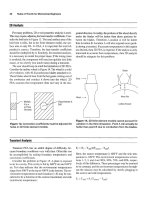
Figure
1.
Parametric design: single-shrouded total tem-
perature probe.
Figure
1
shows a general sensor configuration suited for
mach
0.3
to

0.8
with medium radiation effects.
This
design
is somewhat complicated to machine and would be con-
siderably more expensive than the sensor configuration
shown
in
Figure
2.
Differing fluid velocities and environ-
ment temperatures would require changing Figure
1
by
altering bleed hole diameters
(H),
adding other concentric
radiation shields, andor lengthening sensor
UD
ratios.
In
Figure
2,
the sensor hangs
in
a
pocket cut from a length
of
support
tube.

This
arrangement offers some radiation shield-
ing
(but decidedly inferior
to
that
in
Figure
1)
and some ve-
locity recovery. The placement
of
the sensor within the cut-
out will greatly influence the flow velocity over the sensor
and hence
its
recovery.
In
fact, depending on flow envi-
ronmental conditions (vibration, flow velocity, particles
within the flow, etc.) the sensor may
shift
within the pock-
et during use causing a change in reading
that
does not cor-
respond
to
a change
in

fluid conditions. The probe in Fig-
I7
Sensor Leadwires
Inshumentation
357
__*
Approximate
f<-
Relationships
A=
Clearance for sensor
B=
2A
C=
9A
D=
14A
E=
Defined
bv
structural needs
//
(typically
0
001
-
0.003
inches
loose)
*

'BI
C
11
ure
2,
therefore, is better suited for mach 0.1 to
0.4
in
areas with low radiation effects.
Figure
3
shows a compromise probe configuration in
terms
of cost and performance. It is designed for mach 0.1
to
0.4
with
medium
radiation effects. The perforations will
slow
the
flow somewhat less
than
the probe in Figure
1
and
will reduce radiation effects better than the probe
in
Fig-
ure

2.
This
contiguration does, however, have a sigmficant
advantage where flow direction can change. While the
probe in Figure
3
has stable recovery somewhat indepen-
dant of flow yaw angle, the probe
in
Figure
2
is very
sus-
ceptible
to
pitch angle variation and moderately suscepti-
ble
to
yaw variations. By comparison, the probe in Figure
1 is rather insensitive
to
yaw and
pitch
variations up
to
+30.
@A,-
\
-
Approximate

Relationships
(typically
4~)
F=
0.66E
G=
0.57E
I-'
View
AA
Fluid
1
~-
+D
Flow
G
.
~
-
Sensor
~
'74
+
@E
I
View
AA
Figure
2.
Parametric design: half-shielded

total
tem-
perature probe.
A=
Clearance for sensor
B=
Defined by structural needs
(typically
0.001
-
0.003
inches loose)
(typically
5.5A)
D=
2A*
E=
2A*
F=
9A
G=
1.5A
Sect
AA-AA
equally spaced,TYP
Figure
3.
Parametric design: multiflow direction
total
temperature probe.

358
Rules
of
Thumb
for
Mechanical Engineers
___
~ ~
_________~
Surface Temperature Measurement
Surface temperature measmment can be somewhat
eas-
ier than fluid temperature measurement due
to
fewer con-
figuration error sowes. Radiation effects can,
to
a large ex-
tent,
be
ignored,
as
a sensor placed
on
a surface
will
see the
same radiative flux
as
the surface beneath it would if the

sensor were not present. The only exception to
this
would
occur in high radiative flux environments where the sen-
sor has a significantly different emissivity than that of the
surface to
be
measured.
Error
sources,
then, for surface tem-
perature measurement
are
constrained
to
conduction and ve-
locity-induced effects.
Conduction errors occur when the sensor body contacts
an area
of
different temperature than that being measured.
The sensor then acts
as
an external heat transfer bridge be-
tween those
areas,
ultimately altering the temperature to
be
measured.
As

with fluid temperature measurement, a suf-
ficient sensor
L/D
ratio (between
8
and 15) will help en-
sure
that
conduction errors
are
minimized.
Velocity errors
are
present when the sensor body rests
above
the
surface
tobe
measuredand,
acting
lihe
ah
trans-
fers
heat between the surface and the
surrounding
fluid.
This
can occur in relatively low-flow velocities but is obvious-
ly worse with increasing fluid speed. Even at

low
speeds
the sensor can serve to trip the flow, disrupting the normal
boundary layer and increasing local heat transfer between
fluid and surface. Sensors that
are
of minimal cross-section
or are embedded into the surface of interest minimize ve-
locity errors. Embedding is preferred over surface mount-
ing because of the superior heat transfer
to
the sensor along
the increased surface area
of
the groove
(see
Figure
4).
Fill
(e.g., epoxy)
Flush
surface
Embedded Sensor
Large profile can disturb Minimal
flow
field
and
promote
convective
heat

transfer. (e.g., epoW area
Result:
poor
surface temperature reading
Joint
contact
w
Surface Mounted Sensor
Flgure
4.
Embedded versus surface mounting tech-
nique
for
surface temperature measurement.
Common Temperature Sensors
The most common temperature sensor is the
tkrmo-
couple
(T/C). In a T/C, two dissimilar metals are joined
to
form a junction, and
the
Rmainjng ends of the metal “leads”
are held at a reference (known) temperature where the
voltaic potential between those ends is measured. When
the
junction and reference temperatures are not equal, an elec-
tromotive force (emf) will be generated proportional to
the temperature difference. The single most important fact
to

remember about thermocouples is that emf will be gen-
erated only
in
areas
of the T/C where a temperature
gradi-
ent exists.
If
both the T/C junction and reference ends
are
kept at the same temperature TI, and the middle of
the
sen-
sor passes through a region of temperature
TZ,
the emf
generated by the junction end of the T/C
as
it passes from
TI to T2 will
be
directly canceled
by
the voltage generat-
ed
by the
lead
end of the T/C
as
it

passes
from
T2
to
TI.
Both
voltages will be equal in magnitude but opposite in sign,
with the net result being
no
output
(see
Example
1).
Fur-
ther explanation of thermocouple theory, including practi-
cal usage suggestions, can
be
found in Dr. Robert Moffat’s
The Gradient Approach
to
Thermocouple Circuitry
[2].
Thermocouples
are
inexpensive and relatively
accurate.
As
an example, chromel-alumel wire with
special
limits

of
error
has
a
0.4%
initial
accuracy
specification.
Tfi
can
be obtained
in
differing configuratons
from
as
small
as
sub-O.OO1-inch
diameter to larger
than
0.093-inch diameter and
can
be
used
from cryogenic
to
4,200”F.
However,
If
very high accuracy

is
required,
TICS can have drawbacks
in
that output voltage
drift
can
occur
with temperature cycles and sufficient
time
at
high
temperature, resulting in calibration
shifts.
’ho
other commonly used temperature sensors are re-
sistance temperature devices
(RTDs)
and thermistors, both
Instrumentation
359
Example
1
The Gradient Approach to Thermocouple Circuitry
Voltmeter
FFw;l
Alumel Alumel
500°F
750°F
32°F

70°F
Chrome1 Chrome1
Example
of
a Type
K
(Chromel-Alumel) thermocouple with its
junction
at
500°F
and reference temperature
of
32°F
where a splice
to the copper leadwires is made. In this example, the thermocouple
passes through a region of higher temperature
(750°F)
on
its
way to
the
32°F
reference.
The voltage
(E)
read
at the voltmeter can be represented
as
a
summation

of
the individual emfs
(E)
generated along each discrete
length of
wire.
The emf generated by each section is
a
function
of
the thermal
emf
coefficient of each material
and
the temperature
gradient through which it passes. Therefore:
32F
750°F
500°F
70°F
+J""'
750'F
EAL
+I,,,
Ecu
Rearranging and expanding, we see:
If the far left temperature zone was at
32°F
instead of
500"F,

all
equations would remain the same but the final form could be further
reduced to the following:
of which have sensing elements whose resistance changes
in
a
repeatable
way with temperature.
RTDs
are
usually con-
structed of platinum
wire,
while thermistors
are
of integrated
circuit chip design.
RTDs
can be used from
-436°F
to
+2,552"F,
while thermistors
are
usually relegated to the
-103°F to
+572"F
range. Each of these sensors can be
very accurate over its specified temperature range, but
both are sensitive to thermal and mechanical shock. Ther-

mistors do have an advantage in very high resistance
changes with temperature, however, those changes remain
linear over a relatively small temperature range.
One other surface temperature measurement technique
that
bears
mention is
pymmrerq:
which can
be
used to mea-
sure surface temperatures from +1,20O"F to
+2,00O"F.
When materials get hot they emit radiation
in
various
amounts at various wavelengths depending on temperature.
Pyrometers use this phenomenon by nonintnrsively mea-
suring
the emitted radiation at specific wavelengths
in
the
infrared region of the spectra given
off
by the surface
of
in-
terest and, provided the surface's emissivity is known, in-
ferring it's temperature. The equation
used

is
P=&d?
where
P
is the power per unit area in W/m2,
E
is the emis-
sivity of the part,
CJ
is the Stefan-Boltzmann constant
(5.67
*
1t8 W/(m2K4), and T is the temperature in
K.
Py-
rometers use band-pass filters to allow only specific
wavelength photons to reach silicon or InGaAs photodi-
odes, which then convert the incoming photons to elec-
trons yielding a current that is proportional to the tem-
perature of the part in question. These sensors are not
influenced by the above-mentioned physical error sources
(because they are nonintrusive) but can be greatly
af-
fected by incorrect emissivity assessments, changes in
emissivity over time, and reflected radiation from other
sources such as hot neighboring parts or flames.
Theory
based
on
Moffat

[21.
PRESSURE MEASUREMENT
Pressure measurement can
be
divided
into
two
axas:
total
pressure and static (or cavity) pressure. In most cases it
won't
be
practical to place
a
pressure transducer directly
into
the fluid in question or even mount it directly
to
the flow-
containing wall because
of
the vibration, space, and tem-
perature
limitations of the transducer. Instead, it is common
practice to mount the open end of a tube at the sensing lo-
cation and route the other end of the
tube
to a separately
380
Rules

of
Thumb
for
Mechanical Engineers
mounted transducer. Due to this consideration, the re-
naainder of this section concentrates
on
tube mounting de-
sign considerations. Pressure transducers can be chosen
as
stock vendor supplies that simply meet the requirements in
terms of accuracy, frequency response, pressure range,
over-range, sensitivity, temperature
shift,
nonlinearity and
hysterisis, resonant frequency, and zero offset, and will
not be further discussed here.
Total
Pressure
Measurement
As with temperature, fluid pressure readings can
be
sta-
tic or total. Static pressure
(P,)
is the pressure that would
be
encountered if one could travel along with the fluid at
its exact velocity, and total pressure
(Pt)

is that pressure
found when flow is stopped, trading
its
kinetic energy for
pressure
rise
above
P,.
P, and
Pt
are related by the
equation:
PJP,
=
[
1
+
H
(y
-
1)M2]v(Y-
I)
where
y
is the ratio of specific heats (c#$ and equals 1.4
for air at
15°C.
M
is the mach number. See Table
1

for tab-
ular
form of
this equation.
The most common method of measuring
Pt
is to place a
small tube (pressure probe) within the fluid at the point of
interest and use the tube to guide pressure pulses back
to
an externally mounted pressure transducer. Error sources
for this arrangement include inherent errors within the
pressure transducer, response time errors for nonconstant
flow conditions, and errors based on incorrect tube align-
ment into the flow and/or configuration.
In order
to
minimize response time lags, the pressure
transducer should be mounted as close as practical to the
point of measurement. Also, the tube's inner cross-sec-
tional area should not be significantly smaller than the
outer diameter
ratio
of
0.2
and a
15"
chamfer; and (d) is a
cylinder in cross flow with a capped end and a
small

hole
in its wall. As shown in Figure
0.2,
each of these arrange-
ments has a differing ability to accept angled flow and
still transfer Pt accurately
to
its transducer.
While the head modifications compensate for improper
flow angle, another
error
can
occw
if
pressure
gradients exist
within the flow. In the subsonic flow regime discussed
here, the flow
can
sense and respond to the presence of the
pressure probe within
it.
As a result, the flow will turn and
shift toward the lower pressure area when presented
with
the blockage of the pressure probe. By ensuring that the
length
of
tube along the flow direction is at least three
times the width of the body to which the tube is mounted

(with the body perpendicular
to
the flow direction),
this
ef-
fect can be minimized (see Figure
6).
Subsonic
t
U
(a)
Impact
(b) Shielded
ire Tube
Containing
T hm
PI
(c) Chamfered (d) Cylinder
Tube in
cross
flow
pressure
transducer's
referencivolume, located immediately
in
front of its measuring diaphragm. Additionally, increases
in the tube's cross-sectional area between the sensing point
and
the
transducer

will
slow response
time.
Finally,
the tub-
ing should
be
seamless when possible and have minimal
bends. All necessary bends should
be
constructed with a
minimum inner radius of 1.5 times the tube's outer diam-
eter (for annealed metallic tubing).
For the tube to correctly recover the full Pt, it is critical
that
the
sensor
(tube)
face directly into the flow.
Often
it may
not
be
possible to know flow direction accurately, or the
flow angle is
known
to change during operation. In these
cases, modifications to the tube sensing end must be used
to
correct for flow angle discrepancies.

In
Figure
5,
four tube
end arrangements are shown: (a) shows a sharp-edged im-
pact tube; (b) adds a shield; (c) is a tube with an inner to
IWBLE.
e.
CES
Figure
5.
TU
pressure
probe,
tube
sensiw
end
-,
and
emr
with
respect
to
flow
angle
[l].
(Cou&sy
of
In-
sfnrment

SoCiety
of
America.
Reprintecl
bypmjssion~)
Instrumentation
361
Pressure Gradient
8o
r
yEPres; Displacement
of
I
I
I
I
I
1
1
2
3456
0'
Ratio
of
Length
of
Sensing
Element to Diameter
of
Support

(b)
Figure
6.
Total pressure probe
errors
of
pressure gradient displacement due to sensing tube length
[l].
(Courtesy
of instrument Society
of
America. Reprinted
by
permission.)
StaticlCavity
Pressure
Measurement
While it is difficult
to
measure static pressure
(PJ
ac-
curately within
the
flow
(as
any intrusive sensor
will
recover
a significant portion of

Pt
-
P,,
and the
P,
probes that have
been designed
are
sensitive to flow angle), it is relatively
easy to measure
P,
using a hole in the wall that contains
the
flow. Either the pressure transducer can be
directly
mount-
ed
to the wall or, more
unnmonly,
a tube
will
be
placed flush
with
the
inner wall at the sensing end
with
a pressure
trans-
ducer connected to the opposite end.

Error sources in obtaining accurate static pressure mea-
surements fall into
the
same categories
as
those
of
total
pres-
sure,
with
inherent errors caused by the pressure transduc-
er, response-time errors for non-constant flow conditions,
and
errors
based
on
incorrect tube alignment at the wall.
Re
sponse-time errors
are
very similar to those found in
total
pressure measurement systems.
To
reduce response-time er-
rors,
keep all tubing lengths
as
short as possible and

min-
imize
bending. For all necessary bends, keep a minimum
inner radius of 1.5 times the tube outer diameter (for an-
nealed, seamless, metallic tubing).
Finally,
minimize
all in-
creases
in
the tube cross-sectional
area
between the sens-
ing point and
the
sensor.
Static pressure errors related to configuration
are
some-
what more complex.
As
shown in
Figure
7,
the size of the
static pressure port diameter (tube inner diameter in most
-
1.2
ae
-

v
e
Water
Hole
Size
(Inches)
Figure
7.
Errors
in static
pressure
reading
as
a function
of
hole size
for
air and water
[4].
(Reprinted
by
permis-
sion
of
ASME.)
cases) can
produce
errors
and
must

be
balanced
against
prac-
tical machining considerations and flow realities. While
a
0.010-inch inner tube diameter
may
provide
a
very accu-
rate reading, it may not be practical to obtain tubing of that
size
or
to
machine
the
required
holes.
In
addition,
if
the
flow
field consists of highly viscous oil or air with high partic-
362
Rules
of
Thumb
for

Mechanical Engineers
ulate count (soot, rust, etc.) then a 0.010-inch diameter
orifice would impede pressure pulse propagation and/or
would plug completely.
Not only
is
static pressure port diameter a considera-
tion, but changes in that port diameter along its length close
to the opening to the flow field can also
be
a source of error.
It is a good rule of thumb not to allow changes in the stat-
ic pressure port diameter to occur within a length of 2.5 times
the static pressure port diameter itself. For example, if a
0.020-inch diameter hole is added to a pipe for the purpose
of measuring static pressure in the pipe, then the 0.020
hole should remain that size, with no interruptions or steps
for at least
0.050
inches away from the opening to the pipe.
A
length of 3.0 to
5.0
times the hole diameter is preferred
where practical. See
ASME Power
Test
Codes, Supplement
on Instruments and Apparatus:
Part

5,
Measurement of
Quantity of Materials, Chapter
4:
Flow Measurement, copy-
right 1959.
A
final effect to be considered concerns that of orifice
edge and hole angle with respect to the flow path (see Fig-
ure
8).
It is best to keep the hole perpendicular to the flow
and retain sharp edges. Failure to remove burrs created dur-
ing hole machining can give negative errors of 1520% of
dynamic head, while failure to completely remove the
burrs (e.g., burr area cannot be detected by touch but is vis-
ibly brighter than surrounding area) can give negative er-
rors up to 2% of the dynamic head. For these reasons, the
note to “remove burrs but leave sharp edges’’ should always
be used when calling out the machining of static pressure
ports holes on a drawing. See “Influence of Orifice Geom-
etry on Static Pressure Measurement,”
R.
E.
Rayle, ASME
Paper Number 59-A-234.
4bF
j
FF“.‘”
+at%

-04
n
Figure
8.
Effect of orifice edge form on static pressure
measurements (variation in percent of dynamic head)
[4].
(Reprinted
by
permission
of ASME.)
It
is
often necessary to discern the stress within a com-
ponent of interest. As there are no practical ways to obtain
stress information directly, it is customary to measure strain
(E)
and, using the material’s known modulus of elasticity
(E),
calculate the stress
(0)
via the equation:
O=E&
Strain is simply the change in length
(AL)
of a material di-
vided by the length over which that change is measured
(gauge length,
L).
As

an example,
if
the original length be-
tween two known points on a surface of interest is
l
.OOOO
inches, and the length measured under loading is found to
be 1.0001 inches, then the change in length is 0.0001 and
the gauge length is 1
.OOOO.
The strain is therefore:
ALL,
=
0.0001/1.0000
=
0.0001 strain
As strain numbers are usually very small, it is customary
to use the units of microstrain
(p),
which are
lo6
times nor-
mal strain values. The above example would be read as
The following sections highlight the electrical resis-
tance strain gauge and its common data acquisition system.
Additionally, some effort is made to discuss compensation
techniques to provide a customer-oriented output useful in
a variety of conditions.
loop.
Instrumentation

363
The Electrical Resistance
Strain
Gauge
The most common strain measurement transducer is the
electrical resistance strain gauge.
In
this sensor, an electrical
conductor is bonded to the surface of interest. As the sur-
face
is
strained, the conductor will become somewhat
longer (assuming the strain field is aligned longitudinally
with the conductor) and the cross-sectional area of the
conductor will decrease. Additionally,
the
specific resistivity
of the material may change. The summation of these three
effects will result in a net change in resistance of the con-
ductor, which can be measured and used to infer the strain
in the surface. The relationship that ties this change in re-
sistance to strain level is:
GF
=
[AR/R]k
where GF is the gauge factor of the specific gauge,
dR
is
the change in gauge resistance,
R

is the initial gauge re-
sistance, and
E
is the strain in incheshnch (not
p~).
Electrical resistance strain gauges can be purchased in
a variety of sizes as fine wire grids (e.g., 0.001-inch di-
ameter) but are more commonly available as thin film foil
patterns. These foil gauges offer high repeatability,
a
wide
variety of grid
sizes
and orientations, and a multitude of sol-
der tab arrangements. Multiple gauge alloys are available,
each with characteristics suited for a trade-off between fa-
tigue life, stability, temperature range, etc. The gauges can
also be purchased with self temperature compensation
(STC) which serves to match the general coefficient of ther-
mal
expansion of the part to which the gauge will be bond-
ed, thereby reducing the “apparent strain” (see the Full
Wheatstone Compensation Techniques section).
In
addition
to multiple alloys, there
are
multiple gauge backing mate-
rials from which to choose. The gauge backing serves to
both electrically isolate the gauge from ground and to

transfer the strain to the alloy grid. Finally, gauges can be
purchased with the grid exposed or fully encapsulated for
grid protection. Once these choices
are
made, it is still
necessary to pick
the
proper cement, leadwire, and solder.
As
was stressed in the introduction, relying on the tech-
nical expertise of a competent vendor is critical
in
obtain-
ing usable results with
an
unfamiliar
sensor system.
This
is
paaicularily true with strain gauge application. There are
so
many variables, choices, and error sources that, without
solid technical counseling, the chances for obtaining poor
data
are relatively high. It is beyond the scope of
this
chap-
ter to go through the finer points
of
gauge application, es-

pecially with the excellent vendor literature available. How-
ever, some common failure points in gauge application
include the areas
of improper cleanliness of the part (and the
hands
of
the
gauge application technician), improper part
sur-
face
finish, and poor solder
joints
or incomplete flux removal.
Keeping the gauge area on the part clean and free of
ox-
ides is critical to obtaining a good gauge bond. Once the area
is clean, install the gauge in
a
timely manner so as not to
allow the area to pick up dirt. Perform the cleaning and
gauge application in a draft-free, air-conditioned area when
possible. This will provide the air with some humidity
control and filtering. Not only does the part need to be
cleaned, but it is also good practice to have the technician
wash his hands prior to beginning each gauge application.
This will reduce contamination of the gauge area with
dirt,
oil, and salts from the skin.
Additionally, if the part surface has a rough surface fin-
ish in the gauge area, an inconsistent adhesive line thick-

ness can exist across the gauge.
This
can yield poor strain
transfer to the gauge, especially
if
the part is subject to tem-
perature excursions where thermal expansion mismatch
between the part and cement can cause unwanted grid de-
flection. Problems can also exist, however, if the part has
a surface finish that is smooth like glass.
In
this case, in-
sufficient tooth may exist to obtain maximum cement ad-
hesion, resulting in gauge slippage at high strains or under
high cycle fatigue. Again, follow the manufacturer’s rec-
ommendations (usually,
60
pin, rms is the recommended
surface finish).
Finally, it is common practice to use some flux to aid in
soldering the lead wires to the strain gauge tabs to assure
proper solder wetting. However, flux residue
that
is not com-
pletely removed can serve to corrode the metals and even-
tually cause shorts to ground. What is insidious about this
failure mode is how slowly it works. Flux residue can go
unnoticed as the gauge is checked, covered with protective
coatings, and delivered to
test.

Then, during the test phase
when critical data are being taken, the gauge can develop
intermittent signal spikes and drop-outs, eventually re-
sulting in low resistance
to
ground.
364
Rules
of
Thumb
for
Mechanical Engineers
V
G;
07;
-E
-V€
Electrical Resistance Strain Gauge
Data
Acquisition
Single active gage in uniaxial
tension or compression.
Two
active gages with equal
and oppositestrains- typical
of
bending-beam arrangement.
Four active gages in uniaxial
stressfield-twoaligned with
maximum principal strain, two

"Poisson" gages (column).
Four active gages with pairs
subjected
to
equal and oppo-
site strains (beam in bending
or
shaft
in torsion).
One common method for measuring the gauge resis-
tance changes caused by strains is the Wheatstone Bridge
completion circuit. This circuit can have one, two, or four
active legs corresponding to single-gauge configuration
(Le.,
!4
bridge), two-gauge configuration (i.e.,
H
bridge), and
four-gauge configuration (full bridge). Figure
9
shows
!4,
E,
and full bridge arrangements together with their repre-
sentative output equations. Let
us
examine the full bridge
configuration.
Description
B*dge'stra'n

Arrangement
I
Output
VOIV
(mVN)
a1
Gaga
Factor.
F.
when
4
+
2FE
x
IO+
Figure
9.
Full, one-half, and one-quarter active bridge
arrangements with output voltage equations.
(Courtesy
of
Measuremenfs
Group,
Inc.,
Raleigh,
NC.)
In a simple, uniform cantilever
beam
with a single load
on the free end deflecting the beam downward, the top

surface of the
beam
is
in
tension and
the
bottom
of
the
beam
is in compression (Figure
10).
As
shown,
the
neutral
axis
of the beam is located along the beam's centerhe which
implies that the strain on the beam's top
surface
is equal in
magnitude to the strain on the beam's bottom surface.
To
determine the strain in the beam, gauges
#1
and
#2
should
be
placed on the top surface of the

beam
and gauges
#3
and
#4
should
be
placed
on
the bottom.
All
four of the gauges
should
be
oriented longitudinally along the
beam
at
the
same
distance
from
the fixed end. The gauges should then be
wired as shown
in
Figure
11.
From Figure
10
we can
see

that the calculated strain
along either surface's outer fibers at the
strain
gauge loca-
Top
View
Neural
I
Section
AA-AA Axis
Scale
2x
E1
where
P
=
25
Ibs
E
=
6.25 inches
L
=
7.00
inches
b
=
1.00
inch
h

=
0.25 inches
c
=
0.125 inchzs
E
=
0.0005
idin
=
500
J~E
Figure
IO.
Simple uniform cantilever beam with full
bridge
to measure bending.
tion equals
500~.
Each single
350
i2
gauge (with a gauge
factor of
2.
l),
placed longitudinally in
this
location, would
see a resistance change

of:
AR
=
R(E)
GF
AR
=
(350)(0.OOO5)(2.1)
=
0.3675
O~S
Therefore, the two gauges in compression each read
349.6325
under load while the
two
gauges
in
tension each
read
350.3675
under load. With
an
input voltage
of
5.0
volts,
the output voltage equals
5.25
mV (see Figure
11).

To
have
the Wheatstone Bridge perform properly, the
bridge
must
be
balanced
That
is, each leg must have the
same
resistance, otherwise, a voltage output will
be
present under
zero
strain
conditions. Unbalanced situations
occur
due
to
in-
herent resistance differences between gauges
in
the bridge
coupled with resistance differences due to different length
in-
ternal bridge wires. Balancing
can
be
performed external to
the bridge with the use of many readout devices; however,

it
can
also
be handled within the bridge circuitry, simplrfy-
ing
futm
data
acquisition concerns. Special resistors
can
be
bonded within the circuit and then trimmed to leave the
bridge output at just a few microstrain under zero load.
Instrumentation
365
I-
+
Power
Gauge
#4
Gauge
#1
-
v2
Signal
A
+
Signal
v,
x-
Power

-
-
R
3
L‘,
For
350
0
gauges,
GF
=
2.
1,
Strain in each element
=
500
p&
and V,,
=
5.0V
Then
VI
=
2.502625V and
V2
=
2.497375V and
VI
-
V2

=
0.00525V
=
5.25
mV
VI
=-
R,
+
R1
V?
-
RrVLn
RZ+R,
Figure
I
I.
Wheatstone wiring diagram for beam in
bending; calculations for beam in Figure
12.
Full
Wheatstone Bridge Compensation Techniques
If the
beam
in Figure 10 is to
be
used at elevated (or re-
duced) temperatures, further compensation for “apparent
strain”
(G)

and “modulus” may be used to optimize the
data
for the customer. Apparent
strain
compensation helps ac-
count for
strain
output resulting from no-load temperature ex-
cursions. These extraneous readings are caused by (1) tem-
perakm coefficient of resistance (TCR) changes in the gauges
and wiring of the bridge and
(2)
differences in thermal ex-
pansion between the component being instrumented and the
gauge itself. Modulus compensation attempts to account for
additional extraneous
strain
output at temperature caused by
both
changes
in
the
strain
sensor’s gauge factor (GF) with tem-
perature and changes in component modulus of elasticity
(E),
allowing the data to represent only the strain due to
load.
This
last compensation allows the design engineer to use

the
data
without having
to
know
specific
time-temperam
his-
tory
to input varying E and GF values to get
true
stress.
As
further clarification of
this
compensation issue, it may
be viewed as follows: If the part can be taken through a
temperature excursion in a no-load condition and the
gauge output remains essentially zero, then the gauge re-
quires no (further)
compensation. If the part can be
taken through a temperature excursion under load and the
gauge output represents accurately the load conditions in-
dependent of temperature, then the sensor requires no
(further) modulus compensation.
Apparent strain can be corrected by (1) using the correct
STC (self temperature compensating) gauges,
(2)
com-
pensating with the addition of special wire segments or

trim-
mable bondable foil patterns within the bridge itself, or
(3)
both. The compensating wire or foil pattern used in
(2)
and
(3)
is chosen such that its TCR will serve to balance the un-
desirable TCR changes in the bridge wiring and gauges.
This
compensation step is required if the
STC
gauges don’t ac-
curately match the part’s coefficient
of thermal expansion,
or if higher accuracy is required than offered by the gen-
eralized STC gauges.
Compensation by addition of wire or foil resistors can be
accomplished by starting with a balanced bridge bonded to
the component of interest. Attach the bridge to a quality
strain output measurement device (it should
read
very close
to
zero
microstrain if balanced well) and place temperature
sensors on the component in various locations. Place the
component in
an
oven,

or
other environmental chamber, that
can duplicate the expected operating temperature. Subject
the component to
a
temperature that will stabilize the
gauge/epoxy system (preferably
25” to
50°F
above the ex-
pected operating temperaturej. The part should remain at
this temperature until the strain output varies by less than
2
microstrain per hour for two consecutive hours. Return
the component to room temperature. When the part is
cooled and isothermal,
record
the strain output. Finally, sub-
ject the component to its operating temperature and record
the strain output change from the last reading. This is the
uncompensated
sapp.
At
this
point resistors of appropriate TCR need to be
added to the correct bridge legs to balance the uncompen-
sated
capp.
It
is known that

AR
=
R(E) GF
Rewriting and expanding
this
equation, we see that:
where
Gq
is the additional compensating resistance to
be
added,
R
is the bridge resistance, AT is the change in tem-
perature from room temperature to operating temperature,
and
TCR
is the temperature coefficient of resistance
of
KOmp
(e.g., TCRBal,,
=
0.0025”F’).
Returning to Figure
11,
if the
sapp
reading showed that
V2
had a higher poten-
tial

than
VI,
then we can infer that resistance should be
added to the leg containing either
&
or
R3.
After the resistor
366
Rules
of
Thumb
for
Mechanical Engineers
has been correctly inserted, it is good practice to recheck
the at temperature.
Unk apparent
strain
compensation, which involves plac-
ing a special resistor within the bridge circuit itself, modulus
compensation involves placing two resistors, one in each of
the power legs leading to the bridge. These resistors should
be
placed as close to the bridge
as
possible so as to
be
with-
in the same thermal environment, thereby responding to tem-
perature changes with resistance changes that adjust the

bridge input voltage. Although it is best to test the bridge out-
put at temperature under known load to calculate modulus
cornpensdon,
it
is
often
not
practical.
Therefore, the following
formula may be used to estimate the resistances
required:
R(GF2E1- GFlE2)
GFlb
+
(GF1
X
El
X
TCR
(T2
-
Ti))
-
GFzEl
R,
=
where
bC
=
the resistance to

be
split equally between the
positive power and negative power legs
(n),
R
=
the bridge
resistance
(a),
TI
=
room temperature
(“F),
T2 =bridge
op-
erating temperature
(OF),
El
=
the component material
modulus of elasticity at TI (psi),
E2
=
the component
ma-
terial modulus of elasticity at
T2,
GF1
=
the gauge factor of

the bridge gauges at
TI, GF2
=
the gauge factor of the
bridge gauges at T2, and
TCR
=
the temperature coefficient
of resistance of the compensating resistors
(“I?).
LIQUID LEVEL AND FLUID FLOW MEASUREMENT
The measurement of liquid level and fluid
flow
rate is re-
quired in virtually all aspects
of industrial process control
and power generationlconversion. Due
to
the widespread
need for these measurements and the similar nature of
vir-
tually
all
liquid storage and fluid delivery (piping) sys-
tems, common sensor solutions are readily available from
a well-established vendor base. These sensor packages can
meet a wide variety of price and accuracy requirements and
can be tailored to almost any liquid, regardless of proper-
ties.
In

addition, much work has been done by the techni-
cal societies to standardize on measurement methodologies
and practices.
As
a result of these readily available systems and stan-
dards,
this
chapter
will
not
stress
fundamental theory or prac-
tices necessary to custom-design specialized sensor pack-
ages. Instead, it will simply outline some of the more
common level and flow systems available, detailing cost,
ac-
curacy, and environmental considerations where applicable
and suggesting general rules to use
in
making a selection.
The sensor vendors will be familiar with the vast majority
of level and flow problems and
be
able
to recommend
“off-
the-shelf” solutions. Should highly specialized cases
occur,
additional
information

on
the
design
and
development of
cus-
tom systems can be obtained
from
the reference literature.
~ ~~
liquid level Measurement
Level
sensors
relay information regarding the interface
between a liquid and
a
gas (often air) or the interface be-
tween two liquids of differing specific gravities. The sen-
sors can be point-specific or continuous-reading. Point-
specific level sensors trip a switch when
the
liquid interface
reaches a set point. These switches might activate alarms,
open valves,
turn
on
pumps, etc. Continuous-reading level
sensors relay values corresponding to interface position
within
an

operating range. The information from continu-
ous-reading sensors may be used as diagnostic data or as
input to a control system.
Level sensors rely on measuring buoyant forces, pres-
sures, timing of ultrasonic pulses, etc., to infer the location
of the interface in question. These sensors range from sim-
ple floats that move with the interface (as used in a sump
pump), to more complex sensors measuring capacitance
fluctuations as the fluid changes height between conduc-
tive “plates.”
In
this
chapter we will quickly compare the
following most common level sensors: float, displacer,
delta-pressure systems, capacitance, and ultrasonic.
The simpleflout
sensor
relies
on
the buoyant force of the
liquid in question to maintain
the
float at a specific relation
to the liquid interface. In Figure
12
(a)
a
float switch
is
at-

tached to a motion transducer providing a continuous
read-
ing system. In the sump pump reference above, the float
is
attached to a switch, creating
a
point-specific system.
These switches can be designed
so
that a permanent mag-
net on the end of the float rod actuates a hermetically
sealed reed switch, making a very rugged system.
Float
sen-
sors are generally economical, rugged, repeatable, and
us-
Instrumentation
367
-00
pg+
CI
P
la
Figure
12.
Various liquid level measurement meters
[9].
(Reprinted
by
permission

of
McGraw-Hill
Book
Co.)
able with a wide variety of fluids. They are relatively in-
sensitive to shock and vibration. Some particularily inex-
pensive float switches, however, may fail after a time in ser-
vice due to their economical construction. If very low-cost
float switches are chosen, it may be prudent to install two
independent sensor systems to minimize risks.
The
displucer
sensol;
Figure
12
(b), is related to the
simple float in that it relies on the fluid’s buoyant force and
is usable with many fluids. Unlike the float, however, it does
not follow the liquid interface. Instead, the changing in-
terface alters the buoyant force on the quasi-stationary dis-
placer, and that change in force is read on an attached
force transducer. The displacer
’s
construction allows for ac-
curate resolution of small level changes, but its force trans-
ducer can make it more sensitive to shock and vibration.
Delta-pressure
systems,
Figures 12 (c) and (d), use the
hydrostatic pressure of the liquid to infer the interface lo-

cation. The pressure force of the column of fluid is a func-
tion of the liquid level times the fluid’s specific weight. With
the open container situation, the pressure gauge should be
chosen to measure “gauge pressure.” If an absolute pres-
sure gauge were chosen, it would measure the weight of both
the
liquid and the column of air above it (barometric pres-
sure); changes in the barometer would adversely affect the
repeatability of the system.
The pressure vessel situation requires the use
of
a dif-
ferential pressure sensor to compensate for the column of
vapor over the liquid interface. Both
of
these techniques can
be used in limited slurries and corrosives if proper pre-
cautions such as liquid seals, water purge, or air purge are
used to isolate the pressure meter from the process.
Capacitance-based sensors
use a probe and the wall
of
the vessel as two plates of a capacitor with the liquid medi-
um between as a dielectric.
As
the liquid level changes, the
effective capacitance between the “plates” is altered in a re-
peatable manner. For fluids that are nonconducting (di-
electric constant
<

4) the probe can be inserted directly into
the liquid-see Figure 14 (e). For conductive fluids, the
probe must be insulated to keep the liquid from short-cir-
cuiting
the
system-see Figure
12
(f).
Should the vessel be
nonconducting, a second probe can be inserted into the fluid
to act as the second capacitor plate.
Capacitance level sensors can be used with many com-
mon liquids (including many liquid metals and corrosives)
and granular solids. They can be operated through a wide
temperature and pressure range. In the case where fluid tur-
bulence is possible, the probe(s) must be designed
so
as not
to move. Even small changes in the probe’s position will
alter the effective distance between capacitor plates and will
appear to the sensor as a level change!
Ultrasonic level sensors
transmit and then read high-fre-
quency pressure pulses to infer interface levels. In the case
of noncontacting sensors, Figure
13
(a), the ultrasonic
beam strikes the fluid surface and the echo is detected by
the sensor, creating a continuous reading sensor.
As

in
sonar, the timing of the signals indicates the distance be-
tween the probe and the “surface” that created the echo.
Some of these sensors utilize additional software that cre-
ates a running average of the distance signals being received.
New signals are compared to this running average and to
new signals; in this way, spurious signals and noise can be
Non-Contact
Sensor
Contact
Sensor
(4
(b)
Figure
13.
Ultrasonic liquid level measurement sensors.
368
Rules
of
Thumb
for
Mechanical Engineers
identified and rejected.
As
noncontacting sensors, these ul-
trasonic sensors
are
of great value when highly corrosive
liquids and/or adverse environmental conditions exist.
Their accuracy and repeatability, however, drop as a func-

tion of the distance between probe and the liquid interface.
Contact ultrasonic sensors, Figure 13 (b), contain a gap
between the point at which the high-frequency pulse is
generated and a point farther along the probe where that
pulse is detected. The sensor is positioned
so
that the gap
is located in a known point
in
the fluid vessel. When the liq-
uid rises to the point where it fills this gap, the signal eas-
ily propagates from the pulse generator to the detector.
When the liquid level falls, the si-4
is
attend,
resulting
in a relay switching. In order to compensate for some sur-
face turbulence and agitation, delay logic is built into the
probe circuitry
so
the relay will not switch immediately.
These contact sensors are usable with most fluids,
however, highly aerated fluids can cause the signal to
remain attenuated even when the fluid is filling the gap.
Additionally, highly viscous liquids may cause errors
should the fluid remain in the gap after the liquid inter-
face level has dropped.
Fluid
Flow
Measurement

There are an exhaustive number of flow meters available
on the market to
fit
virtually any flow measurement need.
The most common flow meters can be divided into the
four main areas of differential pressure, positive displace-
ment, velocity, and
mass.
Differential flow meters include
orifice, target, venturi, flow nozzle, pitot tube, elbow, and
variable-area meters. Piston, oval gear, and rotary vane
meters
are
types of positive displacement flow meters. Ve-
locity meters include turbine, vortex, electromagnetic, and
ultrasonic variations. Finally, Coriolis meters measure the
mass rate of flow directly and
are
the most common of the
mass meters.
The most common flow meter in use today is the orifice
meter, primarily because of its wide pressure and temper-
ature operating range, low cost, and reasonable accuracy.
In Table
2,
a
comparison of
all
of the above meters is out-
lined, stressing summary characteristics. This table can be

used in making an initial selection of the few meters that
should be pursued in greater detail for the required appli-
cation. Should an orifice meter, venturi, or flow meter be
selected,
ASME
has some excellent literature available to
aid in the selection and design (e.g.,
Fluid Meters,
6th ed.,
ASME,
1971, and
ASME Power Test Codes, Supplement on
Instruments and Apparatus:
Part
5,
Measurement of Quan-
tity of Materials, Chapter
4:
Flow Measurement, copy-
right 1959). Additional information on the selection and
design
of
custom systems can be obtained from the refer-
ence literature.
Orifices are
thin, flat plates of metal placed between
flanges of the flow-carrying pipe
so
as to block flow. These
plates have specific configuration openings machined into

them that allow the flow to pass through. Static pressure taps
on each side of the plate allow the measurement of the dif-
ferential
pressure
caused by the flow obstruction. By know-
ing the size and configuration of
the
opening in the orifice
plate and the
two
pressure readings,
the
flow
rate
can
be
de-
duced.
The
orifice
is
especially subject to errors due to wear
and abrasion.
Target meters
measure the force imparted on a target
placed in the flow. The force is the upstream pressure
minus the downstream pressure integrated over the area of
the target, and is therefore directly related to the flow rate.
Venturi meters
are

a section of piping that has
a
grad-
ually inward-sloping entrance section (approximately
21
O
included angle), a straight section
of
reduced diameter,
and a gradually sloping exit section (approximately
8”
in-
cluded angle). Static pressure measurements taken prior to
the entrance section and
at
the reduced diameter “throat”
allow calculation
of
the flow
rate.
The venturi offers
redud
abrasion characteristics when compared to the orifice
meter.
Flow
nozzles
are
literally nozzles inserted concentrically
into the flow path to gradually reduce the pipe area and then
dump the flow back to the original pipe diameter. Flow noz-

zles possess the same general accuracy and resistance to
abrasion advantages of the venturi while offering a short-
er installed length and
a
cheaper price. These nozzles,
however,
are
more costly than orifices, have pressure
re-
covery performance between
that
of the orifice and venturi,
and are somewhat difficult to install.
Pitot
tubes
use total and static pressure readings at a
sin-
gle flow stream, via an inserted probe,
to
determine flow
velocity and flow rates.
As
stated in the Static
Pressure
Mea-
surement section,
it
is difficult to measure
P,
in a flow field

due to flow angle sensitivity
of
the inserted probes.
If
the
flow field is very well established, pitot tubes that measure
total pressure at their
tips
and static pressure along the
Table
2
Comparison
of
Flow
Meters
Flow
Meter
Orifice,
Flow nozzle
square-edged
Ventud
QAS
LIQUIDS
temperature pressure including Reynolds Plpe upstream Pressure
Relative
clean dlrty clean dirty viscous corrosive slurry
"F
wig1 transmitter number size,
in.
pipe, diam.

loss
Range
cost
to
1,000
(transmitter
to
0 0
0 0 0 0.
X
X
250)
to
6000
*l-2%URV*
RD
>
1,000
>
1.5 10-30
medium
41
low
I
X
X
rld%URV
RD>100
>.5-4
10-30

medium
41
medium
+1-2%
URV
RD
>
75,000
>
2 5-20
low
41
medium
OX*
X X
X
X
0x0
X
X X
+1-2%URV
Ro
>
10,000
>
2 10-30
medium
41
medium
I

0
Mass
flow
disdacement
0
X
I
I
I
+3S%URV
I
>3
I
20-30
I
very~ow
1
31
0x0
X
X
X
I
+!%lO%URV IR1,>10,000
I
>2
I
30
I
verylow

I
31
nolimit
I
low
low
I
Turbine
I*
X
I
500
I
S3000
0 0
0
Ultrasonic
Ultrasonic
(time of flight)
(Doppler)
Variable area
5
Electromaanetlc
I
360
I
4500
1
d.5%
of

rat0
I
nolimit
I
.l-72
I
none
I
401
I
hlgh
*x
)x
0
0
X
X
<
570 42000
gas:
250
0
51
400
X
liquid
600
gas:
21
%

URV
liquid
d.5%
of
rate
gas:
+0.5%
of
rate
Pipe
ratlng
pipe
rating
glass:
350
metal:
720
51 500
18,000
cst
42
none hlgh
101
medium
+oA%
of
rate
I
no limit
I

I
none
I
low
I
101
I
hiah
liquid:
+1%
or
rate
e1 %
URV to
+5%
of
rate
+5%
of
URV
+0.5%
of
rate
to
rl
YO
URV
+0.5-1.5%
of
rate

12-1 5
cSt
25-24
+lo
high
201
high
no limit
>.5
5-30
none
201
high
no limit
>.5
5-30
none
101
hlgh
to highly
viscous fluid
13
none medium
101
low
~10,000
5-18 1b20
medium
101
hlgh

0
X
0
0
X
0
0
I
I I
I
I
Designed for this application
x
Normally applicable
(no
symbol)
Not designed
for
this application
WRK
Upper
range
value
of
the
flow
(fomedy
full-scale flow
rate)
Sources:

Adapted
from
Milkp],
by
mission
of
McGraw-Hill
Book
Co.,
and
Plant Engineehg,
Now
21,
1984,
copyright
@
Cahners Publishing
Co.,
by permission.
500
250
0
X
0
X X
glass:
1400
metal:
51
000

1750
370
Rules
of
Thumb
for
Mechanical Engineers
probe bodies can be used. When flow profiles change with-
in the pipe, a single-point pitot tube can show errors due to
both improper
P,
values and the fact that the single-point
measurement no longer represents the true average veloc-
ity. Averaging pitot tubes, which sample multiple loca-
tions in the flow, are often used
as
a more accurate measure
of the flow field velocity.
Elbow meters use the principle that fluid flowing along
the outer path of a turn will exert a centrifugal force that
is proportional to fluid velocity. Static pressure taps are
placed in the inner radius and outer radius of the elbow.
Variable-area meters have a float, suspended in a ver-
tical section of slightly diverging “pipe” diameter. The di-
verging flow section allows flow to pass by the float on the
sides. The float’s position in that section
is
a function of the
flow rate and always seeks the equilibrium point where the
differential pressure on the float is balanced by

the
force of
gravity on the float.
Positive
displacement
flow
meters separate the flow into
established sections of known volume as the flow passes
through the meter. By counting the throughput frequency
of those sections, the flow rate is deduced.
Turbine meters utilize a free-wheeling rotor placed
within the flow stream.
As
flow rate increases, the rotor
speed increases. By measuring the frequency of the rotor,
the flow rate can be calculated. Potential error sources for
turbine meters include calibration shifts due to blade wear,
bearing wear (and its associated increase in friction), and
overspeed when packets of vapor enter the
meter.
Vortex meters
utilize the approximately sinusoidal
pres-
sure (and velocity) changes that are caused by moving
vortices shed by a bluff-body placed
in
the flow
stream.
The
frequency of the vortex shedding is a function of the fluid

velocity and, therefore,
can
be used to determine fluid
flow rate.
Electromagnetic flow meters use the principle of in-
duction whereby
a
conductor moving
in
a magnetic field
generates a voltage proportional to its velocity through
the field. With this sensor, the fluid acts
as
the conductor
and
the
meter houses the electromagnet
that
creates
the
mag-
netic field. The walls of the pipe contain electrodes that
sense the induced voltage, allowing the fluid velocity to be
calculated.
Ultrasonic (time
of
flight) meters send high-frequen-
cy pressure waves across the pipe at an acute angle to the
flow. The time it takes for the pulse to return is a function
of the velocity of the flow as it speeds or slows the signal.

The signal is proportional to the average velocity along the
line of the pressure pulse. Often, multiple pressure pulse
paths
are
utilized to provide a better average flow rate.
Ultrasonic (Doppler) meters rely on particulate matter
within the flow to reflect the pressure pulse back to the
re-
ceiver. The frequency of the collected signal is interrogated
to determine its
shift
and, by the Doppler principle, the fluid
flow rate is calculated.
Coriolis
meters cause the fluid to both translate and
ro-
tate about
a
point which results in Coriolis acceleration. A
common form of this meter uses
a
U-shaped flow tube that
is fixed at
the
ends and vibrated at its natural frequency
like
a cantilever. When the tube is moving upward the fluid flow-
ing into the tube resists the movement by pressing down
on
the tube. The fluid flowing out of

the
tube has been forced
up and resists moving back down to exit by pressing up on
the tube.
As
the fluid entering presses down and the fluid
exiting presses up, the tube twists. During the downward
motion of the U-shaped tube, the forces
are
reversed and
the angle of twist reverses also.
REFERENCES
1.
Gette-
C.
C.
and Krause,
L.
N.,
“Considerations
En-
tering into the Selection of Probes for Pressure Mea-
surement in Jet Engines,”
ISA
1952 Proceedings-
Paper
No. 52-12-1.
2.
Moffat, R. J., “The Gradient Approach to Thermocou-
ple Circuitry,” originally published by Reinhold Pub-

lishing Company in
Temperatum-Its Measurement
and Control in Science and Industry,
Vol.
3,
Part
2.
3.
&awe,
L.
N. and Gettelman,
C.
C.,
“Effect
of
Inter-
action Among Probes, Supports, Duct Walls, and Jet
Boundaries
on
Pressure Measurements
in
Ducts and
Jets,”
ISA
1952 Proceedings-Paper 52-12-2.
4. Rayle, R.
E.,
“Influence
of
Orifice Geometry on Stat-

ic Pressure Measurements,”
ASME
Paper 59-A-234.
5.
Miller,
R.
W.,
Flow
Measurement Engineering
Handbook
2nd
Ed.
New York McGraw-Hill Book Co., 1989.
Instrumentation
371
6. AvaUone, E. A. and Baumeister, T.,
IU,
Mark’s Standard
Handbook
for
Mechanical Engineers,
9th
Ed.
New
York: McGraw-Hill Book Co., 1978.
7. Buckwith, T. G., Buck, N.
L.,
and Marangoni, R. D.,
Mechanical Measurements,
3rd Ed., Redding, MA:

Addison-Wesley Publishing
Co.,
Inc., 1982.
8.
Benedict,
R.
P.,
Furadamentals
of
Temperature,
Pressurn,
and Flow Measurements,
3rd
Ed.
New York: John
Wdey
&
Sons, Inc., 1984.
9. Doebelin,
E.
O.,
Measurement Systems Application
and
Design,
4th
Ed.
New Ymk McGraw-Hill Book Co.,
1990.
10.
Fluid Meters: &ir Theory and Application,

6th
Ed.,
ASME, 1971.
11.
ASME Power Test Codes, Supplement
on
Instruments
andApparabus:
Part
5,
Measurement of Quantity of Ma-
terials, Chapter 4: Flow Measurement, copyright 1959.
12. Cheremisinoff, N.
P.
and Cheremisinoff, P. N.,
Flow
Measumment
for
Engineers and Scientists.
New York:
Marcel Dekker, Inc., 1988.
13.
Flow and Level
Haadbook,
Volume 28, Omega Engi-
neering, Inc., 1992.
14.
Temperature Handbook,
Volume 28, Omega Engi-
neering, Inc., 1992.

15.
ANSI/MC96.1-1982, “Temperature Measurement Ther-
mocouples,y’ ISA, 1982.
16. ANSVASME: MFC-2M-1983 (R-1988), “Measure-
ment Uncertainty for Fluid Flow in Closed Conduits,”
Bk. No. K00112, 1983, p. 71.
17.
ASME:MFC-3M- 1989, “Measurement of Fluid Flow
in Pipes Using Orifice, Nozzle, and Venturi,” Bk. No.
K000113,1985, p. 63.
18.
ANSUASMEMFC-4M-1986, “Measurement of Gas
Flow by Turbine Meters,” Bk. No. K0018,1986, p. 18.
19.
ANWASME:
MFC-5M-1985 (R-1989), ‘Measurement
of Liquid Flow
in
Closed conduit Using Transit
The
Ul-
trasonic Flowmeters,” Bk No. K0015,1985, p. 14.
20.
ASWANSI:
MFC4M-1987, “Measurement
of
Liquid
Flow
in
Pipes Using Vortex Flow Meters,”

Bk.
No.
K00117,1987, p.
11.
21. ASME:
PTC
19.3, “Instruments and Apparatus: Tem-
perature Measurement,”
(R
1986), Bk. No. C00035, p.
118.
22. ISA-RP16.5, “Installation, Operation, Maintenance In-
structions for Glass Tube Variable Area Meters (Ro-
tameters),” 1961,
p.
6.
23. ISA-RP31.1 (ANSI/ISA RP31.1-1977), “Specifica-
tion, Installation, and Calibration of Turbine Flowme-
ters,” 1977, p. 21.
24. ISO: R541-1967, “Measurement
of
Fluid Flow by
Means of Orifice Plates and Nozzles.”
25. ISO: 3966-1977, “Measurement of Fluid Flow
in
Closed
Circuits-Velocity Area Method Using Pitot Static
Tubes.”
26. Bentley, J. P.,
Principles

of
Measurement System,
2nd
Ed., White Plains,
Ny:
Longman Scientific
&
Techni-
cal, 1983.
27. John, James, E. (Ed.),
Gus
Dynamics,
2nd Ed. Need-
ham Heights,
MA:
Allyn
&
Bacon, Inc., 1984.
Resources
The following sensor vendors offer excellent technical
support:
OMEGA Engineering, Inc. (temperature, pressure, level,
flow, data systems, etc.)
P.O. Box 2349
Stamford, CT 06906, USA
800-872-9436
Watlow Gordon (temperature measurement products)
5710 Kenosha Street
Richmond,
L

60071, USA
815-678-22
11
Measurements Group, Inc.
(strain
sensors,
data
systems, etc.)
P.O. Box 27777
Raleigh, NC 2761 1, USA
919-365-3800
16
Engineering Economics
Lawrence
D
.
Norris.
Senior Technical Marketing Engineer-Large Commercial Engines. Allison Engine Company.
Rolls-Royce Aerospace
Group
Time Value of Money: Concepts and Formulas

373
Simple Interest vs
.
Compound Interest

373
Nominal Interest Rate vs
.

Effective Annual
Interest Rate

374
Present Value
of
a Single Cash Flow
To
Be Received
in the Future

374
Future Value
of
a Single Investment

375
The Importance
of
Cash Flow Diagrams

375
Analyzing and Valuing InvestmentsProjects with
Multiple or Irregular Cash Flows

375
Future Value
of
a Periodic Series
of

Investments

377
Annuities. Loans. and Leases

377
Gradients (PayoutsPayments with Constant
Growth Rates)

378
Perpetuities

376
Analyzing Complex Investments and
Cash Flow Problems

379
Decision and Evaluation Criteria for Investments and
Financial Projects

380
Payback Method

380
Accounting Rate
of
Return (ROR) Method

381
Internal Rate

of
Return (IRR) Method

382
Net Present Value (NPV) Method

383
Financial Projects

385
Accounting Fundamentals

389
References and Recommended Reading

393
Sensitivity Analysis

384
Decision Tree Analysis of Investments and
372
Engineering Economics
373
TIME VALUE
OF
MONEY:
CONCEPTS
AND
FORMULAS
The

value of money
is
not constant, but changes with time.
A
dollar received today is
worth
more
than
a dollar re-
ceived a month from now, for
two
reasons.
First, the dollar
received today
can
be
invested imm-ly
and
earn
inhest.
Second, the purchasing power
of
each dollar
will
decrease
during times of inflation, and consequently a dollar re-
ceived
today
will likely purchase more
than

a dollar next
month. Therefore, in the capital budgeting
and
decision-mak-
ing
process
for any engineering or
financial
project, it is im-
portant to understand the concepts of
present value,
future
value,
and
interest.
Present value is the “current
worth”
of
a dollar amount to be received or paid
out
in
the
future.
Fu-
ture
value
is
the
“future
worth‘’

of an amount invested today
at some
future
time. Interest is the
cost
of
borrowing money
or the
return
from lending money. Interest rates vary with
time and
are
dependent upon both
risk
and
inflation. The rate
of interest charged, and the rate of return expected, will
be
higher for any project
with
considerable risk than for a
“safe” investment or project. Similarly, banks and investors
will also demand a higher rate of return during periods of
monetary inflation, and interest rates will be adjusted to
re-
flect the effects
of
inflation.
Simple interest
vs.

Compound interest
Simple interest
is interest that is only earned
on
the orig-
inal principal borrowed or loaned. Simple interest
is
cal-
culated
as
follows:
where:
I
=
simple interest
P
=
principal (money) borrowed or loaned
i
=
interest rate per time period (usually years)
n
=
number of time periods (usually years)
Exhibit 1
Comparison Between
$5,OOO
Invested for
3
Years

at
12%
Simple and 12% Compound
Interest
End
of
Year
0
1
2
3
End
of
Year
Simple
Interest
Interest
Cumulative Investment
Earned
Interest
Earned
Balance
$0.00
$0.00
$5,000.00
$5,000.00
x
.12
=
$600.00

$600.00
$5,600.00
$5,000.00
x
.12=$600.00 $1,200.00 $6,200.00
$5,000.00
x
.12=$600.00 $1,800.00
$6,800.00
Compound Interest (Annual Compounding)
Interest
Cumulative
Investment
Earned
Interest Earned Balance
0
$0.00
$0.00
$5,000.00
1
$5,000.00
x
.12
=
$600.00
$600.00
$5,600.00
2
$5,600.00
x

.12
=
$672.00
$1,272.00 $6,272.00
3
$6,272.00
x
.12
=
$752.74
$2,024.64
$7,024.64
Compound
interest
is
interest that is earned
on
both the
principal and interest. When interest is compounded, interest
is earned each time period on the original principal
and
on
interest accumulated
from
preceding time periods. Exhibits
1
and
2
illustrate the difference between simple and com-
pound interest, and show what a dramatic effect interest

compounding can have on an investment after a few years.
Exhibit
2
Comparison of Simple vs. Compound Interest
Investment
Balance
$so,ooo
$80,000
$70,000
$60.000
$60,000
$30,000
$
2
0,o
0
0
$10.000
so
$40,000
0
5
10
15
20
25
Investment Length (yead)
374
Rules
of

Thumb
for
Mechanical Engineers
Nominal Interest Rate
vs.
Effective Annual Interest Rate
Almost all interest rates in the financial world now in-
volve compound rates of interest, rather than simple inter-
est. Compound interest rates can be quoted either as a
nominal rate
of interest, or as an
effective annual rate
of
interest. The nominal rate is the stated annual interest rate
compounded periodically (at the stated compounding time
interval). The effective annual rate is the rate that pro-
duces the same final value as the nominal rate, when com-
pounded only once per year. When the compounding pe-
riod for a stated nominal rate is one year, then the nominal
rate
is the same
as
the effective annual rate of interest. The
following formula can be used
to
convert nominal interest
rates to effective annual
rates:
c
ieff

=(I-+)
-1
where:
dfi
=
effective annual rate
i,,
=
nominal
rate
c
=
number of compounding periods per year
Note:
interest rates
are
expressed
as
fractions (.12) rather
than percentage (12%).
For
contiauous
compounding,
natural
logarithms
may
be
used
to convert to an effective annual rate:
where:

i,,
=
continuous compounding rate
Note:
interest rates are expressed as fractions (.12) rather
than percentage (12%).
Present Value of a Single Cash
Flow
To
Be Received in the Future
How
much is an amount of money to be received in the
future worth today? Stated differently, how much money
would you invest today to receive this cash flow in the
fu-
ture?
To
answer these questions, you need to know the
present value
of
the amount to be received
in
the
future.
The
present value (PV) can easily
be
calculated by
discounting
the future amount by an appropriate compound interest

rate. The interest rate used to determine PV is often
referred
to as the
discount rare, hurdle rare,
or
opportunity cost
of
capital.
It
represents the opportunity cost (rate of return)
foregone
by
making this particular investment rather
than
other alternatives of comparable risk.
The formula for calculating present value is:
Fv
PV=-
(1
+
r)"
where: PV
=
present value
FV
=
future value
r
=
discount rate (per compounding period)

n
=
number of compounding periods
Example.
What is the present value of an investment that
guarantees
to
pay you $1OO,OOO
three
years from now? The
first important step is to understand what risks
are
in-
volved in
this
investment, and then choose a discount rate
equal
to
the rate
of
return
on investments of comparable
risk.
Let's say you decide that
9%
effective annual
rate
of interest
(9%
compounded

annually)
is
an
appropriate discount
rate.
=
$77,218
$1OO,OOo
(1
+
.09p
PV
=
Thus, you would be willing
to
invest $77,218 today in
this investment to receive
$100,000
in three years.