Information Theory, Inference, and Learning Algorithms phần 3 pdf
Bạn đang xem bản rút gọn của tài liệu. Xem và tải ngay bản đầy đủ của tài liệu tại đây (1.02 MB, 64 trang )
Copyright Cambridge University Press 2003. On-screen viewing permitted. Printing not permitted. />You can buy this book for 30 pounds or $50. See for links.
6.2: Arithmetic codes 117
probabilistic model used in the preceding example; we first encountered this
model in exercise 2.8 (p.30).
Assumptions
The model will be described using parameters p
✷
, p
a
and p
b
, defined below,
which should not be confused with the predictive probabilities in a particular
context , for example, P (a |s = baa). A bent coin labelled a and b is tossed some
number of times l, which we don’t know beforehand. The coin’s probability of
coming up a when tossed is p
a
, and p
b
= 1 − p
a
; the parameters p
a
, p
b
are not
known beforehand. The source string s = baaba✷ indicates that l was 5 and
the sequence of outcomes was baaba.
1. It is assumed that the length of the string l has an exponential probability
distribution
P (l) = (1 −p
✷
)
l
p
✷
. (6.8)
This distribution corresponds to assuming a constant probability p
✷
for
the termination symbol ‘✷’ at each character.
2. It is assumed that the non-terminal characters in the string are selected in-
dependently at random from an ensemble with probabilities P = {p
a
, p
b
};
the probability p
a
is fixed throughout the string to some unknown value
that could be anywhere between 0 and 1. The probability of an a occur-
ring as the next symbol, given p
a
(if only we knew it), is (1 −p
✷
)p
a
. The
probability, given p
a
, that an unterminated string of length F is a given
string s that contains {F
a
, F
b
} counts of the two outcomes is the Bernoulli
distribution
P (s |p
a
, F) = p
F
a
a
(1 − p
a
)
F
b
. (6.9)
3. We assume a uniform prior distribution for p
a
,
P (p
a
) = 1, p
a
∈ [0, 1], (6.10)
and define p
b
≡ 1 − p
a
. It would be easy to assume other priors on p
a
,
with beta distributions being the most convenient to handle.
This model was studied in section 3.2. The key result we require is the predictive
distribution for the next symbol, given the string so far, s. This probability
that the next character is a or b (assuming that it is not ‘✷’) was derived in
equation (3.16) and is precisely Laplace’s rule (6.7).
Exercise 6.2.
[3 ]
Compare the expected message length when an ASCII file is
compressed by the following three methods.
Huffman-with-header. Read the whole file, find the empirical fre-
quency of each symbol, construct a Huffman code for those frequen-
cies, transmit the code by transmitting the lengths of the Huffman
codewords, then transmit the file using the Huffman code. (The
actual codewords don’t need to be transmitted, since we can use a
deterministic method for building the tree given the codelengths.)
Arithmetic code using the Laplace model.
P
L
(a |x
1
, . . . , x
n−1
) =
F
a
+ 1
a
(F
a
+ 1)
. (6.11)
Arithmetic code using a Dirichlet model. This model’s predic-
tions are:
P
D
(a |x
1
, . . . , x
n−1
) =
F
a
+ α
a
(F
a
+ α)
, (6.12)
Copyright Cambridge University Press 2003. On-screen viewing permitted. Printing not permitted. />You can buy this book for 30 pounds or $50. See for links.
118 6 — Stream Codes
where α is fixed to a number such as 0.01. A small value of α
corresponds to a more responsive version of the Laplace model;
the probability over characters is expected to be more nonuniform;
α = 1 reproduces the Laplace model.
Take care that the header of your Huffman message is self-delimiting.
Special cases worth considering are (a) short files with just a few hundred
characters; (b) large files in which some characters are never used.
6.3 Further applications of arithmetic coding
Efficient generation of random samples
Arithmetic coding not only offers a way to compress strings believed to come
from a given model; it also offers a way to generate random strings from a
model. Imagine sticking a pin into the unit interval at random, that line
having been divided into subintervals in proportion to probabilities p
i
; the
probability that your pin will lie in interval i is p
i
.
So to generate a sample from a model, all we need to do is feed ordinary
random bits into an arithmetic decoder for that model. An infinite random
bit sequence corresponds to the selection of a point at random from the line
[0, 1), so the decoder will then select a string at random from the assumed
distribution. This arithmetic method is guaranteed to use very nearly the
smallest number of random bits possible to make the selection – an important
point in communities where random numbers are expensive! [This is not a joke.
Large amounts of money are spent on generating random bits in software and
hardware. Random numbers are valuable.]
A simple example of the use of this technique is in the generation of random
bits with a nonuniform distribution {p
0
, p
1
}.
Exercise 6.3.
[2, p.128]
Compare the following two techniques for generating
random symbols from a nonuniform distribution {p
0
, p
1
} = {0.99, 0.01}:
(a) The standard method: use a standard random number generator
to generate an integer between 1 and 2
32
. Rescale the integer to
(0, 1). Test whether this uniformly distributed random variable is
less than 0.99, and emit a 0 or 1 accordingly.
(b) Arithmetic coding using the correct model, fed with standard ran-
dom bits.
Roughly how many random bits will each method use to generate a
thousand samples from this sparse distribution?
Efficient data-entry devices
When we enter text into a computer, we make gestures of some sort – maybe
we tap a keyboard, or scribble with a pointer, or click with a mouse; an
efficient text entry system is one where the number of gestures required to
enter a given text string is small.
Writing can be viewed as an inverse process to data compression. In data
Compression:
text → bits
Writing:
text ← gestures
compression, the aim is to map a given text string into a small number of bits.
In text entry, we want a small sequence of gestures to produce our intended
text.
By inverting an arithmetic coder, we can obtain an information-efficient
text entry device that is driven by continuous pointing gestures (Ward et al.,
Copyright Cambridge University Press 2003. On-screen viewing permitted. Printing not permitted. />You can buy this book for 30 pounds or $50. See for links.
6.4: Lempel–Ziv coding 119
2000). In this system, called Dasher, the user zooms in on the unit interval to
locate the interval corresponding to their intended string, in the same style as
figure 6.4. A language model (exactly as used in text compression) controls
the sizes of the intervals such that probable strings are quick and easy to
identify. After an hour’s practice, a novice user can write with one finger
driving Dasher at about 25 words per minute – that’s about half their normal
ten-finger typing speed on a regular keyboard. It’s even possible to write at 25
words per minute, hands-free, using gaze direction to drive Dasher (Ward and
MacKay, 2002). Dasher is available as free software for various platforms.
1
6.4 Lempel–Ziv coding
The Lempel–Ziv algorithms, which are widely used for data compression (e.g.,
the compress and gzip commands), are different in philosophy to arithmetic
coding. There is no separation between modelling and coding, and no oppor-
tunity for explicit modelling.
Basic Lempel–Ziv algorithm
The method of compression is to replace a substring with a pointer to
an earlier occurrence of the same substring. For example if the string is
1011010100010. . . , we parse it into an ordered dictionary of substrings that
have not appeared before as follows: λ, 1, 0, 11, 01, 010, 00, 10, . . . . We in-
clude the empty substring λ as the first substring in the dictionary and order
the substrings in the dictionary by the order in which they emerged from the
source. After every comma, we look along the next part of the input sequence
until we have read a substring that has not been marked off before. A mo-
ment’s reflection will confirm that this substring is longer by one bit than a
substring that has occurred earlier in the dictionary. This means that we can
encode each substring by giving a pointer to the earlier occurrence of that pre-
fix and then sending the extra bit by which the new substring in the dictionary
differs from the earlier substring. If, at the nth bit, we have enumerated s(n)
substrings, then we can give the value of the pointer in log
2
s(n) bits. The
code for the above sequence is then as shown in the fourth line of the following
table (with punctuation included for clarity), the upper lines indicating the
source string and the value of s(n):
source substrings λ 1 0 11 01 010 00 10
s(n) 0 1 2 3 4 5 6 7
s(n)
binary
000 001 010 011 100 101 110 111
(pointer, bit) (, 1) (0, 0) (01, 1) (10, 1) (100, 0) (010, 0) (001, 0)
Notice that the first pointer we send is empty, because, given that there is
only one substring in the dictionary – the string λ – no bits are needed to
convey the ‘choice’ of that substring as the prefix. The encoded string is
100011101100001000010. The encoding, in this simple case, is actually a
longer string than the source string, because there was no obvious redundancy
in the source string.
Exercise 6.4.
[2 ]
Prove that any uniquely decodeable code from {0, 1}
+
to
{0, 1}
+
necessarily makes some strings longer if it makes some strings
shorter.
1
/>Copyright Cambridge University Press 2003. On-screen viewing permitted. Printing not permitted. />You can buy this book for 30 pounds or $50. See for links.
120 6 — Stream Codes
One reason why the algorithm described above lengthens a lot of strings is
because it is inefficient – it transmits unnecessary bits; to put it another way,
its code is not complete. Once a substring in the dictionary has been joined
there by both of its children, then we can be sure that it will not be needed
(except possibly as part of our protocol for terminating a message); so at that
point we could drop it from our dictionary of substrings and shuffle them
all along one, thereby reducing the length of subsequent pointer messages.
Equivalently, we could write the second prefix into the dictionary at the point
previously occupied by the parent. A second unnecessary overhead is the
transmission of the new bit in these cases – the second time a prefix is used,
we can be sure of the identity of the next bit.
Decoding
The decoder again involves an identical twin at the decoding end who con-
structs the dictionary of substrings as the data are decoded.
Exercise 6.5.
[2, p.128]
Encode the string 000000000000100000000000 using
the basic Lempel–Ziv algorithm described above.
Exercise 6.6.
[2, p.128]
Decode the string
00101011101100100100011010101000011
that was encoded using the basic Lempel–Ziv algorithm.
Practicalities
In this description I have not discussed the method for terminating a string.
There are many variations on the Lempel–Ziv algorithm, all exploiting the
same idea but using different procedures for dictionary management, etc. The
resulting programs are fast, but their performance on compression of English
text, although useful, does not match the standards set in the arithmetic
coding literature.
Theoretical properties
In contrast to the block code, Huffman code, and arithmetic coding methods
we discussed in the last three chapters, the Lempel–Ziv algorithm is defined
without making any mention of a probabilistic model for the source. Yet, given
any ergodic source (i.e., one that is memoryless on sufficiently long timescales),
the Lempel–Ziv algorithm can be proven asymptotically to compress down to
the entropy of the source. This is why it is called a ‘universal’ compression
algorithm. For a proof of this property, see Cover and Thomas (1991).
It achieves its compression, however, only by memorizing substrings that
have happened so that it has a short name for them the next time they occur.
The asymptotic timescale on which this universal performance is achieved may,
for many sources, be unfeasibly long, because the number of typical substrings
that need memorizing may be enormous. The useful performance of the al-
gorithm in practice is a reflection of the fact that many files contain multiple
repetitions of particular short sequences of characters, a form of redundancy
to which the algorithm is well suited.
Copyright Cambridge University Press 2003. On-screen viewing permitted. Printing not permitted. />You can buy this book for 30 pounds or $50. See for links.
6.5: Demonstration 121
Common ground
I have emphasized the difference in philosophy behind arithmetic coding and
Lempel–Ziv coding. There is common ground between them, though: in prin-
ciple, one can design adaptive probabilistic models, and thence arithmetic
codes, that are ‘universal’, that is, models that will asymptotically compress
any source in some class to within some factor (preferably 1) of its entropy.
However, for practical purposes, I think such universal models can only be
constructed if the class of sources is severely restricted. A general purpose
compressor that can discover the probability distribution of any source would
be a general purpose artificial intelligence! A general purpose artificial intelli-
gence does not yet exist.
6.5 Demonstration
An interactive aid for exploring arithmetic coding, dasher.tcl, is available.
2
A demonstration arithmetic-coding software package written by Radford
Neal
3
consists of encoding and decoding modules to which the user adds a
module defining the probabilistic model. It should be emphasized that there
is no single general-purpose arithmetic-coding compressor; a new model has to
be written for each type of source. Radford Neal’s package includes a simple
adaptive model similar to the Bayesian model demonstrated in section 6.2.
The results using this Laplace model should be viewed as a basic benchmark
since it is the simplest possible probabilistic model – it simply assumes the
characters in the file come independently from a fixed ensemble. The counts
{F
i
} of the symbols {a
i
} are rescaled and rounded as the file is read such that
all the counts lie between 1 and 256.
A state-of-the-art compressor for documents containing text and images,
DjVu, uses arithmetic coding.
4
It uses a carefully designed approximate arith-
metic coder for binary alphabets called the Z-coder (Bottou et al., 1998), which
is much faster than the arithmetic coding software described above. One of
the neat tricks the Z-coder uses is this: the adaptive model adapts only occa-
sionally (to save on computer time), with the decision about when to adapt
being pseudo-randomly controlled by whether the arithmetic encoder emitted
a bit.
The JBIG image compression standard for binary images uses arithmetic
coding with a context-dependent model, which adapts using a rule similar to
Laplace’s rule. PPM (Teahan, 1995) is a leading method for text compression,
and it uses arithmetic coding.
There are many Lempel–Ziv-based programs. gzip is based on a version
of Lempel–Ziv called ‘LZ77’ (Ziv and Lempel, 1977). compress is based on
‘LZW’ (Welch, 1984). In my experience the best is gzip, with compress being
inferior on most files.
bzip is a block-sorting file compressor, which makes use of a neat hack
called the Burrows–Wheeler transform (Burrows and Wheeler, 1994). This
method is not based on an explicit probabilistic model, and it only works well
for files larger than several thousand characters; but in practice it is a very
effective compressor for files in which the context of a character is a good
predictor for that character.
5
2
/>3
/>4
/>5
There is a lot of information about the Burrows–Wheeler transform on the net.
/>Copyright Cambridge University Press 2003. On-screen viewing permitted. Printing not permitted. />You can buy this book for 30 pounds or $50. See for links.
122 6 — Stream Codes
Compression of a text file
Table 6.6 gives the computer time in seconds taken and the compression
achieved when these programs are applied to the L
A
T
E
X file containing the
text of this chapter, of size 20,942 bytes.
Method Compression Compressed size Uncompression
time / sec (%age of 20,942) time / sec
Laplace model 0.28 12 974 (61%) 0.32
gzip 0.10 8 177 (39%) 0.01
compress 0.05 10 816 (51%) 0.05
bzip 7 495 (36%)
bzip2 7 640 (36%)
ppmz 6 800 (32%)
Table 6.6. Comparison of
compression algorithms applied to
a text file.
Compression of a sparse file
Interestingly, gzip does not always do so well. Table 6.7 gives the compres-
sion achieved when these programs are applied to a text file containing 10
6
characters, each of which is either 0 and 1 with probabilities 0.99 and 0.01.
The Laplace model is quite well matched to this source, and the benchmark
arithmetic coder gives good performance, followed closely by compress; gzip
is worst. An ideal model for this source would compress the file into about
10
6
H
2
(0.01)/8 10 100 bytes. The Laplace model compressor falls short of
this performance because it is implemented using only eight-bit precision. The
ppmz compressor compresses the best of all, but takes much more computer
time.
Method Compression Compressed size Uncompression
time / sec / bytes time / sec
Laplace model 0.45 14 143 (1.4%) 0.57
gzip 0.22 20 646 (2.1%) 0.04
gzip best+ 1.63 15 553 (1.6%) 0.05
compress 0.13 14 785 (1.5%) 0.03
bzip 0.30 10903 (1.09%) 0.17
bzip2 0.19 11 260 (1.12%) 0.05
ppmz 533 10 447 (1.04%) 535
Table 6.7. Comparison of
compression algorithms applied to
a random file of 10
6
characters,
99% 0s and 1% 1s.
6.6 Summary
In the last three chapters we have studied three classes of data compression
codes.
Fixed-length block codes (Chapter 4). These are mappings from a fixed
number of source symbols to a fixed-length binary message. Only a tiny
fraction of the source strings are given an encoding. These codes were
fun for identifying the entropy as the measure of compressibility but they
are of little practical use.
Copyright Cambridge University Press 2003. On-screen viewing permitted. Printing not permitted. />You can buy this book for 30 pounds or $50. See for links.
6.7: Exercises on stream codes 123
Symbol codes (Chapter 5). Symbol codes employ a variable-length code for
each symbol in the source alphabet, the codelengths being integer lengths
determined by the probabilities of the symbols. Huffman’s algorithm
constructs an optimal symbol code for a given set of symbol probabilities.
Every source string has a uniquely decodeable encoding, and if the source
symbols come from the assumed distribution then the symbol code will
compress to an expected length L lying in the interval [H, H +1). Sta-
tistical fluctuations in the source may make the actual length longer or
shorter than this mean length.
If the source is not well matched to the assumed distribution then the
mean length is increased by the relative entropy D
KL
between the source
distribution and the code’s implicit distribution. For sources with small
entropy, the symbol has to emit at least one bit per source symbol;
compression below one bit per source symbol can only be achieved by
the cumbersome procedure of putting the source data into blocks.
Stream codes. The distinctive property of stream codes, compared with
symbol codes, is that they are not constrained to emit at least one bit for
every symbol read from the source stream. So large numbers of source
symbols may be coded into a smaller number of bits. This property
could only be obtained using a symbol code if the source stream were
somehow chopped into blocks.
• Arithmetic codes combine a probabilistic model with an encoding
algorithm that identifies each string with a sub-interval of [0, 1) of
size equal to the probability of that string under the model. This
code is almost optimal in the sense that the compressed length of a
string x closely matches the Shannon information content of x given
the probabilistic model. Arithmetic codes fit with the philosophy
that good compression requires data modelling, in the form of an
adaptive Bayesian model.
• Lempel–Ziv codes are adaptive in the sense that they memorize
strings that have already occurred. They are built on the philoso-
phy that we don’t know anything at all about what the probability
distribution of the source will be, and we want a compression algo-
rithm that will perform reasonably well whatever that distribution
is.
Both arithmetic codes and Lempel–Ziv codes will fail to decode correctly
if any of the bits of the compressed file are altered. So if compressed files are
to be stored or transmitted over noisy media, error-correcting codes will be
essential. Reliable communication over unreliable channels is the topic of Part
II.
6.7 Exercises on stream codes
Exercise 6.7.
[2 ]
Describe an arithmetic coding algorithm to encode random bit
strings of length N and weight K (i.e., K ones and N −K zeroes) where
N and K are given.
For the case N = 5, K = 2 show in detail the intervals corresponding to
all source substrings of lengths 1–5.
Exercise 6.8.
[2, p.128]
How many bits are needed to specify a selection of K
objects from N objects? (N and K are assumed to be known and the
Copyright Cambridge University Press 2003. On-screen viewing permitted. Printing not permitted. />You can buy this book for 30 pounds or $50. See for links.
124 6 — Stream Codes
selection of K objects is unordered.) How might such a selection be
made at random without being wasteful of random bits?
Exercise 6.9.
[2 ]
A binary source X emits independent identically distributed
symbols with probability distribution {f
0
, f
1
}, where f
1
= 0.01. Find
an optimal uniquely-decodeable symbol code for a string x = x
1
x
2
x
3
of
three successive samples from this source.
Estimate (to one decimal place) the factor by which the expected length
of this optimal code is greater than the entropy of the three-bit string x.
[H
2
(0.01) 0.08, where H
2
(x) = x log
2
(1/x) + (1 −x) log
2
(1/(1 − x)).]
An arithmetic code is used to compress a string of 1000 samples from
the source X. Estimate the mean and standard deviation of the length
of the compressed file.
Exercise 6.10.
[2 ]
Describe an arithmetic coding algorithm to generate random
bit strings of length N with density f (i.e., each bit has probability f of
being a one) where N is given.
Exercise 6.11.
[2 ]
Use a modified Lempel–Ziv algorithm in which, as discussed
on p.120, the dictionary of prefixes is pruned by writing new prefixes
into the space occupied by prefixes that will not be needed again.
Such prefixes can be identified when both their children have been
added to the dictionary of prefixes. (You may neglect the issue of
termination of encoding.) Use this algorithm to encode the string
0100001000100010101000001. Highlight the bits that follow a prefix
on the second occasion that that prefix is used. (As discussed earlier,
these bits could be omitted.)
Exercise 6.12.
[2, p.128]
Show that this modified Lempel–Ziv code is still not
‘complete’, that is, there are binary strings that are not encodings of
any string.
Exercise 6.13.
[3, p.128]
Give examples of simple sources that have low entropy
but would not be compressed well by the Lempel–Ziv algorithm.
6.8 Further exercises on data compression
The following exercises may be skipped by the reader who is eager to learn
about noisy channels.
Exercise 6.14.
[3, p.130]
Consider a Gaussian distribution in N dimensions,
P (x) =
1
(2πσ
2
)
N/2
exp
−
n
x
2
n
2σ
2
. (6.13)
Define the radius of a point x to be r =
n
x
2
n
1/2
. Estimate the mean
and variance of the square of the radius, r
2
=
n
x
2
n
.
You may find helpful the integral
dx
1
(2πσ
2
)
1/2
x
4
exp
−
x
2
2σ
2
= 3σ
4
, (6.14)
though you should be able to estimate the required quantities without it.
Copyright Cambridge University Press 2003. On-screen viewing permitted. Printing not permitted. />You can buy this book for 30 pounds or $50. See for links.
6.8: Further exercises on data compression 125
probability density
is maximized here
almost all
probability mass is here
√
Nσ
Figure 6.8. Schematic
representation of the typical set of
an N-dimensional Gaussian
distribution.
Assuming that N is large, show that nearly all the probability of a
Gaussian is contained in a thin shell of radius
√
Nσ. Find the thickness
of the shell.
Evaluate the probability density (6.13) at a point in that thin shell and
at the origin x = 0 and compare. Use the case N = 1000 as an example.
Notice that nearly all the probability mass is located in a different part
of the space from the region of highest probability density.
Exercise 6.15.
[2 ]
Explain what is meant by an optimal binary symbol code.
Find an optimal binary symbol code for the ensemble:
A = {a, b, c, d, e, f, g, h, i, j},
P =
1
100
,
2
100
,
4
100
,
5
100
,
6
100
,
8
100
,
9
100
,
10
100
,
25
100
,
30
100
,
and compute the expected length of the code.
Exercise 6.16.
[2 ]
A string y = x
1
x
2
consists of two independent samples from
an ensemble
X : A
X
= {a, b, c}; P
X
=
1
10
,
3
10
,
6
10
.
What is the entropy of y? Construct an optimal binary symbol code for
the string y, and find its expected length.
Exercise 6.17.
[2 ]
Strings of N independent samples from an ensemble with
P = {0.1, 0.9} are compressed using an arithmetic code that is matched
to that ensemble. Estimate the mean and standard deviation of the
compressed strings’ lengths for the case N = 1000. [H
2
(0.1) 0.47]
Exercise 6.18.
[3 ]
Source coding with variable-length symbols.
In the chapters on source coding, we assumed that we were
encoding into a binary alphabet {0, 1} in which both symbols
should be used with equal frequency. In this question we ex-
plore how the encoding alphabet should be used if the symbols
take different times to transmit.
A poverty-stricken student communicates for free with a friend using a
telephone by selecting an integer n ∈ {1, 2, 3 . . .}, making the friend’s
phone ring n times, then hanging up in the middle of the nth ring. This
process is repeated so that a string of symbols n
1
n
2
n
3
. . . is received.
What is the optimal way to communicate? If large integers n are selected
then the message takes longer to communicate. If only small integers n
are used then the information content per symbol is small. We aim to
maximize the rate of information transfer, per unit time.
Assume that the time taken to transmit a number of rings n and to
redial is l
n
seconds. Consider a probability distribution over n, {p
n
}.
Defining the average duration per symbol to be
L(p) =
n
p
n
l
n
(6.15)
Copyright Cambridge University Press 2003. On-screen viewing permitted. Printing not permitted. />You can buy this book for 30 pounds or $50. See for links.
126 6 — Stream Codes
and the entropy per symbol to be
H(p) =
n
p
n
log
2
1
p
n
, (6.16)
show that for the average information rate per second to be maximized,
the symbols must be used with probabilities of the form
p
n
=
1
Z
2
−βl
n
(6.17)
where Z =
n
2
−βl
n
and β satisfies the implicit equation
β =
H(p)
L(p)
, (6.18)
that is, β is the rate of communication. Show that these two equations
(6.17, 6.18) imply that β must be set such that
log Z = 0. (6.19)
Assuming that the channel has the property
l
n
= n seconds, (6.20)
find the optimal distribution p and show that the maximal information
rate is 1 bit per second.
How does this compare with the information rate per second achieved if
p is set to (1/2, 1/2, 0, 0, 0, 0, . . .) — that is, only the symbols n = 1 and
n = 2 are selected, and they have equal probability?
Discuss the relationship between the results (6.17, 6.19) derived above,
and the Kraft inequality from source coding theory.
How might a random binary source be efficiently encoded into a se-
quence of symbols n
1
n
2
n
3
. . . for transmission over the channel defined
in equation (6.20)?
Exercise 6.19.
[1 ]
How many bits does it take to shuffle a pack of cards?
Exercise 6.20.
[2 ]
In the card game Bridge, the four players receive 13 cards
each from the deck of 52 and start each game by looking at their own
hand and bidding. The legal bids are, in ascending order 1♣, 1♦, 1♥, 1♠,
1NT, 2♣, 2♦, . . . 7♥, 7♠, 7NT , and successive bids must follow this
order; a bid of, say, 2♥ may only be followed by higher bids such as 2♠
or 3♣ or 7N T . (Let us neglect the ‘double’ bid.)
The players have several aims when bidding. One of the aims is for two
partners to communicate to each other as much as possible about what
cards are in their hands.
Let us concentrate on this task.
(a) After the cards have been dealt, how many bits are needed for North
to convey to South what her hand is?
(b) Assuming that E and W do not bid at all, what is the maximum
total information that N and S can convey to each other while
bidding? Assume that N starts the bidding, and that once either
N or S stops bidding, the bidding stops.
Copyright Cambridge University Press 2003. On-screen viewing permitted. Printing not permitted. />You can buy this book for 30 pounds or $50. See for links.
6.9: Solutions 127
Exercise 6.21.
[2 ]
My old ‘arabic’ microwave oven had 11 buttons for entering
cooking times, and my new ‘roman’ microwave has just five. The but-
tons of the roman microwave are labelled ‘10 minutes’, ‘1 minute’, ‘10
seconds’, ‘1 second’, and ‘Start’; I’ll abbreviate these five strings to the
symbols M, C, X, I, ✷. To enter one minute and twenty-three seconds
Arabic
1 2 3
4 5 6
7 8 9
0 ✷
Roman
M X
C I ✷
Figure 6.9. Alternative keypads
for microwave ovens.
(1:23), the arabic sequence is
123✷, (6.21)
and the roman sequence is
CXXIII✷. (6.22)
Each of these keypads defines a code mapping the 3599 cooking times
from 0:01 to 59:59 into a string of symbols.
(a) Which times can be produced with two or three symbols? (For
example, 0:20 can be produced by three symbols in either code:
XX✷ and 20✷.)
(b) Are the two codes complete? Give a detailed answer.
(c) For each code, name a cooking time that it can produce in four
symbols that the other code cannot.
(d) Discuss the implicit probability distributions over times to which
each of these codes is best matched.
(e) Concoct a plausible probability distribution over times that a real
user might use, and evaluate roughly the expected number of sym-
bols, and maximum number of symbols, that each code requires.
Discuss the ways in which each code is inefficient or efficient.
(f) Invent a more efficient cooking-time-encoding system for a mi-
crowave oven.
Exercise 6.22.
[2, p.132]
Is the standard binary representation for positive inte-
gers (e.g. c
b
(5) = 101) a uniquely decodeable code?
Design a binary code for the positive integers, i.e., a mapping from
n ∈ {1, 2, 3, . . .} to c(n) ∈ {0, 1}
+
, that is uniquely decodeable. Try
to design codes that are prefix codes and that satisfy the Kraft equality
n
2
−l
n
= 1.
Motivations: any data file terminated by a special end of file character
can be mapped onto an integer, so a prefix code for integers can be used
as a self-delimiting encoding of files too. Large files correspond to large
integers. Also, one of the building blocks of a ‘universal’ coding scheme –
that is, a coding scheme that will work OK for a large variety of sources
– is the ability to encode integers. Finally, in microwave ovens, cooking
times are positive integers!
Discuss criteria by which one might compare alternative codes for inte-
gers (or, equivalently, alternative self-delimiting codes for files).
6.9 Solutions
Solution to exercise 6.1 (p.115). The worst-case situation is when the interval
to be represented lies just inside a binary interval. In this case, we may choose
either of two binary intervals as shown in figure 6.10. These binary intervals
Copyright Cambridge University Press 2003. On-screen viewing permitted. Printing not permitted. />You can buy this book for 30 pounds or $50. See for links.
128 6 — Stream Codes
Source string’s interval
P (x|H)
Binary intervals
❄
✻
✻
❄
✻
❄
Figure 6.10. Termination of
arithmetic coding in the worst
case, where there is a two bit
overhead. Either of the two
binary intervals marked on the
right-hand side may be chosen.
These binary intervals are no
smaller than P (x|H)/4.
are no smaller than P (x|H)/4, so the binary encoding has a length no greater
than log
2
1/P (x|H) + log
2
4, which is two bits more than the ideal message
length.
Solution to exercise 6.3 (p.118). The standard method uses 32 random bits
per generated symbol and so requires 32 000 bits to generate one thousand
samples.
Arithmetic coding uses on average about H
2
(0.01) = 0.081 bits per gener-
ated symbol, and so requires about 83 bits to generate one thousand samples
(assuming an overhead of roughly two bits associated with termination).
Fluctuations in the number of 1s would produce variations around this
mean with standard deviation 21.
Solution to exercise 6.5 (p.120). The encoding is 010100110010110001100,
which comes from the parsing
0, 00, 000, 0000, 001, 00000, 000000 (6.23)
which is encoded thus:
(, 0), (1, 0), (10, 0), (11, 0), (010, 1), (100, 0), (110, 0). (6.24)
Solution to exercise 6.6 (p.120). The decoding is
0100001000100010101000001.
Solution to exercise 6.8 (p.123). This problem is equivalent to exercise 6.7
(p.123).
The selection of K objects from N objects requires log
2
N
K
bits
NH
2
(K/N ) bits. This selection could be made using arithmetic coding. The
selection corresponds to a binary string of length N in which the 1 bits rep-
resent which objects are selected. Initially the probability of a 1 is K/N and
the probability of a 0 is (N−K)/N. Thereafter, given that the emitted string
thus far, of length n, contains k 1s, the probability of a 1 is (K −k)/(N −n)
and the probability of a 0 is 1 − (K−k)/(N −n).
Solution to exercise 6.12 (p.124). This modified Lempel–Ziv code is still not
‘complete’, because, for example, after five prefixes have been collected, the
pointer could be any of the strings 000, 001, 010, 011, 100, but it cannot be
101, 110 or 111. Thus there are some binary strings that cannot be produced
as encodings.
Solution to exercise 6.13 (p.124). Sources with low entropy that are not well
compressed by Lempel–Ziv include:
Copyright Cambridge University Press 2003. On-screen viewing permitted. Printing not permitted. />You can buy this book for 30 pounds or $50. See for links.
6.9: Solutions 129
(a) Sources with some symbols that have long range correlations and inter-
vening random junk. An ideal model should capture what’s correlated
and compress it. Lempel–Ziv can only compress the correlated features
by memorizing all cases of the intervening junk. As a simple example,
consider a telephone book in which every line contains an (old number,
new number) pair:
285-3820:572-5892✷
258-8302:593-2010✷
The number of characters per line is 18, drawn from the 13-character
alphabet {0, 1, . . . , 9, −, :, ✷}. The characters ‘-’, ‘:’ and ‘✷’ occur in a
predictable sequence, so the true information content per line, assuming
all the phone numbers are seven digits long, and assuming that they are
random sequences, is about 14 bans. (A ban is the information content of
a random integer between 0 and 9.) A finite state language model could
easily capture the regularities in these data. A Lempel–Ziv algorithm
will take a long time before it compresses such a file down to 14 bans
per line, however, because in order for it to ‘learn’ that the string :ddd
is always followed by -, for any three digits ddd, it will have to see all
those strings. So near-optimal compression will only be achieved after
thousands of lines of the file have been read.
Figure 6.11. A source with low entropy that is not well compressed by Lempel–Ziv. The bit sequence
is read from left to right. Each line differs from the line above in f = 5% of its bits. The
image width is 400 pixels.
(b) Sources with long range correlations, for example two-dimensional im-
ages that are represented by a sequence of pixels, row by row, so that
vertically adjacent pixels are a distance w apart in the source stream,
where w is the image width. Consider, for example, a fax transmission in
which each line is very similar to the previous line (figure 6.11). The true
entropy is only H
2
(f) per pixel, where f is the probability that a pixel
differs from its parent. Lempel–Ziv algorithms will only compress down
to the entropy once all strings of length 2
w
= 2
400
have occurred and
their successors have been memorized. There are only about 2
300
par-
ticles in the universe, so we can confidently say that Lempel–Ziv codes
will never capture the redundancy of such an image.
Another highly redundant texture is shown in figure 6.12. The image was
made by dropping horizontal and vertical pins randomly on the plane. It
contains both long-range vertical correlations and long-range horizontal
correlations. There is no practical way that Lempel–Ziv, fed with a
pixel-by-pixel scan of this image, could capture both these correlations.
Biological computational systems can readily identify the redundancy in
these images and in images that are much more complex; thus we might
anticipate that the best data compression algorithms will result from the
development of artificial intelligence methods.
Copyright Cambridge University Press 2003. On-screen viewing permitted. Printing not permitted. />You can buy this book for 30 pounds or $50. See for links.
130 6 — Stream Codes
Figure 6.12. A texture consisting of horizontal and vertical pins dropped at random on the plane.
(c) Sources with intricate redundancy, such as files generated by computers.
For example, a L
A
T
E
X file followed by its encoding into a PostScript
file. The information content of this pair of files is roughly equal to the
information content of the L
A
T
E
X file alone.
(d) A picture of the Mandelbrot set. The picture has an information content
equal to the number of bits required to specify the range of the complex
plane studied, the pixel sizes, and the colouring rule used.
(e) A picture of a ground state of a frustrated antiferromagnetic Ising model
(figure 6.13), which we will discuss in Chapter 31. Like figure 6.12, this
binary image has interesting correlations in two directions.
Figure 6.13. Frustrated triangular
Ising model in one of its ground
states.
(f) Cellular automata – figure 6.14 shows the state history of 100 steps of
a cellular automaton with 400 cells. The update rule, in which each
cell’s new state depends on the state of five preceding cells, was selected
at random. The information content is equal to the information in the
boundary (400 bits), and the propagation rule, which here can be de-
scribed in 32 bits. An optimal compressor will thus give a compressed file
length which is essentially constant, independent of the vertical height of
the image. Lempel–Ziv would only give this zero-cost compression once
the cellular automaton has entered a periodic limit cycle, which could
easily take about 2
100
iterations.
In contrast, the JBIG compression method, which models the probability
of a pixel given its local context and uses arithmetic coding, would do a
good job on these images.
Solution to exercise 6.14 (p.124). For a one-dimensional Gaussian, the vari-
ance of x, E[x
2
], is σ
2
. So the mean value of r
2
in N dimensions, since the
components of x are independent random variables, is
E[r
2
] = Nσ
2
. (6.25)
Copyright Cambridge University Press 2003. On-screen viewing permitted. Printing not permitted. />You can buy this book for 30 pounds or $50. See for links.
6.9: Solutions 131
Figure 6.14. The 100-step time-history of a cellular automaton with 400 cells.
The variance of r
2
, similarly, is N times the variance of x
2
, where x is a
one-dimensional Gaussian variable.
var(x
2
) =
dx
1
(2πσ
2
)
1/2
x
4
exp
−
x
2
2σ
2
− σ
4
. (6.26)
The integral is found to be 3σ
4
(equation (6.14)), so var(x
2
) = 2σ
4
. Thus the
variance of r
2
is 2Nσ
4
.
For large N, the central-limit theorem indicates that r
2
has a Gaussian
distribution with mean N σ
2
and standard deviation
√
2Nσ
2
, so the probability
density of r must similarly be concentrated about r
√
Nσ.
The thickness of this shell is given by turning the standard deviation
of r
2
into a standard deviation on r: for small δr/r, δ log r = δr/r =
(
1
/
2)δ log r
2
= (
1
/
2)δ(r
2
)/r
2
, so setting δ(r
2
) =
√
2Nσ
2
, r has standard de-
viation δr = (
1
/
2)rδ(r
2
)/r
2
= σ/
√
2.
The probability density of the Gaussian at a point x
shell
where r =
√
Nσ
is
P (x
shell
) =
1
(2πσ
2
)
N/2
exp
−
Nσ
2
2σ
2
=
1
(2πσ
2
)
N/2
exp
−
N
2
. (6.27)
Whereas the probability density at the origin is
P (x = 0) =
1
(2πσ
2
)
N/2
. (6.28)
Thus P (x
shell
)/P (x = 0) = exp (−N/2) . The probability density at the typical
radius is e
−N/2
times smaller than the density at the origin. If N = 1000, then
the probability density at the origin is e
500
times greater.
Copyright Cambridge University Press 2003. On-screen viewing permitted. Printing not permitted. />You can buy this book for 30 pounds or $50. See for links.
7
Codes for Integers
This chapter is an aside, which may safely be skipped.
Solution to exercise 6.22 (p.127)
To discuss the coding of integers we need some definitions.
The standard binary representation of a positive integer n will be
denoted by c
b
(n), e.g., c
b
(5) = 101, c
b
(45) = 101101.
The standard binary length of a positive integer n, l
b
(n), is the
length of the string c
b
(n). For example, l
b
(5) = 3, l
b
(45) = 6.
The standard binary representation c
b
(n) is not a uniquely decodeable code
for integers since there is no way of knowing when an integer has ended. For
example, c
b
(5)c
b
(5) is identical to c
b
(45). It would be uniquely decodeable if
we knew the standard binary length of each integer before it was received.
Noticing that all positive integers have a standard binary representation
that starts with a 1, we might define another representation:
The headless binary representation of a positive integer n will be de-
noted by c
B
(n), e.g., c
B
(5) = 01, c
B
(45) = 01101 and c
B
(1) = λ (where
λ denotes the null string).
This representation would be uniquely decodeable if we knew the length l
b
(n)
of the integer.
So, how can we make a uniquely decodeable code for integers? Two strate-
gies can be distinguished.
1. Self-delimiting codes. We first communicate somehow the length of
the integer, l
b
(n), which is also a positive integer; then communicate the
original integer n itself using c
B
(n).
2. Codes with ‘end of file’ characters. We code the integer into blocks
of length b bits, and reserve one of the 2
b
symbols to have the special
meaning ‘end of file’. The coding of integers into blocks is arranged so
that this reserved symbol is not needed for any other purpose.
The simplest uniquely decodeable code for integers is the unary code, which
can be viewed as a code with an end of file character.
132
Copyright Cambridge University Press 2003. On-screen viewing permitted. Printing not permitted. />You can buy this book for 30 pounds or $50. See for links.
7 — Codes for Integers 133
Unary code. An integer n is encoded by sending a string of n−1 0s followed
by a 1.
n c
U
(n)
1 1
2 01
3 001
4 0001
5 00001
.
.
.
45 000000000000000000000000000000000000000000001
The unary code has length l
U
(n) = n.
The unary code is the optimal code for integers if the probability distri-
bution over n is p
U
(n) = 2
−n
.
Self-delimiting codes
We can use the unary code to encode the length of the binary encoding of n
and make a self-delimiting code:
Code C
α
. We send the unary code for l
b
(n), followed by the headless binary
representation of n.
c
α
(n) = c
U
[l
b
(n)]c
B
(n). (7.1)
Table 7.1 shows the codes for some integers. The overlining indicates
the division of each string into the parts c
U
[l
b
(n)] and c
B
(n). We might
n c
b
(n) l
b
(n) c
α
(n)
1 1 1 1
2 10 2
010
3 11 2
011
4 100 3
00100
5 101 3
00101
6 110 3
00110
.
.
.
45 101101 6
00000101101
Table 7.1. C
α
.
equivalently view c
α
(n) as consisting of a string of (l
b
(n) − 1) zeroes
followed by the standard binary representation of n, c
b
(n).
The codeword c
α
(n) has length l
α
(n) = 2l
b
(n) −1.
The implicit probability distribution over n for the code C
α
is separable
into the product of a probability distribution over the length l,
P (l) = 2
−l
, (7.2)
and a uniform distribution over integers having that length,
P (n |l) =
2
−l+1
l
b
(n) = l
0 otherwise.
(7.3)
Now, for the above code, the header that communicates the length always
occupies the same number of bits as the standard binary representation of
the integer (give or take one). If we are expecting to encounter large integers
(large files) then this representation seems suboptimal, since it leads to all files
occupying a size that is double their original uncoded size. Instead of using
the unary code to encode the length l
b
(n), we could use C
α
.
n c
β
(n) c
γ
(n)
1 1 1
2 0100 01000
3
0101 01001
4 01100 010100
5 01101 010101
6
01110 010110
.
.
.
45
0011001101 0111001101
Table 7.2. C
β
and C
γ
.
Code C
β
. We send the length l
b
(n) using C
α
, followed by the headless binary
representation of n.
c
β
(n) = c
α
[l
b
(n)]c
B
(n). (7.4)
Iterating this procedure, we can define a sequence of codes.
Code C
γ
.
c
γ
(n) = c
β
[l
b
(n)]c
B
(n). (7.5)
Code C
δ
.
c
δ
(n) = c
γ
[l
b
(n)]c
B
(n). (7.6)
Copyright Cambridge University Press 2003. On-screen viewing permitted. Printing not permitted. />You can buy this book for 30 pounds or $50. See for links.
134 7 — Codes for Integers
Codes with end-of-file symbols
We can also make byte-based representations. (Let’s use the term byte flexibly
here, to denote any fixed-length string of bits, not just a string of length 8
bits.) If we encode the number in some base, for example decimal, then we
can represent each digit in a byte. In order to represent a digit from 0 to 9 in a
byte we need four bits. Because 2
4
= 16, this leaves 6 extra four-bit symbols,
{1010, 1011, 1100, 1101, 1110, 1111}, that correspond to no decimal digit.
We can use these as end-of-file symbols to indicate the end of our positive
integer.
Clearly it is redundant to have more than one end-of-file symbol, so a more
efficient code would encode the integer into base 15, and use just the sixteenth
symbol, 1111, as the punctuation character. Generalizing this idea, we can
make similar byte-based codes for integers in bases 3 and 7, and in any base
of the form 2
n
− 1.
n c
3
(n) c
7
(n)
1 01 11 001 111
2 10 11 010 111
3 01 00 11 011 111
.
.
.
45 01 10 00 00 11 110 011 111
Table 7.3. Two codes with
end-of-file symbols, C
3
and C
7
.
Spaces have been included to
show the byte boundaries.
These codes are almost complete. (Recall that a code is ‘complete’ if it
satisfies the Kraft inequality with equality.) The codes’ remaining inefficiency
is that they provide the ability to encode the integer zero and the empty string,
neither of which was required.
Exercise 7.1.
[2, p.136]
Consider the implicit probability distribution over inte-
gers corresponding to the code with an end-of-file character.
(a) If the code has eight-bit blocks (i.e., the integer is coded in base
255), what is the mean length in bits of the integer, under the
implicit distribution?
(b) If one wishes to encode binary files of expected size about one hun-
dred kilobytes using a code with an end-of-file character, what is
the optimal block size?
Encoding a tiny file
To illustrate the codes we have discussed, we now use each code to encode a
small file consisting of just 14 characters,
Claude Shannon .
• If we map the ASCII characters onto seven-bit symbols (e.g., in decimal,
C = 67, l = 108, etc.), this 14 character file corresponds to the integer
n = 167 987 786 364 950 891 085 602 469 870 (decimal).
• The unary code for n consists of this many (less one) zeroes, followed by
a one. If all the oceans were turned into ink, and if we wrote a hundred
bits with every cubic millimeter, there might be enough ink to write
c
U
(n).
• The standard binary representation of n is this length-98 sequence of
bits:
c
b
(n) = 1000011110110011000011110101110010011001010100000
1010011110100011000011101110110111011011111101110.
Exercise 7.2.
[2 ]
Write down or describe the following self-delimiting represen-
tations of the above number n: c
α
(n), c
β
(n), c
γ
(n), c
δ
(n), c
3
(n), c
7
(n),
and c
15
(n). Which of these encodings is the shortest? [Answer: c
15
.]
Copyright Cambridge University Press 2003. On-screen viewing permitted. Printing not permitted. />You can buy this book for 30 pounds or $50. See for links.
7 — Codes for Integers 135
Comparing the codes
One could answer the question ‘which of two codes is superior?’ by a sentence
of the form ‘For n > k, code 1 is superior, for n < k, code 2 is superior’ but I
contend that such an answer misses the point: any complete code corresponds
to a prior for which it is optimal; you should not say that any other code is
superior to it. Other codes are optimal for other priors. These implicit priors
should be thought about so as to achieve the best code for one’s application.
Notice that one cannot, for free, switch from one code to another, choosing
whichever is shorter. If one were to do this, then it would be necessary to
lengthen the message in some way that indicates which of the two codes is
being used. If this is done by a single leading bit, it will be found that the
resulting code is suboptimal because it fails the Kraft equality, as was discussed
in exercise 5.33 (p.104).
Another way to compare codes for integers is to consider a sequence of
probability distributions, such as monotonic probability distributions over n ≥
1, and rank the codes as to how well they encode any of these distributions.
A code is called a ‘universal’ code if for any distribution in a given class, it
encodes into an average length that is within some factor of the ideal average
length.
Let me say this again. We are meeting an alternative world view – rather
than figuring out a good prior over integers, as advocated above, many the-
orists have studied the problem of creating codes that are reasonably good
codes for any priors in a broad class. Here the class of priors convention-
ally considered is the set of priors that (a) assign a monotonically decreasing
probability over integers and (b) have finite entropy.
Several of the codes we have discussed above are universal. Another code
which elegantly transcends the sequence of self-delimiting codes is Elias’s ‘uni-
versal code for integers’ (Elias, 1975), which effectively chooses from all the
codes C
α
, C
β
, . . . . It works by sending a sequence of messages each of which
encodes the length of the next message, and indicates by a single bit whether
or not that message is the final integer (in its standard binary representation).
Because a length is a positive integer and all positive integers begin with ‘1’,
all the leading 1s can be omitted.
Write ‘0’
Loop {
If log n = 0 halt
Prepend c
b
(n) to the written string
n:=log n
}
Algorithm 7.4. Elias’s encoder for
an integer n.
The encoder of C
ω
is shown in algorithm 7.4. The encoding is generated
from right to left. Table 7.5 shows the resulting codewords.
Exercise 7.3.
[2 ]
Show that the Elias code is not actually the best code for a
prior distribution that expects very large integers. (Do this by construct-
ing another code and specifying how large n must be for your code to
give a shorter length than Elias’s.)
Copyright Cambridge University Press 2003. On-screen viewing permitted. Printing not permitted. />You can buy this book for 30 pounds or $50. See for links.
136 7 — Codes for Integers
n c
ω
(n) n c
ω
(n) n c
ω
(n) n c
ω
(n)
1 0 31 10100111110 9 1110010 256 1110001000000000
2 100 32 101011000000 10 1110100 365 1110001011011010
3 110 45 101011011010 11 1110110 511 1110001111111110
4 101000 63 101011111110 12 1111000 512 11100110000000000
5 101010 64 1011010000000 13 1111010 719 11100110110011110
6 101100 127 1011011111110 14 1111100 1023 11100111111111110
7 101110 128 10111100000000 15 1111110 1024 111010100000000000
8 1110000 255 10111111111110 16 10100100000 1025 111010100000000010
Table 7.5. Elias’s ‘universal’ code
for integers. Examples from 1 to
1025.
Solutions
Solution to exercise 7.1 (p.134). The use of the end-of-file symbol in a code
that represents the integer in some base q corresponds to a belief that there is
a probability of (1/(q + 1)) that the current character is the last character of
the number. Thus the prior to which this code is matched puts an exponential
prior distribution over the length of the integer.
(a) The expected number of characters is q +1 = 256, so the expected length
of the integer is 256 ×8 2000 bits.
(b) We wish to find q such that q log q 800 000 bits. A value of q between
2
15
and 2
16
satisfies this constraint, so 16-bit blocks are roughly the
optimal size, assuming there is one end-of-file character.
Copyright Cambridge University Press 2003. On-screen viewing permitted. Printing not permitted. />You can buy this book for 30 pounds or $50. See for links.
Part II
Noisy-Channel Coding
Copyright Cambridge University Press 2003. On-screen viewing permitted. Printing not permitted. />You can buy this book for 30 pounds or $50. See for links.
8
Dependent Random Variables
In the last three chapters on data compression we concentrated on random
vectors x coming from an extremely simple probability distribution, namely
the separable distribution in which each component x
n
is independent of the
others.
In this chapter, we consider joint ensembles in which the random variables
are dependent. This material has two motivations. First, data from the real
world have interesting correlations, so to do data compression well, we need
to know how to work with models that include dependences. Second, a noisy
channel with input x and output y defines a joint ensemble in which x and y are
dependent – if they were independent, it would be impossible to communicate
over the channel – so communication over noisy channels (the topic of chapters
9–11) is described in terms of the entropy of joint ensembles.
8.1 More about entropy
This section gives definitions and exercises to do with entropy, carrying on
from section 2.4.
The joint entropy of X, Y is:
H(X, Y ) =
xy∈A
X
A
Y
P (x, y) log
1
P (x, y)
. (8.1)
Entropy is additive for independent random variables:
H(X, Y ) = H(X) + H(Y ) iff P(x, y) = P (x)P(y). (8.2)
The conditional entropy of X given y = b
k
is the entropy of the proba-
bility distribution P (x |y =b
k
).
H(X |y = b
k
) ≡
x∈A
X
P (x |y = b
k
) log
1
P (x |y = b
k
)
. (8.3)
The conditional entropy of X given Y is the average, over y, of the con-
ditional entropy of X given y.
H(X |Y ) ≡
y∈A
Y
P (y)
x∈A
X
P (x |y) log
1
P (x |y)
=
xy∈A
X
A
Y
P (x, y) log
1
P (x |y)
. (8.4)
This measures the average uncertainty that remains about x when y is
known.
138
Copyright Cambridge University Press 2003. On-screen viewing permitted. Printing not permitted. />You can buy this book for 30 pounds or $50. See for links.
8.1: More about entropy 139
The marginal entropy of X is another name for the entropy of X, H(X),
used to contrast it with the conditional entropies listed above.
Chain rule for information content. From the product rule for probabil-
ities, equation (2.6), we obtain:
log
1
P (x, y)
= log
1
P (x)
+ log
1
P (y |x)
(8.5)
so
h(x, y) = h(x) + h(y |x). (8.6)
In words, this says that the information content of x and y is the infor-
mation content of x plus the information content of y given x.
Chain rule for entropy. The joint entropy, conditional entropy and
marginal entropy are related by:
H(X, Y ) = H(X) + H(Y |X) = H(Y ) + H(X |Y ). (8.7)
In words, this says that the uncertainty of X and Y is the uncertainty
of X plus the uncertainty of Y given X.
The mutual information between X and Y is
I(X; Y ) ≡ H(X) − H(X |Y ), (8.8)
and satisfies I(X; Y ) = I(Y ; X), and I(X; Y ) ≥ 0. It measures the
average reduction in uncertainty about x that results from learning the
value of y; or vice versa, the average amount of information that x
conveys about y.
The conditional mutual information between X and Y given z = c
k
is the mutual information between the random variables X and Y in
the joint ensemble P (x, y |z = c
k
),
I(X; Y |z =c
k
) = H(X |z =c
k
) −H(X |Y, z = c
k
). (8.9)
The conditional mutual information between X and Y given Z is
the average over z of the above conditional mutual information.
I(X; Y |Z) = H(X |Z) − H(X |Y, Z). (8.10)
No other ‘three-term entropies’ will be defined. For example, expres-
sions such as I(X; Y ; Z) and I(X |Y ; Z) are illegal. But you may put
conjunctions of arbitrary numbers of variables in each of the three spots
in the expression I(X; Y |Z) – for example, I(A, B; C, D |E, F ) is fine:
it measures how much information on average c and d convey about a
and b, assuming e and f are known.
Figure 8.1 shows how the total entropy H(X, Y ) of a joint ensemble can be
broken down. This figure is important. ∗
Copyright Cambridge University Press 2003. On-screen viewing permitted. Printing not permitted. />You can buy this book for 30 pounds or $50. See for links.
140 8 — Dependent Random Variables
H(X, Y )
H(X)
H(Y )
I(X; Y )H(X |Y ) H(Y |X)
Figure 8.1. The relationship
between joint information,
marginal entropy, conditional
entropy and mutual entropy.
8.2 Exercises
Exercise 8.1.
[1 ]
Consider three independent random variables u, v, w with en-
tropies H
u
, H
v
, H
w
. Let X ≡ (U, V ) and Y ≡ (V, W ). What is H(X, Y )?
What is H(X |Y )? What is I(X; Y )?
Exercise 8.2.
[3, p.142]
Referring to the definitions of conditional entropy (8.3–
8.4), confirm (with an example) that it is possible for H(X |y = b
k
) to
exceed H(X), but that the average, H(X |Y ), is less than H(X). So
data are helpful – they do not increase uncertainty, on average.
Exercise 8.3.
[2, p.143]
Prove the chain rule for entropy, equation (8.7).
[H(X, Y ) = H(X) + H(Y |X)].
Exercise 8.4.
[2, p.143]
Prove that the mutual information I(X; Y ) ≡ H(X) −
H(X |Y ) satisfies I(X; Y ) = I(Y ; X) and I(X;Y ) ≥ 0.
[Hint: see exercise 2.26 (p.37) and note that
I(X; Y ) = D
KL
(P (x, y)||P (x)P (y)).] (8.11)
Exercise 8.5.
[4 ]
The ‘entropy distance’ between two random variables can be
defined to be the difference between their joint entropy and their mutual
information:
D
H
(X, Y ) ≡ H(X, Y ) − I(X; Y ). (8.12)
Prove that the entropy distance satisfies the axioms for a distance –
D
H
(X, Y ) ≥ 0, D
H
(X, X) = 0, D
H
(X, Y ) =D
H
(Y, X), and D
H
(X, Z) ≤
D
H
(X, Y ) + D
H
(Y, Z). [Incidentally, we are unlikely to see D
H
(X, Y )
again but it is a good function on which to practise inequality-proving.]
Exercise 8.6.
[2 ]
A joint ensemble XY has the following joint distribution.
P (x, y) x
1 2 3 4
1
1
/
8
1
/
16
1
/
32
1
/
32
y 2
1
/
16
1
/
8
1
/
32
1
/
32
3
1
/
16
1
/
16
1
/
16
1
/
16
4
1
/
4 0 0 0
4
3
2
1
1 2 3 4
What is the joint entropy H(X, Y )? What are the marginal entropies
H(X) and H(Y )? For each value of y, what is the conditional entropy
H(X |y)? What is the conditional entropy H(X |Y )? What is the
conditional entropy of Y given X? What is the mutual information
between X and Y ?
Copyright Cambridge University Press 2003. On-screen viewing permitted. Printing not permitted. />You can buy this book for 30 pounds or $50. See for links.
8.3: Further exercises 141
Exercise 8.7.
[2, p.143]
Consider the ensemble XY Z in which A
X
= A
Y
=
A
Z
= {0, 1}, x and y are independent with P
X
= {p, 1 −p} and
P
Y
= {q, 1−q} and
z = (x + y) mod 2. (8.13)
(a) If q =
1
/
2, what is P
Z
? What is I(Z;X)?
(b) For general p and q, what is P
Z
? What is I(Z; X)? Notice that
this ensemble is related to the binary symmetric channel, with x =
input, y = noise, and z = output.
H(X|Y) H(Y|X)I(X;Y)
H(X)
H(Y)
H(X,Y)
Figure 8.2. A misleading
representation of entropies
(contrast with figure 8.1).
Three term entropies
Exercise 8.8.
[3, p.143]
Many texts draw figure 8.1 in the form of a Venn diagram
(figure 8.2). Discuss why this diagram is a misleading representation
of entropies. Hint: consider the three-variable ensemble XY Z in which
x ∈ {0, 1} and y ∈ {0, 1} are independent binary variables and z ∈ {0, 1}
is defined to be z = x + y mod 2.
8.3 Further exercises
The data-processing theorem
The data processing theorem states that data processing can only destroy
information.
Exercise 8.9.
[3, p.144]
Prove this theorem by considering an ensemble W DR
in which w is the state of the world, d is data gathered, and r is the
processed data, so that these three variables form a Markov chain
w → d → r, (8.14)
that is, the probability P (w, d, r) can be written as
P (w, d, r) = P (w)P (d |w)P (r |d). (8.15)
Show that the average information that R conveys about W, I(W ; R), is
less than or equal to the average information that D conveys about W ,
I(W ; D).
This theorem is as much a caution about our definition of ‘information’ as it
is a caution about data processing!