INTRODUCTION TO ALGORITHMS 3rd phần 7 pps
Bạn đang xem bản rút gọn của tài liệu. Xem và tải ngay bản đầy đủ của tài liệu tại đây (679.63 KB, 132 trang )
27 Multithreaded Algorithms
The vast majority of algorithms in this book are serial algorithms suitable for
running on a uniprocessor computer in which only one instruction executes at a
time. In this chapter, we shall extend our algorithmic model to encompass parallel
algorithms, which can run on a multiprocessor computer that permits multiple
instructions to execute concurrently. In particular, we shall explore the elegant
model of dynamic multithreaded algorithms, which are amenable to algorithmic
design and analysis, as well as to efficient implementation in practice.
Parallel computers—computers with multiple processing units—have become
increasingly common, and they span a wide range of prices and performance. Rela-
tively inexpensive desktop and laptop chip multiprocessors contain a single multi-
core integrated-circuit chip that houses multiple processing “cores,” each of which
is a full-fledged processor that can access a common memory. At an intermedi-
ate price/performance point are clusters built from individual computers—often
simple PC-class machines—with a dedicated network interconnecting them. The
highest-priced machines are supercomputers, which often use a combination of
custom architectures and custom networks to deliver the highest performance in
terms of instructions executed per second.
Multiprocessor computers have been around, in one form or another, for
decades. Although the computing community settled on the random-access ma-
chine model for serial computing early on in the history of computer science, no
single model for parallel computing has gained as wide acceptance. A major rea-
son is that vendors have not agreed on a single architectural model for parallel
computers. For example, some parallel computers feature shared memory,where
each processor can directly access any location of memory. Other parallel com-
puters employ distributed memory, where each processor’s memory is private, and
an explicit message must be sent between processors in order for one processor to
access the memory of another. With the advent of multicore technology, however,
every new laptop and desktop machine is now a shared-memory parallel computer,
Chapter 27 Multithreaded Algorithms 773
and the trend appears to be toward shared-memory multiprocessing. Although time
will tell, that is the approach we shall take in this chapter.
One common means of programming chip multiprocessors and other shared-
memory parallel computers is by using static threading, which provides a software
abstraction of “virtual processors,” or threads, sharing a common memory. Each
thread maintains an associated program counter and can execute code indepen-
dently of the other threads. The operating system loads a thread onto a processor
for execution and switches it out when another thread needs to run. Although the
operating system allows programmers to create and destroy threads, these opera-
tions are comparatively slow. Thus, for most applications, threads persist for the
duration of a computation, which is why we call them “static.”
Unfortunately, programming a shared-memory parallel computer directly using
static threads is difficult and error-prone. One reason is that dynamically parti-
tioning the work among the threads so that each thread receives approximately
the same load turns out to be a complicated undertaking. For any but the sim-
plest of applications, the programmer must use complex communication protocols
to implement a scheduler to load-balance the work. This state of affairs has led
toward the creation of concurrency platforms, which provide a layer of software
that coordinates, schedules, and manages the parallel-computing resources. Some
concurrency platforms are built as runtime libraries, but others provide full-fledged
parallel languages with compiler and runtime support.
Dynamic multithreaded programming
One important class of concurrency platform is dynamic multithreading,whichis
the model we shall adopt in this chapter. Dynamic multithreading allows program-
mers to specify parallelism in applications without worrying about communication
protocols, load balancing, and other vagaries of static-thread programming. The
concurrency platform contains a scheduler, which load-balances the computation
automatically, thereby greatly simplifying the programmer’s chore. Although the
functionality of dynamic-multithreading environments is still evolving, almost all
support two features: nested parallelism and parallel loops. Nested parallelism
allows a subroutine to be “spawned,” allowing the caller to proceed while the
spawned subroutine is computing its result. A parallel loop is like an ordinary
for loop, except that the iterations of the loop can execute concurrently.
These two features form the basis of the model for dynamic multithreading that
we shall study in this chapter. A key aspect of this model is that the programmer
needs to specify only the logical parallelism within a computation, and the threads
within the underlying concurrency platform schedule and load-balance the compu-
tation among themselves. We shall investigate multithreaded algorithms written for
774 Chapter 27 Multithreaded Algorithms
this model, as well how the underlying concurrency platform can schedule compu-
tations efficiently.
Our model for dynamic multithreading offers several important advantages:
It is a simple extension of our serial programming model. We can describe a
multithreaded algorithm by adding to our pseudocode just three “concurrency”
keywords: parallel, spawn,andsync. Moreover, if we delete these concur-
rency keywords from the multithreaded pseudocode, the resulting text is serial
pseudocode for the same problem, which we call the “serialization” of the mul-
tithreaded algorithm.
It provides a theoretically clean way to quantify parallelism based on the no-
tions of “work” and “span.”
Many multithreaded algorithms involving nested parallelism follow naturally
from the divide-and-conquer paradigm. Moreover, just as serial divide-and-
conquer algorithms lend themselves to analysis by solving recurrences, so do
multithreaded algorithms.
The model is faithful to how parallel-computing practice is evolving. A grow-
ing number of concurrency platforms support one variant or another of dynamic
multithreading, including Cilk [51, 118], Cilk++ [71], OpenMP [59], Task Par-
allel Library [230], and Threading Building Blocks [292].
Section 27.1 introduces the dynamic multithreading model and presents the met-
rics of work, span, and parallelism, which we shall use to analyze multithreaded
algorithms. Section 27.2 investigates how to multiply matrices with multithread-
ing, and Section 27.3 tackles the tougher problem of multithreading merge sort.
27.1 The basics of dynamic multithreading
We shall begin our exploration of dynamic multithreading using the example of
computing Fibonacci numbers recursively. Recall that the Fibonacci numbers are
defined by recurrence (3.22):
F
0
D 0;
F
1
D 1;
F
i
D F
i1
C F
i2
for i 2:
Here is a simple, recursive, serial algorithm to compute the nth Fibonacci number:
27.1 The basics of dynamic multithreading 775
FIB.0/
FIB.0/FIB.0/FIB.0/
F
IB.0/
F
IB.1/FIB.1/
FIB.1/
FIB.1/
FIB.1/FIB.1/FIB.1/
F
IB.1/
F
IB.2/
F
IB.2/FIB.2/FIB.2/
FIB.2/
F
IB.3/FIB.3/
F
IB.3/
F
IB.4/
FIB.4/
FIB.5/
F
IB.6/
Figure 27.1 The tree of recursive procedure instances when computing FIB.6/. Each instance of
F
IB with the same argument does the same work to produce the same result, providing an inefficient
but interesting way to compute Fibonacci numbers.
FIB.n/
1 if n Ä 1
2 return n
3 else x D F
IB.n 1/
4 y D FIB.n 2/
5 return x C y
You would not really want to compute large Fibonacci numbers this way, be-
cause this computation does much repeated work. Figure 27.1 shows the tree of
recursive procedure instances that are created when computing F
6
. For example,
a call to FIB.6/ recursively calls FIB.5/ and then FIB.4/. But, the call to FIB.5/
also results in a call to FIB.4/. Both instances of FIB.4/ return the same result
(F
4
D 3). Since the FIB procedure does not memoize, the second call to FIB.4/
replicates the work that the first call performs.
Let T .n/ denote the running time of F
IB.n/.SinceFIB.n/ contains two recur-
sive calls plus a constant amount of extra work, we obtain the recurrence
T .n/ D T.n 1/ CT.n 2/ C‚.1/ :
This recurrence has solution T .n/ D ‚.F
n
/, which we can show using the substi-
tution method. For an inductive hypothesis, assume that T .n/ Ä aF
n
b,where
a>1and b>0are constants. Substituting, we obtain
776 Chapter 27 Multithreaded Algorithms
T .n/ Ä .aF
n1
b/ C .aF
n2
b/ C ‚.1/
D a.F
n1
C F
n2
/ 2b C‚.1/
D aF
n
b .b ‚.1//
Ä aF
n
b
if we choose b large enough to dominate the constant in the ‚.1/. We can then
choose a large enough to satisfy the initial condition. The analytical bound
T .n/ D ‚.
n
/; (27.1)
where D .1 C
p
5/=2 is the golden ratio, now follows from equation (3.25).
Since F
n
grows exponentially in n, this procedure is a particularly slow way to
compute Fibonacci numbers. (See Problem 31-3 for much faster ways.)
Although the F
IB procedure is a poor way to compute Fibonacci numbers, it
makes a good example for illustrating key concepts in the analysis of multithreaded
algorithms. Observe that within F
IB.n/, the two recursive calls in lines 3 and 4 to
FIB.n 1/ and FIB.n 2/, respectively, are independent of each other: they could
be called in either order, and the computation performed by one in no way affects
the other. Therefore, the two recursive calls can run in parallel.
We augment our pseudocode to indicate parallelism by adding the concurrency
keywords spawn and sync. Here is how we can rewrite the F
IB procedure to use
dynamic multithreading:
P-F
IB.n/
1 if n Ä 1
2 return n
3 else x D spawn P-F
IB.n 1/
4 y D P-F
IB.n 2/
5 sync
6 return x C y
Notice that if we delete the concurrency keywords spawn and sync from P-F
IB,
the resulting pseudocode text is identical to F
IB (other than renaming the procedure
in the header and in the two recursive calls). We define the serialization of a mul-
tithreaded algorithm to be the serial algorithm that results from deleting the multi-
threaded keywords: spawn, sync, and when we examine parallel loops, parallel.
Indeed, our multithreaded pseudocode has the nice property that a serialization is
always ordinary serial pseudocode to solve the same problem.
Nested parallelism occurs when the keyword spawn precedes a procedure call,
as in line 3. The semantics of a spawn differs from an ordinary procedure call in
that the procedure instance that executes the spawn—the parent—may continue
to execute in parallel with the spawned subroutine—its child—instead of waiting
27.1 The basics of dynamic multithreading 777
for the child to complete, as would normally happen in a serial execution. In this
case, while the spawned child is computing P-FIB.n 1/, the parent may go on
to compute P-FIB.n 2/ in line 4 in parallel with the spawned child. Since the
P-FIB procedure is recursive, these two subroutine calls themselves create nested
parallelism, as do their children, thereby creating a potentially vast tree of subcom-
putations, all executing in parallel.
The keyword spawn does not say, however, that a procedure must execute con-
currently with its spawned children, only that it may. The concurrency keywords
express the logical parallelism of the computation, indicating which parts of the
computation may proceed in parallel. At runtime, it is up to a scheduler to deter-
mine which subcomputations actually run concurrently by assigning them to avail-
able processors as the computation unfolds. We shall discuss the theory behind
schedulers shortly.
A procedure cannot safely use the values returned by its spawned children until
after it executes a sync statement, as in line 5. The keyword sync indicates that
the procedure must wait as necessary for all its spawned children to complete be-
fore proceeding to the statement after the sync.IntheP-F
IB procedure, a sync
is required before the return statement in line 6 to avoid the anomaly that would
occur if x and y were summed before x was computed. In addition to explicit
synchronization provided by the sync statement, every procedure executes a sync
implicitly before it returns, thus ensuring that all its children terminate before it
does.
A model for multithreaded execution
It helps to think of a multithreaded computation—the set of runtime instruc-
tions executed by a processor on behalf of a multithreaded program—as a directed
acyclic graph G D .V; E/, called a computation dag. As an example, Figure 27.2
shows the computation dag that results from computing P-F
IB.4/. Conceptually,
the vertices in V are instructions, and the edges in E represent dependencies be-
tween instructions, where .u; / 2 E means that instruction u must execute before
instruction . For convenience, however, if a chain of instructions contains no
parallel control (no spawn, sync,orreturn from a spawn—via either an explicit
return statement or the return that happens implicitly upon reaching the end of
a procedure), we may group them into a single strand, each of which represents
one or more instructions. Instructions involving parallel control are not included
in strands, but are represented in the structure of the dag. For example, if a strand
has two successors, one of them must have been spawned, and a strand with mul-
tiple predecessors indicates the predecessors joined because of a sync statement.
Thus, in the general case, the set V forms the set of strands, and the set E of di-
rected edges represents dependencies between strands induced by parallel control.
778 Chapter 27 Multithreaded Algorithms
P-FIB(1) P-FIB(0)
P-FIB(3)
P-FIB(4)
P-FIB(1)
P-FIB(1)
P-FIB(0)
P-FIB(2)
P-FIB(2)
Figure 27.2 A directed acyclic graph representing the computation of P-FIB.4/. Each circle rep-
resents one strand, with black circles representing either base cases or the part of the procedure
(instance) up to the spawn of P-F
IB.n 1/ in line 3, shaded circles representing the part of the pro-
cedure that calls P-F
IB.n 2/ in line 4 up to the sync in line 5, where it suspends until the spawn of
P-F
IB.n 1/ returns, and white circles representing the part of the procedure after the sync where
it sums x and y up to the point where it returns the result. Each group of strands belonging to the
same procedure is surrounded by a rounded rectangle, lightly shaded for spawned procedures and
heavily shaded for called procedures. Spawn edges and call edges point downward, continuation
edges point horizontally to the right, and return edges point upward. Assuming that each strand takes
unit time, the work equals 17 time units, since there are 17 strands, and the span is 8 time units, since
the critical path—shown with shaded edges—contains 8 strands.
If G has a directed path from strand u to strand , we say that the two strands are
(logically) in series. Otherwise, strands u and are (logically) in parallel.
We can picture a multithreaded computation as a dag of strands embedded in a
tree of procedure instances. For example, Figure 27.1 shows the tree of procedure
instances for P-F
IB.6/ without the detailed structure showing strands. Figure 27.2
zooms in on a section of that tree, showing the strands that constitute each proce-
dure. All directed edges connecting strands run either within a procedure or along
undirected edges in the procedure tree.
We can classify the edges of a computation dag to indicate the kind of dependen-
cies between the various strands. A continuation edge .u; u
0
/, drawn horizontally
in Figure 27.2, connects a strand u to its successor u
0
within the same procedure
instance. When a strand u spawns a strand , the dag contains a spawn edge .u; /,
which points downward in the figure. Call edges, representing normal procedure
calls, also point downward. Strand u spawning strand differs from u calling
in that a spawn induces a horizontal continuation edge from u to the strand u
0
fol-
27.1 The basics of dynamic multithreading 779
lowing u in its procedure, indicating that u
0
is free to execute at the same time
as , whereas a call induces no such edge. When a strand u returns to its calling
procedure and x is the strand immediately following the next sync in the calling
procedure, the computation dag contains return edge .u; x/, which points upward.
A computation starts with a single initial strand—the black vertex in the procedure
labeled P-F
IB.4/ in Figure 27.2—and ends with a single final strand —the white
vertex in the procedure labeled P-FIB.4/.
We shall study the execution of multithreaded algorithms on an ideal paral-
lel computer, which consists of a set of processors and a sequentially consistent
shared memory. Sequential consistency means that the shared memory, which may
in reality be performing many loads and stores from the processors at the same
time, produces the same results as if at each step, exactly one instruction from one
of the processors is executed. That is, the memory behaves as if the instructions
were executed sequentially according to some global linear order that preserves the
individual orders in which each processor issues its own instructions. For dynamic
multithreaded computations, which are scheduled onto processors automatically
by the concurrency platform, the shared memory behaves as if the multithreaded
computation’s instructions were interleaved to produce a linear order that preserves
the partial order of the computation dag. Depending on scheduling, the ordering
could differ from one run of the program to another, but the behavior of any exe-
cution can be understood by assuming that the instructions are executed in some
linear order consistent with the computation dag.
In addition to making assumptions about semantics, the ideal-parallel-computer
model makes some performance assumptions. Specifically, it assumes that each
processor in the machine has equal computing power, and it ignores the cost of
scheduling. Although this last assumption may sound optimistic, it turns out that
for algorithms with sufficient “parallelism” (a term we shall define precisely in a
moment), the overhead of scheduling is generally minimal in practice.
Performance measures
We can gauge the theoretical efficiency of a multithreaded algorithm by using two
metrics: “work” and “span.” The work of a multithreaded computation is the total
time to execute the entire computation on one processor. In other words, the work
is the sum of the times taken by each of the strands. For a computation dag in
which each strand takes unit time, the work is just the number of vertices in the
dag. The span is the longest time to execute the strands along any path in the dag.
Again, for a dag in which each strand takes unit time, the span equals the number of
vertices on a longest or critical path in the dag. (Recall from Section 24.2 that we
can find a critical path in a dag G D .V; E/ in ‚.V C E/ time.) For example, the
computation dag of Figure 27.2 has 17 vertices in all and 8 vertices on its critical
780 Chapter 27 Multithreaded Algorithms
path, so that if each strand takes unit time, its work is 17 time units and its span
is 8 time units.
The actual running time of a multithreaded computation depends not only on
its work and its span, but also on how many processors are available and how
the scheduler allocates strands to processors. To denote the running time of a
multithreaded computation on P processors, we shall subscript by P . For example,
we might denote the running time of an algorithm on P processors by T
P
.The
work is the running time on a single processor, or T
1
. The span is the running time
if we could run each strand on its own processor—in other words, if we had an
unlimited number of processors—and so we denote the span by T
1
.
The work and span provide lower bounds on the running time T
P
of a multi-
threaded computation on P processors:
In one step, an ideal parallel computer with P processors can do at most P
units of work, and thus in T
P
time, it can perform at most PT
P
work. Since the
total work to do is T
1
,wehavePT
P
T
1
. Dividing by P yields the work law:
T
P
T
1
=P : (27.2)
A P -processor ideal parallel computer cannot run any faster than a machine
with an unlimited number of processors. Looked at another way, a machine
with an unlimited number of processors can emulate a P -processor machine by
using just P of its processors. Thus, the span law follows:
T
P
T
1
: (27.3)
We define the speedup of a computation on P processors by the ratio T
1
=T
P
,
which says how many times faster the computation is on P processors than
on 1 processor. By the work law, we have T
P
T
1
=P , which implies that
T
1
=T
P
Ä P . Thus, the speedup on P processors can be at most P . When the
speedup is linear in the number of processors, that is, when T
1
=T
P
D ‚.P /,the
computation exhibits linear speedup,andwhenT
1
=T
P
D P ,wehaveperfect
linear speedup.
The ratio T
1
=T
1
of the work to the span gives the parallelism of the multi-
threaded computation. We can view the parallelism from three perspectives. As a
ratio, the parallelism denotes the average amount of work that can be performed in
parallel for each step along the critical path. As an upper bound, the parallelism
gives the maximum possible speedup that can be achieved on any number of pro-
cessors. Finally, and perhaps most important, the parallelism provides a limit on
the possibility of attaining perfect linear speedup. Specifically, once the number of
processors exceeds the parallelism, the computation cannot possibly achieve per-
fect linear speedup. To see this last point, suppose that P>T
1
=T
1
, in which case
27.1 The basics of dynamic multithreading 781
the span law implies that the speedup satisfies T
1
=T
P
Ä T
1
=T
1
<P. Moreover,
if the number P of processors in the ideal parallel computer greatly exceeds the
parallelism—that is, if P T
1
=T
1
—then T
1
=T
P
P , so that the speedup is
much less than the number of processors. In other words, the more processors we
use beyond the parallelism, the less perfect the speedup.
As an example, consider the computation P-F
IB.4/ in Figure 27.2, and assume
that each strand takes unit time. Since the work is T
1
D 17 and the span is T
1
D 8,
the parallelism is T
1
=T
1
D 17=8 D 2:125. Consequently, achieving much more
than double the speedup is impossible, no matter how many processors we em-
ploy to execute the computation. For larger input sizes, however, we shall see that
P-F
IB.n/ exhibits substantial parallelism.
We define the (parallel) slackness of a multithreaded computation executed
on an ideal parallel computer with P processors to be the ratio .T
1
=T
1
/=P D
T
1
=.P T
1
/, which is the factor by which the parallelism of the computation ex-
ceeds the number of processors in the machine. Thus, if the slackness is less than 1,
we cannot hope to achieve perfect linear speedup, because T
1
=.P T
1
/<1and the
span law imply that the speedup on P processors satisfies T
1
=T
P
Ä T
1
=T
1
<P.
Indeed, as the slackness decreases from 1 toward 0, the speedup of the computation
diverges further and further from perfect linear speedup. If the slackness is greater
than 1, however, the work per processor is the limiting constraint. As we shall see,
as the slackness increases from 1, a good scheduler can achieve closer and closer
to perfect linear speedup.
Scheduling
Good performance depends on more than just minimizing the work and span. The
strands must also be scheduled efficiently onto the processors of the parallel ma-
chine. Our multithreaded programming model provides no way to specify which
strands to execute on which processors. Instead, we rely on the concurrency plat-
form’s scheduler to map the dynamically unfolding computation to individual pro-
cessors. In practice, the scheduler maps the strands to static threads, and the op-
erating system schedules the threads on the processors themselves, but this extra
level of indirection is unnecessary for our understanding of scheduling. We can
just imagine that the concurrency platform’s scheduler maps strands to processors
directly.
A multithreaded scheduler must schedule the computation with no advance
knowledge of when strands will be spawned or when they will complete—it must
operate on-line. Moreover, a good scheduler operates in a distributed fashion,
where the threads implementing the scheduler cooperate to load-balance the com-
putation. Provably good on-line, distributed schedulers exist, but analyzing them
is complicated.
782 Chapter 27 Multithreaded Algorithms
Instead, to keep our analysis simple, we shall investigate an on-line centralized
scheduler, which knows the global state of the computation at any given time. In
particular, we shall analyze greedy schedulers, which assign as many strands to
processors as possible in each time step. If at least P strands are ready to execute
during a time step, we say that the step is a complete step, and a greedy scheduler
assigns any P of the ready strands to processors. Otherwise, fewer than P strands
are ready to execute, in which case we say that the step is an incomplete step ,and
the scheduler assigns each ready strand to its own processor.
From the work law, the best running time we can hope for on P processors
is T
P
D T
1
=P , and from the span law the best we can hope for is T
P
D T
1
.
The following theorem shows that greedy scheduling is provably good in that it
achieves the sum of these two lower bounds as an upper bound.
Theorem 27.1
On an ideal parallel computer with P processors, a greedy scheduler executes a
multithreaded computation with work T
1
and span T
1
in time
T
P
Ä T
1
=P C T
1
: (27.4)
Proof We start by considering the complete steps. In each complete step, the
P processors together perform a total of P work. Suppose for the purpose of
contradiction that the number of complete steps is strictly greater than
b
T
1
=P
c
.
Then, the total work of the complete steps is at least
P .
b
T
1
=P
c
C 1/ D P
b
T
1
=P
c
C P
D T
1
.T
1
mod P/CP (by equation (3.8))
>T
1
(by inequality (3.9)) .
Thus, we obtain the contradiction that the P processors would perform more work
than the computation requires, which allows us to conclude that the number of
complete steps is at most
b
T
1
=P
c
.
Now, consider an incomplete step. Let G be the dag representing the entire
computation, and without loss of generality, assume that each strand takes unit
time. (We can replace each longer strand by a chain of unit-time strands.) Let G
0
be the subgraph of G that has yet to be executed at the start of the incomplete step,
and let G
00
be the subgraph remaining to be executed after the incomplete step. A
longest path in a dag must necessarily start at a vertex with in-degree 0. Since an
incomplete step of a greedy scheduler executes all strands with in-degree 0 in G
0
,
the length of a longest path in G
00
must be 1 less than the length of a longest path
in G
0
. In other words, an incomplete step decreases the span of the unexecuted dag
by 1. Hence, the number of incomplete steps is at most T
1
.
Since each step is either complete or incomplete, the theorem follows.
27.1 The basics of dynamic multithreading 783
The following corollary to Theorem 27.1 shows that a greedy scheduler always
performs well.
Corollary 27.2
The running time T
P
of any multithreaded computation scheduled by a greedy
scheduler on an ideal parallel computer with P processors is within a factor of 2
of optimal.
Proof Let T
P
be the running time produced by an optimal scheduler on a machine
with P processors, and let T
1
and T
1
be the work and span of the computation,
respectively. Since the work and span laws—inequalities (27.2) and (27.3)—give
us T
P
max.T
1
=P; T
1
/, Theorem 27.1 implies that
T
P
Ä T
1
=P C T
1
Ä 2 max.T
1
=P; T
1
/
Ä 2T
P
:
The next corollary shows that, in fact, a greedy scheduler achieves near-perfect
linear speedup on any multithreaded computation as the slackness grows.
Corollary 27.3
Let T
P
be the running time of a multithreaded computation produced by a greedy
scheduler on an ideal parallel computer with P processors, and let T
1
and T
1
be
the work and span of the computation, respectively. Then, if P T
1
=T
1
,we
have T
P
T
1
=P , or equivalently, a speedup of approximately P .
Proof If we suppose that P T
1
=T
1
,thenwealsohaveT
1
T
1
=P ,and
hence Theorem 27.1 gives us T
P
Ä T
1
=P C T
1
T
1
=P . Since the work
law (27.2) dictates that T
P
T
1
=P , we conclude that T
P
T
1
=P , or equiva-
lently, that the speedup is T
1
=T
P
P .
The symbol denotes “much less,” but how much is “much less”? As a rule
of thumb, a slackness of at least 10—that is, 10 times more parallelism than pro-
cessors—generally suffices to achieve good speedup. Then, the span term in the
greedy bound, inequality (27.4), is less than 10% of the work-per-processor term,
which is good enough for most engineering situations. For example, if a computa-
tion runs on only 10 or 100 processors, it doesn’t make sense to value parallelism
of, say 1,000,000 over parallelism of 10,000, even with the factor of 100 differ-
ence. As Problem 27-2 shows, sometimes by reducing extreme parallelism, we
can obtain algorithms that are better with respect to other concerns and which still
scale up well on reasonable numbers of processors.
784 Chapter 27 Multithreaded Algorithms
A
(a) (b)
B
A
B
Work: T
1
.A [ B/ D T
1
.A/ C T
1
.B/
Span: T
1
.A [ B/ D T
1
.A/ C T
1
.B/
Work: T
1
.A [ B/ D T
1
.A/ C T
1
.B/
Span: T
1
.A [ B/ D max.T
1
.A/; T
1
.B/)
Figure 27.3 The work and span of composed subcomputations. (a) When two subcomputations
are joined in series, the work of the composition is the sum of their work, and the span of the
composition is the sum of their spans. (b) When two subcomputations are joined in parallel, the
work of the composition remains the sum of their work, but the span of the composition is only the
maximum of their spans.
Analyzing multithreaded algorithms
We now have all the tools we need to analyze multithreaded algorithms and provide
good bounds on their running times on various numbers of processors. Analyzing
the work is relatively straightforward, since it amounts to nothing more than ana-
lyzing the running time of an ordinary serial algorithm—namely, the serialization
of the multithreaded algorithm—which you should already be familiar with, since
that is what most of this textbook is about! Analyzing the span is more interesting,
but generally no harder once you get the hang of it. We shall investigate the basic
ideas using the P-F
IB program.
Analyzing the work T
1
.n/ of P-FIB.n/ poses no hurdles, because we’ve already
done it. The original FIB procedure is essentially the serialization of P-FIB,and
hence T
1
.n/ D T .n/ D ‚.
n
/ from equation (27.1).
Figure 27.3 illustrates how to analyze the span. If two subcomputations are
joined in series, their spans add to form the span of their composition, whereas
if they are joined in parallel, the span of their composition is the maximum of the
spans of the two subcomputations. For P-F
IB.n/, the spawned call to P-FIB.n 1/
in line 3 runs in parallel with the call to P-F
IB.n 2/ in line 4. Hence, we can
express the span of P-F
IB.n/ as the recurrence
T
1
.n/ D max.T
1
.n 1/; T
1
.n 2// C‚.1/
D T
1
.n 1/ C‚.1/ ;
which has solution T
1
.n/ D ‚.n/.
The parallelism of P-F
IB.n/ is T
1
.n/=T
1
.n/ D ‚.
n
=n/, which grows dra-
matically as n gets large. Thus, on even the largest parallel computers, a modest
27.1 The basics of dynamic multithreading 785
value for n suffices to achieve near perfect linear speedup for P-FIB.n/, because
this procedure exhibits considerable parallel slackness.
Parallel loops
Many algorithms contain loops all of whose iterations can operate in parallel. As
we shall see, we can parallelize such loops using the spawn and sync keywords,
but it is much more convenient to specify directly that the iterations of such loops
can run concurrently. Our pseudocode provides this functionality via the parallel
concurrency keyword, which precedes the for keyword in a for loop statement.
As an example, consider the problem of multiplying an n n matrix A D .a
ij
/
by an n-vector x D .x
j
/. The resulting n-vector y D .y
i
/ is given by the equation
y
i
D
n
X
j D1
a
ij
x
j
;
for i D 1;2;:::;n. We can perform matrix-vector multiplication by computing all
the entries of y in parallel as follows:
M
AT-VEC.A; x/
1 n D A:rows
2lety be a new vector of length n
3 parallel for i D 1 to n
4 y
i
D 0
5 parallel for i D 1 to n
6 for j D 1 to n
7 y
i
D y
i
C a
ij
x
j
8 return y
In this code, the parallel for keywords in lines 3 and 5 indicate that the itera-
tions of the respective loops may be run concurrently. A compiler can implement
each parallel for loop as a divide-and-conquer subroutine using nested parallelism.
For example, the parallel for loop in lines 5–7 can be implemented with the call
M
AT-VEC-MAIN-LOOP.A;x;y;n;1;n/, where the compiler produces the auxil-
iary subroutine MAT-VEC-MAIN-LOOP as follows:
786 Chapter 27 Multithreaded Algorithms
1,1 2,2 3,3 4,4 5,5 6,6 7,7 8,8
1,2 3,4 5,6 7,8
1,4 5,8
1,8
Figure 27.4 A dag representing the computation of MAT-VEC-MAIN-LOOP.A;x;y;8;1;8/.The
two numbers within each rounded rectangle give the values of the last two parameters (i and i
0
in
the procedure header) in the invocation (spawn or call) of the procedure. The black circles repre-
sent strands corresponding to either the base case or the part of the procedure up to the spawn of
M
AT-VEC-MAIN-LOOP in line 5; the shaded circles represent strands corresponding to the part of
the procedure that calls M
AT-VEC-MAIN-LOOP in line 6 up to the sync in line 7, where it suspends
until the spawned subroutine in line 5 returns; and the white circles represent strands corresponding
to the (negligible) part of the procedure after the sync up to the point where it returns.
MAT-VEC-MAIN-LOOP.A;x;y;n;i;i
0
/
1 if i
==
i
0
2 for j D 1 to n
3 y
i
D y
i
C a
ij
x
j
4 else mid D
b
.i C i
0
/=2
c
5 spawn MAT-VEC-MAIN-LOOP.A;x;y;n;i;mid/
6MAT-VEC-MAIN-LOOP.A;x;y;n;mid C1; i
0
/
7 sync
This code recursively spawns the first half of the iterations of the loop to execute
in parallel with the second half of the iterations and then executes a sync, thereby
creating a binary tree of execution where the leaves are individual loop iterations,
as shown in Figure 27.4.
To calculate the work T
1
.n/ of MAT-VEC on an nn matrix, we simply compute
the running time of its serialization, which we obtain by replacing the parallel for
loops with ordinary for loops. Thus, we have T
1
.n/ D ‚.n
2
/, because the qua-
dratic running time of the doubly nested loops in lines 5–7 dominates. This analysis
27.1 The basics of dynamic multithreading 787
seems to ignore the overhead for recursive spawning in implementing the parallel
loops, however. In fact, the overhead of recursive spawning does increase the work
of a parallel loop compared with that of its serialization, but not asymptotically.
To see why, observe that since the tree of recursive procedure instances is a full
binary tree, the number of internal nodes is 1 fewer than the number of leaves (see
Exercise B.5-3). Each internal node performs constant work to divide the iteration
range, and each leaf corresponds to an iteration of the loop, which takes at least
constant time (‚.n/ time in this case). Thus, we can amortize the overhead of re-
cursive spawning against the work of the iterations, contributing at most a constant
factor to the overall work.
As a practical matter, dynamic-multithreading concurrency platforms sometimes
coarsen the leaves of the recursion by executing several iterations in a single leaf,
either automatically or under programmer control, thereby reducing the overhead
of recursive spawning. This reduced overhead comes at the expense of also reduc-
ing the parallelism, however, but if the computation has sufficient parallel slack-
ness, near-perfect linear speedup need not be sacrificed.
We must also account for the overhead of recursive spawning when analyzing the
span of a parallel-loop construct. Since the depth of recursive calling is logarithmic
in the number of iterations, for a parallel loop with n iterations in which the i th
iteration has span iter
1
.i/, the span is
T
1
.n/ D ‚.lg n/ C max
1ÄiÄn
iter
1
.i/ :
For example, for M
AT-VEC on an n n matrix, the parallel initialization loop in
lines 3–4 has span ‚.lg n/, because the recursive spawning dominates the constant-
time work of each iteration. The span of the doubly nested loops in lines 5–7
is ‚.n/, because each iteration of the outer parallel for loop contains n iterations
of the inner (serial) for loop. The span of the remaining code in the procedure
is constant, and thus the span is dominated by the doubly nested loops, yielding
an overall span of ‚.n/ for the whole procedure. Since the work is ‚.n
2
/,the
parallelism is ‚.n
2
/=‚.n/ D ‚.n/. (Exercise 27.1-6 asks you to provide an
implementation with even more parallelism.)
Race conditions
A multithreaded algorithm is deterministic if it always does the same thing on the
same input, no matter how the instructions are scheduled on the multicore com-
puter. It is nondeterministic if its behavior might vary from run to run. Often, a
multithreaded algorithm that is intended to be deterministic fails to be, because it
contains a “determinacy race.”
Race conditions are the bane of concurrency. Famous race bugs include the
Therac-25 radiation therapy machine, which killed three people and injured sev-
788 Chapter 27 Multithreaded Algorithms
eral others, and the North American Blackout of 2003, which left over 50 million
people without power. These pernicious bugs are notoriously hard to find. You can
run tests in the lab for days without a failure only to discover that your software
sporadically crashes in the field.
A determinacy race occurs when two logically parallel instructions access the
same memory location and at least one of the instructions performs a write. The
following procedure illustrates a race condition:
R
ACE-EXAMPLE./
1 x D 0
2 parallel for i D 1 to 2
3 x D x C 1
4 print x
After initializing x to 0 in line 1, R
ACE-EXAMPLE creates two parallel strands,
each of which increments x in line 3. Although it might seem that RACE-
EXAMPLE should always print the value 2 (its serialization certainly does), it could
instead print the value 1. Let’s see how this anomaly might occur.
When a processor increments x, the operation is not indivisible, but is composed
of a sequence of instructions:
1. Read x from memory into one of the processor’s registers.
2. Increment the value in the register.
3. Write the value in the register back into x in memory.
Figure 27.5(a) illustrates a computation dag representing the execution of R
ACE-
E
XAMPLE, with the strands broken down to individual instructions. Recall that
since an ideal parallel computer supports sequential consistency, we can view the
parallel execution of a multithreaded algorithm as an interleaving of instructions
that respects the dependencies in the dag. Part (b) of the figure shows the values
in an execution of the computation that elicits the anomaly. The value x is stored
in memory, and r
1
and r
2
are processor registers. In step 1, one of the processors
sets x to 0. In steps 2 and 3, processor 1 reads x from memory into its register r
1
and increments it, producing the value 1 in r
1
. At that point, processor 2 comes
into the picture, executing instructions 4–6. Processor 2 reads x from memory into
register r
2
; increments it, producing the value 1 in r
2
; and then stores this value
into x, setting x to 1. Now, processor 1 resumes with step 7, storing the value 1
in r
1
into x, which leaves the value of x unchanged. Therefore, step 8 prints the
value 1, rather than 2, as the serialization would print.
We can see what has happened. If the effect of the parallel execution were that
processor 1 executed all its instructions before processor 2, the value 2 would be
27.1 The basics of dynamic multithreading 789
incr r
1
3
r
1
= x2
x = r
1
7
incr r
2
5
r
2
= x4
x = r
2
6
x = 01
print x8
(a)
step xr
1
r
2
1
2
3
4
5
6
7
0
0
0
0
0
1
1
–
0
1
1
1
1
1
–
–
–
0
1
1
1
(b)
Figure 27.5 Illustration of the determinacy race in RACE-EXAMPLE. (a) A computation dag show-
ing the dependencies among individual instructions. The processor registers are r
1
and r
2
. Instruc-
tions unrelated to the race, such as the implementation of loop control, are omitted. (b) An execution
sequence that elicits the bug, showing the values of x in memory and registers r
1
and r
2
for each
step in the execution sequence.
printed. Conversely, if the effect were that processor 2 executed all its instructions
before processor 1, the value 2 would still be printed. When the instructions of the
two processors execute at the same time, however, it is possible, as in this example
execution, that one of the updates to x is lost.
Of course, many executions do not elicit the bug. For example, if the execution
order were h1; 2; 3; 7; 4; 5; 6; 8i or h1; 4; 5; 6; 2; 3; 7; 8i, we would get the cor-
rect result. That’s the problem with determinacy races. Generally, most orderings
produce correct results—such as any in which the instructions on the left execute
before the instructions on the right, or vice versa. But some orderings generate
improper results when the instructions interleave. Consequently, races can be ex-
tremely hard to test for. You can run tests for days and never see the bug, only to
experience a catastrophic system crash in the field when the outcome is critical.
Although we can cope with races in a variety of ways, including using mutual-
exclusion locks and other methods of synchronization, for our purposes, we shall
simply ensure that strands that operate in parallel are independent:theyhaveno
determinacy races among them. Thus, in a parallel f or construct, all the iterations
should be independent. Between a spawn and the corresponding sync, the code
of the spawned child should be independent of the code of the parent, including
code executed by additional spawned or called children. Note that arguments to a
spawned child are evaluated in the parent before the actual spawn occurs, and thus
the evaluation of arguments to a spawned subroutine is in series with any accesses
to those arguments after the spawn.
790 Chapter 27 Multithreaded Algorithms
As an example of how easy it is to generate code with races, here is a faulty
implementation of multithreaded matrix-vector multiplication that achieves a span
of ‚.lg n/ by parallelizing the inner for loop:
M
AT-VEC-WRONG.A; x/
1 n D A:rows
2lety be a new vector of length n
3 parallel for i D 1 to n
4 y
i
D 0
5 parallel for i D 1 to n
6 parallel for j D 1 to n
7 y
i
D y
i
C a
ij
x
j
8 return y
This procedure is, unfortunately, incorrect due to races on updating y
i
in line 7,
which executes concurrently for all n values of j . Exercise 27.1-6 asks you to give
a correct implementation with ‚.lg n/ span.
A multithreaded algorithm with races can sometimes be correct. As an exam-
ple, two parallel threads might store the same value into a shared variable, and it
wouldn’t matter which stored the value first. Generally, however, we shall consider
code with races to be illegal.
A chess lesson
We close this section with a true story that occurred during the development of
the world-class multithreaded chess-playing program ?Socrates [80], although the
timings below have been simplified for exposition. The program was prototyped
on a 32-processor computer but was ultimately to run on a supercomputer with 512
processors. At one point, the developers incorporated an optimization into the pro-
gram that reduced its running time on an important benchmark on the 32-processor
machine from T
32
D 65 seconds to T
0
32
D 40 seconds. Yet, the developers used
the work and span performance measures to conclude that the optimized version,
which was faster on 32 processors, would actually be slower than the original ver-
sion on 512 processsors. As a result, they abandoned the “optimization.”
Here is their analysis. The original version of the program had work T
1
D 2048
seconds and span T
1
D 1 second. If we treat inequality (27.4) as an equation,
T
P
D T
1
=P C T
1
, and use it as an approximation to the running time on P pro-
cessors, we see that indeed T
32
D 2048=32 C1 D 65. With the optimization, the
work became T
0
1
D 1024 seconds and the span became T
0
1
D 8 seconds. Again
using our approximation, we get T
0
32
D 1024=32 C 8 D 40.
The relative speeds of the two versions switch when we calculate the running
times on 512 processors, however. In particular, we have T
512
D 2048=512C1 D 5
27.1 The basics of dynamic multithreading 791
seconds, and T
0
512
D 1024=512 C 8 D 10 seconds. The optimization that sped up
the program on 32 processors would have made the program twice as slow on 512
processors! The optimized version’s span of 8, which was not the dominant term in
the running time on 32 processors, became the dominant term on 512 processors,
nullifying the advantage from using more processors.
The moral of the story is that work and span can provide a better means of
extrapolating performance than can measured running times.
Exercises
27.1-1
Suppose that we spawn P-F
IB.n 2/ in line 4 of P-FIB, rather than calling it
as is done in the code. What is the impact on the asymptotic work, span, and
parallelism?
27.1-2
Draw the computation dag that results from executing P-F
IB.5/. Assuming that
each strand in the computation takes unit time, what are the work, span, and par-
allelism of the computation? Show how to schedule the dag on 3 processors using
greedy scheduling by labeling each strand with the time step in which it is executed.
27.1-3
Prove that a greedy scheduler achieves the following time bound, which is slightly
stronger than the bound proven in Theorem 27.1:
T
P
Ä
T
1
T
1
P
C T
1
: (27.5)
27.1-4
Construct a computation dag for which one execution of a greedy scheduler can
take nearly twice the time of another execution of a greedy scheduler on the same
number of processors. Describe how the two executions would proceed.
27.1-5
Professor Karan measures her deterministic multithreaded algorithm on 4, 10,
and 64 processors of an ideal parallel computer using a greedy scheduler. She
claims that the three runs yielded T
4
D 80 seconds, T
10
D 42 seconds, and
T
64
D 10 seconds. Argue that the professor is either lying or incompetent. (Hint:
Use the work law (27.2), the span law (27.3), and inequality (27.5) from Exer-
cise 27.1-3.)
792 Chapter 27 Multithreaded Algorithms
27.1-6
Give a multithreaded algorithm to multiply an n n matrix by an n-vector that
achieves ‚.n
2
= lg n/ parallelism while maintaining ‚.n
2
/ work.
27.1-7
Consider the following multithreaded pseudocode for transposing an nn matrix A
in place:
P-T
RANSPOSE.A/
1 n D A:rows
2 parallel for j D 2 to n
3 parallel for i D 1 to j 1
4 exchange a
ij
with a
ji
Analyze the work, span, and parallelism of this algorithm.
27.1-8
Suppose that we replace the parallel for loop in line 3 of P-T
RANSPOSE (see Ex-
ercise 27.1-7) with an ordinary for loop. Analyze the work, span, and parallelism
of the resulting algorithm.
27.1-9
For how many processors do the two versions of the chess programs run equally
fast, assuming that T
P
D T
1
=P C T
1
?
27.2 Multithreaded matrix multiplication
In this section, we examine how to multithread matrix multiplication, a problem
whose serial running time we studied in Section 4.2. We’ll look at multithreaded
algorithms based on the standard triply nested loop, as well as divide-and-conquer
algorithms.
Multithreaded matrix multiplication
The first algorithm we study is the straighforward algorithm based on parallelizing
the loops in the procedure S
QUARE-MATR IX-MULTIPLY on page 75:
27.2 Multithreaded matrix multiplication 793
P-SQUARE-MATR IX-MULTIPLY.A; B/
1 n D A:rows
2letC beanewn n matrix
3 parallel for i D 1 to n
4 parallel for j D 1 to n
5 c
ij
D 0
6 for k D 1 to n
7 c
ij
D c
ij
C a
ik
b
kj
8 return C
To analyze this algorithm, observe that since the serialization of the algorithm is
just S
QUARE-MATR IX-MULTIPLY, the work is therefore simply T
1
.n/ D ‚.n
3
/,
the same as the running time of SQUARE-MAT RIX -MULTIPLY. The span is
T
1
.n/ D ‚.n/, because it follows a path down the tree of recursion for the
parallel for loop starting in line 3, then down the tree of recursion for the parallel
for loop starting in line 4, and then executes all n iterations of the ordinary for loop
starting in line 6, resulting in a total span of ‚.lg n/ C ‚.lg n/ C ‚.n/ D ‚.n/.
Thus, the parallelism is ‚.n
3
/=‚.n/ D ‚.n
2
/. Exercise 27.2-3 asks you to par-
allelize the inner loop to obtain a parallelism of ‚.n
3
= lg n/, which you cannot do
straightforwardly using parallel for, because you would create races.
A divide-and-conquer multithreaded algorithm for matrix multiplication
As we learned in Section 4.2, we can multiply n n matrices serially in time
‚.n
lg 7
/ D O.n
2:81
/ using Strassen’s divide-and-conquer strategy, which motivates
us to look at multithreading such an algorithm. We begin, as we did in Section 4.2,
with multithreading a simpler divide-and-conquer algorithm.
Recall from page 77 that the S
QUARE-MATR IX-MULTIPLY-RECURSIVE proce-
dure, which multiplies two n n matrices A and B to produce the n n matrix C ,
relies on partitioning each of the three matrices into four n=2 n=2 submatrices:
A D
Â
A
11
A
12
A
21
A
22
Ã
;BD
Â
B
11
B
12
B
21
B
22
Ã
;CD
Â
C
11
C
12
C
21
C
22
Ã
:
Then, we can write the matrix product as
Â
C
11
C
12
C
21
C
22
Ã
D
Â
A
11
A
12
A
21
A
22
ÃÂ
B
11
B
12
B
21
B
22
Ã
D
Â
A
11
B
11
A
11
B
12
A
21
B
11
A
21
B
12
Ã
C
Â
A
12
B
21
A
12
B
22
A
22
B
21
A
22
B
22
Ã
: (27.6)
Thus, to multiply two nn matrices, we perform eight multiplications of n=2n=2
matrices and one addition of nn matrices. The following pseudocode implements
794 Chapter 27 Multithreaded Algorithms
this divide-and-conquer strategy using nested parallelism. Unlike the SQUARE-
MAT RIX -MULTIPLY-RECURSIVE procedure on which it is based, P-MATRI X-
MULTIPLY-RECURSIVE takes the output matrix as a parameter to avoid allocating
matrices unnecessarily.
P-M
ATR IX-MULTIPLY-RECURSIVE.C;A;B/
1 n D A:rows
2 if n
==
1
3 c
11
D a
11
b
11
4 else let T beanewn n matrix
5 partition A, B, C ,andT into n=2 n=2 submatrices
A
11
;A
12
;A
21
;A
22
; B
11
;B
12
;B
21
;B
22
; C
11
;C
12
;C
21
;C
22
;
and T
11
;T
12
;T
21
;T
22
; respectively
6 spawn P-MATR IX-MULTIPLY-RECURSIVE.C
11
;A
11
;B
11
/
7 spawn P-MATR IX-MULTIPLY-RECURSIVE.C
12
;A
11
;B
12
/
8 spawn P-MATR IX-MULTIPLY-RECURSIVE.C
21
;A
21
;B
11
/
9 spawn P-MATR IX-MULTIPLY-RECURSIVE.C
22
;A
21
;B
12
/
10 spawn P-MATR IX-MULTIPLY-RECURSIVE.T
11
;A
12
;B
21
/
11 spawn P-MATR IX-MULTIPLY-RECURSIVE.T
12
;A
12
;B
22
/
12 spawn P-MATR IX-MULTIPLY-RECURSIVE.T
21
;A
22
;B
21
/
13 P-M
ATR IX-MULTIPLY-RECURSIVE.T
22
;A
22
;B
22
/
14 sync
15 parallel for i D 1 to n
16 parallel for j D 1 to n
17 c
ij
D c
ij
C t
ij
Line 3 handles the base case, where we are multiplying 1 1 matrices. We handle
the recursive case in lines 4–17. We allocate a temporary matrix T in line 4, and
line 5 partitions each of the matrices A, B, C ,andT into n=2 n=2 submatrices.
(As with S
QUARE-MATR IX-MULTIPLY-RECURSIVE on page 77, we gloss over
the minor issue of how to use index calculations to represent submatrix sections
of a matrix.) The recursive call in line 6 sets the submatrix C
11
to the submatrix
product A
11
B
11
,sothatC
11
equals the first of the two terms that form its sum in
equation (27.6). Similarly, lines 7–9 set C
12
, C
21
,andC
22
to the first of the two
terms that equal their sums in equation (27.6). Line 10 sets the submatrix T
11
to
the submatrix product A
12
B
21
,sothatT
11
equals the second of the two terms that
form C
11
’s sum. Lines 11–13 set T
12
, T
21
,andT
22
to the second of the two terms
that form the sums of C
12
, C
21
,andC
22
, respectively. The first seven recursive
calls are spawned, and the last one runs in the main strand. The sync statement in
line 14 ensures that all the submatrix products in lines 6–13 have been computed,
27.2 Multithreaded matrix multiplication 795
after which we add the products from T into C in using the doubly nested parallel
for loops in lines 15–17.
We first analyze the work M
1
.n/ of the P-MATRI X-MULTIPLY-RECURSIVE
procedure, echoing the serial running-time analysis of its progenitor SQUARE-
MAT RIX -MULTIPLY-RECURSIVE. In the recursive case, we partition in ‚.1/ time,
perform eight recursive multiplications of n=2 n=2 matrices, and finish up with
the ‚.n
2
/ work from adding two n n matrices. Thus, the recurrence for the
work M
1
.n/ is
M
1
.n/ D 8M
1
.n=2/ C‚.n
2
/
D ‚.n
3
/
by case 1 of the master theorem. In other words, the work of our multithreaded al-
gorithm is asymptotically the same as the running time of the procedure S
QUARE-
MAT RIX -MULTIPLY in Section 4.2, with its triply nested loops.
To determine the span M
1
.n/ of P-MATRIX -MULTIPLY-RECURSIVE,wefirst
observe that the span for partitioning is ‚.1/, which is dominated by the ‚.lg n/
span of the doubly nested parallel for loops in lines 15–17. Because the eight
parallel recursive calls all execute on matrices of the same size, the maximum span
for any recursive call is just the span of any one. Hence, the recurrence for the
span M
1
.n/ of P-MATR IX-MULTIPLY-RECURSIVE is
M
1
.n/ D M
1
.n=2/ C ‚.lg n/ : (27.7)
This recurrence does not fall under any of the cases of the master theorem, but
it does meet the condition of Exercise 4.6-2. By Exercise 4.6-2, therefore, the
solution to recurrence (27.7) is M
1
.n/ D ‚.lg
2
n/.
Now that we know the work and span of P-MAT RIX -MULTIPLY-RECURSIVE,
we can compute its parallelism as M
1
.n/=M
1
.n/ D ‚.n
3
= lg
2
n/, which is very
high.
Multithr eading Strassen’ s me thod
To multithread Strassen’s algorithm, we follow the same general outline as on
page 79, only using nested parallelism:
1. Divide the input matrices A and B and output matrix C into n=2 n=2 sub-
matrices, as in equation (27.6). This step takes ‚.1/ workandspanbyindex
calculation.
2. Create 10 matrices S
1
;S
2
;:::;S
10
, each of which is n=2 n=2 and is the sum
or difference of two matrices created in step 1. We can create all 10 matrices
with ‚.n
2
/ work and ‚.lg n/ span by using doubly nested parallel for loops.
796 Chapter 27 Multithreaded Algorithms
3. Using the submatrices created in step 1 and the 10 matrices created in
step 2, recursively spawn the computation of seven n=2 n=2 matrix products
P
1
;P
2
;:::;P
7
.
4. Compute the desired submatrices C
11
;C
12
;C
21
;C
22
of the result matrix C by
adding and subtracting various combinations of the P
i
matrices, once again
using doubly nested parallel for loops. We can compute all four submatrices
with ‚.n
2
/ work and ‚.lg n/ span.
To analyze this algorithm, we first observe that since the serialization is the
same as the original serial algorithm, the work is just the running time of the
serialization, namely, ‚.n
lg 7
/.AsforP-MATR IX-MULTIPLY-RECURSIVE,we
can devise a recurrence for the span. In this case, seven recursive calls exe-
cute in parallel, but since they all operate on matrices of the same size, we ob-
tain the same recurrence (27.7) as we did for P-M
ATR IX-MULTIPLY-RECURSIVE,
which has solution ‚.lg
2
n/. Thus, the parallelism of multithreaded Strassen’s
method is ‚.n
lg 7
= lg
2
n/, which is high, though slightly less than the parallelism
of P-M
ATR IX-MULTIPLY-RECURSIVE.
Exercises
27.2-1
Draw the computation dag for computing P-S
QUARE-MATR IX-MULTIPLY on 22
matrices, labeling how the vertices in your diagram correspond to strands in the
execution of the algorithm. Use the convention that spawn and call edges point
downward, continuation edges point horizontally to the right, and return edges
point upward. Assuming that each strand takes unit time, analyze the work, span,
and parallelism of this computation.
27.2-2
Repeat Exercise 27.2-1 for P-M
ATR IX-MULTIPLY-RECURSIVE.
27.2-3
Give pseudocode for a multithreaded algorithm that multiplies two n n matrices
with work ‚.n
3
/ but span only ‚.lg n/. Analyze your algorithm.
27.2-4
Give pseudocode for an efficient multithreaded algorithm that multiplies a p q
matrix by a q r matrix. Your algorithm should be highly parallel even if any of
p, q,andr are 1. Analyze your algorithm.