Introduction to Algorithms Second Edition Instructor’s Manual 2nd phần 3 docx
Bạn đang xem bản rút gọn của tài liệu. Xem và tải ngay bản đầy đủ của tài liệu tại đây (274.75 KB, 43 trang )
Lecture Notes for Chapter 6: Heapsort 6-9
Analysis: constant time assignments + time for HEAP-INCREASE-KEY.
Time: O(lg n).
Min-priority queue operations are implemented similarly with min-heaps.
Solutions for Chapter 6:
Heapsort
Solution to Exercise 6.1-1
Since a heap is an almost-complete binary tree (complete at all levels except pos-
sibly the lowest), it has at most 2
h+1
− 1 elements (if it is complete) and at least
2
h
−1 +1 = 2
h
elements (if the lowest level has just 1 element and the other levels
are complete).
Solution to Exercise 6.1-2
Given an n-element heap of height h, we know from Exercise 6.1-1 that
2
h
≤ n ≤ 2
h+1
− 1 < 2
h+1
.
Thus, h ≤ lg n < h + 1. Since h is an integer, h =
lg n
(by deÞnition of
).
Solution to Exercise 6.1-3
Assume the claim is false—i.e., that there is a subtree whose root is not the largest
element in the subtree. Then the maximum element is somewhere else in the sub-
tree, possibly even at more than one location. Let m be the index at which the
maximum appears (the lowest such index if the maximum appears more than once).
Since the maximum is not at the root of the subtree, node m has a parent. Since
the parent of a node has a lower index than the node, and m was chosen to be the
smallest index of the maximum value, A[P
ARENT(m)] < A[m]. But by the max-
heap property, we must have A[PARENT(m)] ≥ A[m]. So our assumption is false,
and the claim is true.
Solution to Exercise 6.2-6
If you put a value at the root that is less than every value in the left and right
subtrees, then MAX-HEAPIFY will be called recursively until a leaf is reached. To
Solutions for Chapter 6: Heapsort 6-11
make the recursive calls traverse the longest path to a leaf, choose values that make
M
AX-HEAPIFY always recurse on the left child. It follows the left branch when the
left child is ≥ the right child, so putting 0 at the root and 1 at all the other nodes, for
example, will accomplish that. With such values, M
AX-HEAPIFY will be called h
times (where h is the heap height, which is the number of edges in the longest path
from the root to a leaf), so its running time will be (h) (since each call does (1)
work), which is (lg n). Since we have a case in which M
AX-HEAPIFY’s running
time is (lg n), its worst-case running time is (lg n).
Solution to Exercise 6.3-3
Let H be the height of the heap.
Two subtleties to beware of:
•
Be careful not to confuse the height of a node (longest distance from a leaf)
with its depth (distance from the root).
•
If the heap is not a complete binary tree (bottom level is not full), then the nodes
at a given level (depth) don’t all have the same height. For example, although all
nodes at depth H have height 0, nodes at depth H − 1 can have either height 0
or height 1.
For a complete binary tree, it’s easy to show that there are
n/2
h+1
nodes of
height h. But the proof for an incomplete tree is tricky and is not derived from the
proof for a complete tree.
Proof By induction on h.
Basis: Show that it’s true for h = 0 (i.e., that # of leaves ≤
n/2
h+1
=
n/2
).
In fact, we’ll show that the # of leaves =
n/2
.
The tree leaves (nodes at height 0) are at depths H and H − 1. They consist of
•
all nodes at depth H, and
•
the nodes at depth H − 1 that are not parents of depth-H nodes.
Let x be the number of nodes at depth H —that is, the number of nodes in the
bottom (possibly incomplete) level.
Note that n − x is odd, because the n − x nodes above the bottom level form a
complete binary tree, and a complete binary tree has an odd number of nodes (1
less than a power of 2). Thus if n is odd, x is even, and if n is even, x is odd.
To prove the base case, we must consider separately the case in which n is even
(x is odd) and the case in which n is odd (x is even). Here are two ways to do
this: The Þrst requires more cleverness, and the second requires more algebraic
manipulation.
1. First method of proving the base case:
•
If n is odd, then x is even, so all nodes have siblings—i.e., all internal
nodes have 2 children. Thus (see Exercise B.5-3), # of internal nodes =
# of leaves − 1.
6-12 Solutions for Chapter 6: Heapsort
So, n = # of nodes = # of leaves +# of internal nodes = 2 ·# of leaves −1.
Thus, # of leaves = (n +1)/2 =
n/2
. (The latter equality holds because n
is odd.)
•
If n is even, then x is odd, and some leaf doesn’t have a sibling. If we gave
it a sibling, we would have n + 1 nodes, where n + 1 is odd, so the case
we analyzed above would apply. Observe that we would also increase the
number of leaves by 1, since we added a node to a parent that already had
a child. By the odd-node case above, # of leaves + 1 =
(n + 1)/2
=
n/2
+ 1. (The latter equality holds because n is even.)
In either case, # of leaves =
n/2
.
2. Second method of proving the base case:
Note that at any depth d < H there are 2
d
nodes, because all such tree levels
are complete.
•
If x is even, there are x/2 nodes at depth H − 1 that are parents of depth H
nodes, hence 2
H−1
−x/2 nodes at depth H −1 that are not parents of depth-H
nodes. Thus,
total # of height-0 nodes = x + 2
H−1
− x/2
= 2
H−1
+ x/2
= (2
H
+ x)/2
=
(2
H
+ x − 1)/2
(because x is even)
=
n/2
.
(n = 2
H
+x −1 because the complete tree down to depth H −1 has 2
H
−1
nodes and depth H has x nodes.)
•
If x is odd, by an argument similar to the even case, we see that
# of height-0 nodes = x + 2
H−1
− (x + 1)/2
= 2
H−1
+ (x − 1)/2
= (2
H
+ x − 1)/2
= n/2
=
n/2
(because x odd ⇒ n even) .
Inductive step: Show that if it’s true for height h − 1, it’s true for h.
Let n
h
be the number of nodes at height h in the n-node tree T .
Consider the tree T
formed by removing the leaves of T . It has n
= n −n
0
nodes.
We know from the base case that n
0
=
n/2
,son
= n−n
0
= n−
n/2
=
n/2
.
Note that the nodes at height h in T would be at height h − 1 if the leaves of the
tree were removed—that is, they are at height h − 1inT
. Letting n
h−1
denote the
number of nodes at height h − 1inT
,wehave
n
h
= n
h−1
.
By induction, we can bound n
h−1
:
n
h
= n
h−1
≤
n
/2
h
=
n/2
/2
h
≤
(n/2)/2
h
=
n/2
h+1
.
Solutions for Chapter 6: Heapsort 6-13
Solution to Exercise 6.4-1
(b) (c)
(d) (e) (f)
(g) (h) (i)
2457813172025
20
4
25
7 8 13 17
25
2
45
7 8 13 17
2520
5
42
171387
20 25
7
45
171382
20 25
13
58
27417
2520
8
75
171342
20 25
17
13 5
2478
2520
20
13 17
2478
255
A
i
i
iii
i
ii
(a)
25
13 20
21778
45
6-14 Solutions for Chapter 6: Heapsort
Solution to Exercise 6.5-2
22
22
81 81
8
110
i
8
1-∞
15
13 9
5128 7
406
(a)
15
13 9
5128 7
4
0
6
(b)
15
13 9
0
12 10 7
4
5
6
(c)
i
15
5
10
0
12 9 7
4
13
6
(d)
i
Solution to Problem 6-1
a. The procedures BUILD-MAX-HEAP and BUILD-MAX-HEAP
do not always
create the same heap when run on the same input array. Consider the following
counterexample.
Input array A:
123A
BUILD-MAX-HEAP(A):
1
32
3
12
321A
BUILD-MAX-HEAP
(A):
1
-∞
2
-∞1
3
21
312A
b. An upper bound of O(n lg n) time follows immediately from there being n − 1
calls to MAX-HEAP-INSERT, each taking O(lg n) time. For a lower bound of
Solutions for Chapter 6: Heapsort 6-15
(n lg n), consider the case in which the input array is given in strictly increas-
ing order. Each call to M
AX-HEAP-INSERT causes HEAP-INCREASE-KEY to
go all the way up to the root. Since the depth of node i is
lg i
, the total time is
n
i=1
(
lg i
) ≥
n
i=
n/2
(
lg
n/2
)
≥
n
i=
n/2
(
lg(n/2)
)
=
n
i=
n/2
(
lg n − 1
)
≥ n/2 · (lg n)
= (n lg n).
In the worst case, therefore, B
UILD-MAX-HEAP
requires (n lg n) time to
build an n-element heap.
Solution to Problem 6-2
a. A d-ary heap can be represented in a 1-dimensional array as follows. The root
is kept in A[1], its d children are kept in order in A[2] through A[d +1], their
children are kept in order in A[d + 2] through A[d
2
+ d + 1], and so on. The
following two procedures map a node with index i to its parent and to its j th
child (for 1 ≤ j ≤ d), respectively.
D-ARY-PARENT(i)
return
(i − 2)/d + 1
D-ARY-CHILD(i, j)
return d(i − 1) + j + 1
To convince yourself that these procedures really work, verify that
D-ARY-PARENT(D-ARY-CHILD(i, j)) = i ,
for any 1 ≤ j ≤ d. Notice that the binary heap procedures are a special case of
the above procedures when d = 2.
b. Since each node has d children, the height of a d-ary heap with n nodes is
(log
d
n) = (lg n/ lg d).
c. The procedure H
EAP-EXTRACT-MAX given in the text for binary heaps works
Þne for d-ary heaps too. The change needed to support d-ary heaps is in MAX-
HEAPIFY, which must compare the argument node to all d children instead of
just 2 children. The running time of HEAP-EXTRACT-MAX is still the running
time for MAX-HEAPIFY, but that now takes worst-case time proportional to the
product of the height of the heap by the number of children examined at each
node (at most d), namely (d log
d
n) = (d lg n/ lg d).
6-16 Solutions for Chapter 6: Heapsort
d. The procedure MAX-HEAP-INSERT given in the text for binary heaps works
Þne for d-ary heaps too. The worst-case running time is still (h), where h
is the height of the heap. (Since only parent pointers are followed, the number
of children a node has is irrelevant.) For a d-ary heap, this is (log
d
n) =
(lg n/ lg d).
e.
D-ARY-HEAP-INCREASE-KEY can be implemented as a slight modiÞcation
of M
AX-HEAP-INSERT (only the Þrst couple lines are different). Increas-
ing an element may make it larger than its parent, in which case it must be
moved higher up in the tree. This can be done just as for insertion, travers-
ing a path from the increased node toward the root. In the worst case, the
entire height of the tree must be traversed, so the worst-case running time is
(h) = (log
d
n) = (lg n/ lg d).
D-ARY-HEAP-INCREASE-KEY(A, i, k)
A[i] ← max(A[i], k)
while i > 1 and A[P
ARENT(i)] < A[i]
do exchange A[i] ↔ A[PARENT(i)]
i ← PARENT(i)
Lecture Notes for Chapter 7:
Quicksort
Chapter 7 overview
[The treatment in the second edition differs from that of the Þrst edition. We use
a different partitioning method—known as “Lomuto partitioning”—in the second
edition, rather than the “Hoare partitioning” used in the Þrst edition. Using Lomuto
partitioning helps simplify the analysis, which uses indicator random variables in
the second edition.]
Quicksort
•
Worst-case running time: (n
2
).
•
Expected running time: (n lg n).
•
Constants hidden in (n lg n) are small.
•
Sorts in place.
Description of quicksort
Quicksort is based on the three-step process of divide-and-conquer.
•
To sort the subarray A[p r]:
Divide: Partition A[p r], into two (possibly empty) subarrays A[p q − 1]
and A[q + 1 r], such that each element in the Þrst subarray A[p q − 1]
is ≤ A[q] and A[q]is≤ each element in the second subarray A[q + 1 r].
Conquer: Sort the two subarrays by recursive calls to Q
UICKSORT.
Combine: No work is needed to combine the subarrays, because they are sorted
in place.
•
Perform the divide step by a procedure PARTITION, which returns the index q
that marks the position separating the subarrays.
7-2 Lecture Notes for Chapter 7: Quicksort
QUICKSORT(A, p, r)
if p < r
then q ← P
ARTITION(A, p, r )
QUICKSORT(A, p, q − 1)
QUICKSORT(A, q + 1, r)
Initial call is Q
UICKSORT(A, 1, n).
Partitioning
Partition subarray A[p r] by the following procedure:
P
ARTITION(A, p, r)
x ← A[r]
i ← p − 1
for j ← p to r − 1
do if A[ j] ≤ x
then i ← i + 1
exchange A[i] ↔ A[ j ]
exchange A[i + 1] ↔ A[r]
return i + 1
•
PARTITION always selects the last element A[r] in the subarray A[p r] as the
pivot—the element around which to partition.
•
As the procedure executes, the array is partitioned into four regions, some of
which may be empty:
Loop invariant:
1. All entries in A[p i] are ≤ pivot.
2. All entries in A[i + 1 j − 1] are > pivot.
3. A[r] = pivot.
It’s not needed as part of the loop invariant, but the fourth region is A[ j r −1],
whose entries have not yet been examined, and so we don’t know how they
compare to the pivot.
Example: On an 8-element subarray.
Lecture Notes for Chapter 7: Quicksort 7-3
81640395
p,j ri
81640395
prj
18640395
p,i rj
18640395
p,i rj
1864 0395
prji
18640 395
prji
13640 895
prji
13640 895
pri
16540 893
pri
i
A[r]: pivot
A[j r–1]: not yet examined
A[i+1 j–1]: known to be > pivot
A[p i]: known to be ≤ pivot
[The index
j
disappears because it is no longer needed once the for loop is exited.]
Correctness: Use the loop invariant to prove correctness of PARTITION:
Initialization: Before the loop starts, all the conditions of the loop invariant are
satisÞed, because r is the pivot and the subarrays A[p i] and A[i +1 j −1]
are empty.
Maintenance: While the loop is running, if A[ j ] ≤ pivot, then A[ j ] and A[i +1]
are swapped and then i and j are incremented. If A[ j ] > pivot, then increment
only j .
Termination: When the loop terminates, j = r, so all elements in A are parti-
tioned into one of the three cases: A[ p i] ≤ pivot, A[i + 1 r − 1] > pivot,
and A[r] = pivot.
The last two lines of P
ARTITION move the pivot element from the end of the array
to between the two subarrays. This is done by swapping the pivot and the Þrst
element of the second subarray, i.e., by swapping A[i + 1] and A[r].
Time for partitioning: (n) to partition an n-element subarray.
7-4 Lecture Notes for Chapter 7: Quicksort
Performance of quicksort
The running time of quicksort depends on the partitioning of the subarrays:
•
If the subarrays are balanced, then quicksort can run as fast as mergesort.
•
If they are unbalanced, then quicksort can run as slowly as insertion sort.
Worst case
•
Occurs when the subarrays are completely unbalanced.
•
Have 0 elements in one subarray and n − 1 elements in the other subarray.
•
Get the recurrence
T (n) = T (n − 1) + T (0) + (n)
= T (n − 1) + (n)
= (n
2
).
•
Same running time as insertion sort.
•
In fact, the worst-case running time occurs when quicksort takes a sorted array
as input, but insertion sort runs in O(n) time in this case.
Best case
•
Occurs when the subarrays are completely balanced every time.
•
Each subarray has ≤ n/2 elements.
•
Get the recurrence
T (n) = 2T (n/2) + (n)
= (n lg n).
Balanced partitioning
•
Quicksort’s average running time is much closer to the best case than to the
worst case.
•
Imagine that PARTITION always produces a 9-to-1 split.
•
Get the recurrence
T (n) ≤ T (9n/10) + T (n/10) + (n)
= O(n lg n).
•
Intuition: look at the recursion tree.
•
It’s like the one for T (n) = T (n/3) + T (2n/3) + O(n) in Section 4.2.
•
Except that here the constants are different; we get log
10
n full levels and
log
10/9
n levels that are nonempty.
•
As long as it’s a constant, the base of the log doesn’t matter in asymptotic
notation.
•
Any split of constant proportionality will yield a recursion tree of depth
(lg n).
Lecture Notes for Chapter 7: Quicksort 7-5
Intuition for the average case
•
Splits in the recursion tree will not always be constant.
•
There will usually be a mix of good and bad splits throughout the recursion
tree.
•
To see that this doesn’t affect the asymptotic running time of quicksort, assume
that levels alternate between best-case and worst-case splits.
n
0 n–1
n
(n–1)/2 (n–1)/2
Θ(n) Θ(n)
(n–1)/2(n–1)/2 – 1
•
The extra level in the left-hand Þgure only adds to the constant hidden in the
-notation.
•
There are still the same number of subarrays to sort, and only twice as much
work was done to get to that point.
•
Both Þgures result in O(n lg n) time, though the constant for the Þgure on the
left is higher than that of the Þgure on the right.
Randomized version of quicksort
•
We have assumed that all input permutations are equally likely.
•
This is not always true.
•
To correct this, we add randomization to quicksort.
•
We could randomly permute the input array.
•
Instead, we use random sampling, or picking one element at random.
•
Don’t always use A[r] as the pivot. Instead, randomly pick an element from the
subarray that is being sorted.
We add this randomization by not always using A[r] as the pivot, but instead ran-
domly picking an element from the subarray that is being sorted.
R
ANDOMIZED-PARTITION( A, p, r)
i ← R
ANDOM(p, r)
exchange A[r] ↔ A[i]
return P
ARTITION(A, p, r )
Randomly selecting the pivot element will, on average, cause the split of the input
array to be reasonably well balanced.
7-6 Lecture Notes for Chapter 7: Quicksort
RANDOMIZED-QUICKSORT( A, p, r)
if p < r
then q ← R
ANDOMIZED-PARTITION( A, p, r)
RANDOMIZED-QUICKSORT( A, p, q − 1)
RANDOMIZED-QUICKSORT( A, q + 1, r )
Randomization of quicksort stops any speciÞc type of array from causing worst-
case behavior. For example, an already-sorted array causes worst-case behavior in
non-randomized Q
UICKSORT, but not in RANDOMIZED-QUICKSORT.
Analysis of quicksort
We will analyze
•
the worst-case running time of QUICKSORT and RANDOMIZED-QUICKSORT
(the same), and
•
the expected (average-case) running time of RANDOMIZED-QUICKSORT.
Worst-case analysis
We will prove that a worst-case split at every level produces a worst-case running
time of O(n
2
).
•
Recurrence for the worst-case running time of QUICKSORT:
T (n) = max
0≤q≤n−1
(T (q) + T (n − q − 1)) + (n).
•
Because PARTITION produces two subproblems, totaling size n − 1, q ranges
from 0 to n − 1.
•
Guess: T (n) ≤ cn
2
, for some c.
•
Substituting our guess into the above recurrence:
T (n) ≤ max
0≤q≤n−1
(cq
2
+ c(n − q − 1)
2
) + (n)
= c · max
0≤q≤n−1
(q
2
+ (n − q − 1)
2
) + (n).
•
The maximum value of (q
2
+(n −q −1)
2
) occurs when q is either 0 or n −1.
(Second derivative with respect to q is positive.) This means that
max
0≤q≤n−1
(q
2
+ (n − q − 1)
2
) ≤ (n − 1)
2
= n
2
− 2n + 1 .
•
Therefore,
T (n) ≤ cn
2
− c(2n − 1) + (n)
≤ cn
2
if c(2n − 1) ≥ (n).
•
Pick c so that c(2n − 1) dominates (n).
•
Therefore, the worst-case running time of quicksort is O(n
2
).
•
Can also show that the recurrence’s solution is (n
2
). Thus, the worst-case
running time is (n
2
).
Lecture Notes for Chapter 7: Quicksort 7-7
Average-case analysis
•
The dominant cost of the algorithm is partitioning.
•
PARTITION removes the pivot element from future consideration each time.
•
Thus, PARTITION is called at most n times.
•
QUICKSORT recurses on the partitions.
•
The amount of work that each call to PARTITION does is a constant plus the
number of comparisons that are performed in its for loop.
•
Let X = the total number of comparisons performed in all calls to PARTITION.
•
Therefore, the total work done over the entire execution is O(n + X).
We will now compute a bound on the overall number of comparisons.
For ease of analysis:
•
Rename the elements of A as z
1
, z
2
, ,z
n
, with z
i
being the i th smallest ele-
ment.
•
DeÞne the set Z
ij
=
{
z
i
, z
i+1
, ,z
j
}
to be the set of elements between z
i
and z
j
, inclusive.
Each pair of elements is compared at most once, because elements are compared
only to the pivot element, and then the pivot element is never in any later call to
P
ARTITION.
Let X
ij
= I
{
z
i
is compared to z
j
}
.
(Considering whether z
i
is compared to z
j
at any time during the entire quicksort
algorithm, not just during one call of PARTITION.)
Since each pair is compared at most once, the total number of comparisons per-
formed by the algorithm is
X =
n−1
i=1
n
j=i+1
X
ij
.
Take expectations of both sides, use Lemma 5.1 and linearity of expectation:
E
[
X
]
= E
n−1
i=1
n
j=i+1
X
ij
=
n−1
i=1
n
j=i+1
E
[
X
ij
]
=
n−1
i=1
n
j=i+1
Pr
{
z
i
is compared to z
j
}
.
Now all we have to do is Þnd the probability that two elements are compared.
•
Think about when two elements are not compared.
•
For example, numbers in separate partitions will not be compared.
•
In the previous example, 8, 1, 6, 4, 0, 3, 9, 5 and the pivot is 5, so that none
of the set
{
1, 4, 0, 3
}
will ever be compared to any of the set
{
8, 6, 9
}
.
7-8 Lecture Notes for Chapter 7: Quicksort
•
Once a pivot x is chosen such that z
i
< x < z
j
, then z
i
and z
j
will never be
compared at any later time.
•
If either z
i
or z
j
is chosen before any other element of Z
ij
, then it will be
compared to all the elements of Z
ij
, except itself.
•
The probability that z
i
is compared to z
j
is the probability that either z
i
or z
j
is
the Þrst element chosen.
•
There are j −i +1 elements, and pivots are chosen randomly and independently.
Thus, the probability that any particular one of them is the Þrst one chosen is
1/( j − i + 1).
Therefore,
Pr
{
z
i
is compared to z
j
}
= Pr
{
z
i
or z
j
is the Þrst pivot chosen from Z
ij
}
= Pr
{
z
i
is the Þrst pivot chosen from Z
ij
}
+Pr
{
z
j
is the Þrst pivot chosen from Z
ij
}
=
1
j − i + 1
+
1
j − i + 1
=
2
j − i + 1
.
[The second line follows because the two events are mutually exclusive.]
Substituting into the equation for E
[
X
]
:
E
[
X
]
=
n−1
i=1
n
j=i+1
2
j − i + 1
.
Evaluate by using a change in variables (k = j −i) and the bound on the harmonic
series in equation (A.7):
E
[
X
]
=
n−1
i=1
n
j=i+1
2
j −i + 1
=
n−1
i=1
n−i
k=1
2
k + 1
<
n−1
i=1
n
k=1
2
k
=
n−1
i=1
O(lg n)
= O(n lg n).
So the expected running time of quicksort, using R
ANDOMIZED-PARTITION,is
O(n lg n).
Solutions for Chapter 7:
Quicksort
Solution to Exercise 7.2-3
PARTITION does a “worst-case partitioning” when the elements are in decreasing
order. It reduces the size of the subarray under consideration by only 1 at each step,
which we’ve seen has running time (n
2
).
In particular, P
ARTITION, given a subarray A[p r] of distinct elements in de-
creasing order, produces an empty partition in A[p q − 1], puts the pivot (orig-
inally in A[r]) into A[ p], and produces a partition A[ p + 1 r] with only one
fewer element than A[p r]. The recurrence for Q
UICKSORT becomes T (n) =
T (n − 1) + (n), which has the solution T (n) = (n
2
).
Solution to Exercise 7.2-5
The minimum depth follows a path that always takes the smaller part of the par-
tition—i.e., that multiplies the number of elements by α. One iteration reduces
the number of elements from n to αn, and i iterations reduces the number of ele-
ments to α
i
n. At a leaf, there is just one remaining element, and so at a minimum-
depth leaf of depth m,wehaveα
m
n = 1. Thus, α
m
= 1/n. Taking logs, we get
m lg α =−lg n,orm =−lg n/ lg α.
Similarly, maximum depth corresponds to always taking the larger part of the par-
tition, i.e., keeping a fraction 1 − α of the elements each time. The maximum
depth M is reached when there is one element left, that is, when (1 − α)
M
n = 1.
Thus, M =−lg n/ lg(1 − α).
All these equations are approximate because we are ignoring ßoors and ceilings.
Solution to Exercise 7.3-1
We may be interested in the worst-case performance, but in that case, the random-
ization is irrelevant: it won’t improve the worst case. What randomization can do
is make the chance of encountering a worst-case scenario small.
7-10 Solutions for Chapter 7: Quicksort
Solution to Exercise 7.4-2
To show that quicksort’s best-case running time is (n lg n), we use a technique
similar to the one used in Section 7.4.1 to show that its worst-case running time
is O(n
2
).
Let T (n) be the best-case time for the procedure Q
UICKSORT on an input of size n.
We have the recurrence
T (n) = min
1≤q≤n−1
(T (q) + T (n − q − 1)) + (n).
We guess that T (n) ≥ cn lg n for some constant c. Substituting this guess into the
recurrence, we obtain
T (n) ≥ min
1≤q≤n−1
(cq lg q + c(n − q − 1) lg(n − q − 1)) + (n)
= c · min
1≤q≤n−1
(q lg q + (n − q − 1) lg(n − q − 1)) + (n).
As we’ll show below, the expression q lg q + (n −q −1) lg(n − q − 1) achieves a
minimum over the range 1 ≤ q ≤ n −1 when q = n −q−1, or q = (n−1)/2, since
the Þrst derivative of the expression with respect to q is 0 when q = (n −1)/2 and
the second derivative of the expression is positive. (It doesn’t matter that q is not
an integer when n is even, since we’re just trying to determine the minimum value
of a function, knowing that when we constrain q to integer values, the function’s
value will be no lower.)
Choosing q = (n − 1)/2 gives us the bound
min
1≤q≤n−1
(q lg q + (n − q − 1) lg(n − q − 1)
≥
n − 1
2
lg
n − 1
2
+
n −
n − 1
2
− 1
lg
n −
n − 1
2
− 1
= (n − 1) lg
n − 1
2
.
Continuing with our bounding of T (n), we obtain, for n ≥ 2,
T (n) ≥ c(n − 1) lg
n − 1
2
+ (n)
= c(n − 1) lg(n − 1) − c(n − 1) + (n)
= cn lg(n − 1) −c lg(n − 1) − c(n − 1) + (n)
≥ cn lg(n/2) − c lg(n − 1) −c(n − 1) + (n) (since n ≥ 2)
= cn lg n − cn − c lg(n − 1)
− cn +c + (n)
= cn lg n − (2cn +c lg(n − 1) − c) + (n)
≥ cn lg n ,
since we can pick the constant c small enough so that the (n) term dominates the
quantity 2cn + c lg(n − 1) − c. Thus, the best-case running time of quicksort is
(n lg n).
Letting f (q) = q lg q + (n − q − 1) lg(n − q − 1), we now show how to Þnd
the minimum value of this function in the range 1 ≤ q ≤ n − 1. We need to Þnd
the value of q
for which the derivative of f with respect to q is 0. We rewrite this
function as
Solutions for Chapter 7: Quicksort 7-11
f (q) =
q ln q + (n − q − 1) ln(n − q − 1)
ln 2
,
and so
f
(q) =
d
dq
q ln q + (n − q − 1) ln(n − q − 1)
ln 2
=
ln q + 1 − ln(n − q − 1) − 1
ln 2
=
ln q − ln(n − q − 1)
ln 2
.
The derivative f
(q) is 0 when q = n − q − 1, or when q = (n − 1)/2. To verify
that q = (n − 1)/2 is indeed a minimum (not a maximum or an inßection point),
we need to check that the second derivative of f is positive at q = (n − 1)/2:
f
(q) =
d
dq
ln q − ln(n − q − 1)
ln 2
=
1
ln 2
1
q
+
1
n − q − 1
f
n − 1
2
=
1
ln 2
2
n − 1
+
2
n − 1
=
1
ln 2
·
4
n − 1
> 0 (since n ≥ 2) .
Solution to Problem 7-4
a. QUICKSORT
does exactly what QUICKSORT does; hence it sorts correctly.
Q
UICKSORT and QUICKSORT
do the same partitioning, and then each calls
itself with arguments A, p, q − 1. QUICKSORT then calls itself again, with
arguments A, q + 1, r .QUICKSORT
instead sets p ← q + 1 and performs
another iteration of its while loop. This executes the same operations as calling
itself with A, q + 1, r, because in both cases, the Þrst and third arguments (A
and r) have the same values as before, and p has the old value of q + 1.
b. The stack depth of Q
UICKSORT
will be (n) on an n-element input array if
there are (n) recursive calls to QUICKSORT
. This happens if every call to
PARTITION(A, p, r) returns q = r. The sequence of recursive calls in this
scenario is
Q
UICKSORT
(A, 1, n),
QUICKSORT
(A, 1, n − 1),
QUICKSORT
(A, 1, n − 2),
.
.
.
Q
UICKSORT
(A, 1, 1).
Any array that is already sorted in increasing order will cause Q
UICKSORT
to
behave this way.
7-12 Solutions for Chapter 7: Quicksort
c. The problem demonstrated by the scenario in part (b) is that each invocation of
Q
UICKSORT
calls QUICKSORT
again with almost the same range. To avoid
such behavior, we must change Q
UICKSORT
so that the recursive call is on a
smaller interval of the array. The following variation of QUICKSORT
checks
which of the two subarrays returned from P
ARTITION is smaller and recurses
on the smaller subarray, which is at most half the size of the current array. Since
the array size is reduced by at least half on each recursive call, the number of
recursive calls, and hence the stack depth, is (lg n) in the worst case. Note
that this method works no matter how partitioning is performed (as long as
the P
ARTITION procedure has the same functionality as the procedure given in
Section 7.1).
Q
UICKSORT
(A, p, r)
while p < r
do ✄ Partition and sort the small subarray Þrst
q ← P
ARTITION(A, p, r )
if q − p < r − q
then Q
UICKSORT
(A, p, q − 1)
p ← q + 1
else Q
UICKSORT
(A, q + 1, r )
r ← q − 1
The expected running time is not affected, because exactly the same work is
done as before: the same partitions are produced, and the same subarrays are
sorted.
Lecture Notes for Chapter 8:
Sorting in Linear Time
Chapter 8 overview
How fast can we sort?
We will prove a lower bound, then beat it by playing a different game.
Comparison sorting
•
The only operation that may be used to gain order information about a sequence
is comparison of pairs of elements.
•
All sorts seen so far are comparison sorts: insertion sort, selection sort, merge
sort, quicksort, heapsort, treesort.
Lower bounds for sorting
Lower bounds
•
(n) to examine all the input.
•
All sorts seen so far are (n lg n).
•
We’ll show that (n lg n) is a lower bound for comparison sorts.
Decision tree
•
Abstraction of any comparison sort.
•
Represents comparisons made by
•
a speciÞc sorting algorithm
•
on inputs of a given size.
•
Abstracts away everything else: control and data movement.
•
We’re counting only comparisons.
8-2 Lecture Notes for Chapter 8: Sorting in Linear Time
For insertion sort on 3 elements:
≤ >
≤ >
1:2
2:3 1:3
〈1,2,3〉
1:3
〈2,1,3〉
2:3
〈1,3,2〉 〈3,1,2〉 〈3,2,1〉
≤ >
≤ >
≤ >
〈2,3,1〉
A[1] ≤ A[2] A[1] > A[2] (swap in array)
A[1] ≤ A[2]
A[2] > A[3]
A[1] > A[2]
A[1] > A[3]
A[1] ≤ A[2] ≤ A[3]
compare A[1] to A[2]
[Each internal node is labeled by indices of array elements from their original
positions. Each leaf is labeled by the permutation of orders that the algorithm
determines.]
How many leaves on the decision tree? There are ≥ n! leaves, because every
permutation appears at least once.
For any comparison sort,
•
1 tree for each n.
•
View the tree as if the algorithm splits in two at each node, based on the infor-
mation it has determined up to that point.
•
The tree models all possible execution traces.
What is the length of the longest path from root to leaf?
•
Depends on the algorithm
•
Insertion sort: (n
2
)
•
Merge sort: (n lg n)
Lemma
Any binary tree of height h has ≤ 2
h
leaves.
In other words:
•
l = # of leaves,
•
h = height,
•
Then l ≤ 2
h
.
(We’ll prove this lemma later.)
Why is this useful?
Theorem
Any decision tree that sorts n elements has height (n lg n).
Lecture Notes for Chapter 8: Sorting in Linear Time 8-3
Proof
•
l ≥ n!
•
By lemma, n! ≤ l ≤ 2
h
or 2
h
≥ n!
•
Take logs: h ≥ lg(n!)
•
Use Stirling’s approximation: n! >(n/e)
n
(by equation (3.16))
h ≥ lg(n/e)
n
= n lg(n/e)
= n lg n − n lg e
= (n lg n).
(theorem)
Now to prove the lemma:
Proof By induction on h.
Basis: h = 0. Tree is just one node, which is a leaf. 2
h
= 1.
Inductive step: Assume true for height = h − 1. Extend tree of height h − 1
by making as many new leaves as possible. Each leaf becomes parent to two new
leaves.
# of leaves for height h = 2 · (# of leaves for height h − 1)
= 2 · 2
h−1
(ind. hypothesis)
= 2
h
. (lemma)
Corollary
Heapsort and merge sort are asymptotically optimal comparison sorts.
Sorting in linear time
Non-comparison sorts.
Counting sort
Depends on a key assumption: numbers to be sorted are integers in
{
0, 1, ,k
}
.
Input: A[1 n], where A[ j] ∈
{
0, 1, ,k
}
for j = 1, 2, ,n. Array A and
values n and k are given as parameters.
Output: B[1 n], sorted. B is assumed to be already allocated and is given as a
parameter.
Auxiliary storage: C[0 k]
8-4 Lecture Notes for Chapter 8: Sorting in Linear Time
COUNTING-SORT(A, B, n, k)
for i ← 0 to k
do C[i] ← 0
for j ← 1 to n
do C[A[ j ]] ← C[A[ j]] + 1
for i ← 1 to k
do C[i] ← C[i] +C[i − 1]
for j ← n downto 1
do B[C[A[ j ]]] ← A[ j ]
C[A[ j ]] ← C[A[ j ]] − 1
Do an example for A = 2
1
, 5
1
, 3
1
, 0
1
, 2
2
, 3
2
, 0
2
, 3
3
Counting sort is stable (keys with same value appear in same order in output as
they did in input) because of how the last loop works.
Analysis: (n + k), which is (n) if k = O(n).
How big a k is practical?
•
Good for sorting 32-bit values? No.
•
16-bit? Probably not.
•
8-bit? Maybe, depending on n.
•
4-bit? Probably (unless n is really small).
Counting sort will be used in radix sort.
Radix sort
How IBM made its money. Punch card readers for census tabulation in early
1900’s. Card sorters, worked on one column at a time. It’s the algorithm for
using the machine that extends the technique to multi-column sorting. The human
operator was part of the algorithm!
Key idea: Sort least signiÞcant digits Þrst.
To sort d digits:
R
ADIX-SORT(A, d)
for i ← 1 to d
do use a stable sort to sort array A on digit i
Example:
326
453
608
835
751
435
704
690
326
453
608
835
751
435
704
690
326
453
608
835
751
435
704
690
326
453
608
835
751
435
704
690
sorted
Lecture Notes for Chapter 8: Sorting in Linear Time 8-5
Correctness:
•
Induction on number of passes (i in pseudocode).
•
Assume digits 1, 2, ,i − 1 are sorted.
•
Show that a stable sort on digit i leaves digits 1, ,i sorted:
•
If 2 digits in position i are different, ordering by position i is correct, and
positions 1, ,i − 1 are irrelevant.
•
If 2 digits in position i are equal, numbers are already in the right order (by
inductive hypothesis). The stable sort on digit i leaves them in the right
order.
This argument shows why it’s so important to use a stable sort for intermediate
sort.
Analysis: Assume that we use counting sort as the intermediate sort.
•
(n + k) per pass (digits in range 0, ,k)
•
d passes
•
(d(n + k)) total
•
If k = O(n), time = (dn).
How to break each key into digits?
•
n words.
•
b bits/word.
•
Break into r-bit digits. Have d =
b/r
.
•
Use counting sort, k = 2
r
− 1.
Example: 32-bit words, 8-bit digits. b = 32, r = 8, d =
32/8
= 4, k =
2
8
− 1 = 255.
•
Time = (
b
r
(n + 2
r
)).
How to choose r ? Balance b/r and n + 2
r
. Choosing r ≈ lg n gives us
b
lg n
(n + n)
= (bn/ lg n).
•
If we choose r < lg n, then b/r > b/ lg n, and n + 2
r
term doesn’t improve.
•
If we choose r > lg n, then n + 2
r
term gets big. Example: r = 2lgn ⇒
2
r
= 2
2lgn
= (2
lg n
)
2
= n
2
.
So, to sort 2
16
32-bit numbers, use r = lg 2
16
= 16 bits.
b/r
= 2 passes.
Compare radix sort to merge sort and quicksort:
•
1 million (2
20
) 32-bit integers.
•
Radix sort:
32/20
= 2 passes.
•
Merge sort/quicksort: lg n = 20 passes.
•
Remember, though, that each radix sort “pass” is really 2 passes—one to take
census, and one to move data.
How does radix sort violate the ground rules for a comparison sort?
•
Using counting sort allows us to gain information about keys by means other
than directly comparing 2 keys.
•
Used keys as array indices.