Introduction to Algorithms Second Edition Instructor’s Manual 2nd phần 4 pot
Bạn đang xem bản rút gọn của tài liệu. Xem và tải ngay bản đầy đủ của tài liệu tại đây (282.82 KB, 43 trang )
9-6 Lecture Notes for Chapter 9: Medians and Order Statistics
•
To complete this proof, we choose c such that
cn/4 −c/2 − an ≥ 0
cn/4 − an ≥ c/2
n(c/4 − a) ≥ c/2
n ≥
c/2
c/4 − a
n ≥
2c
c − 4a
.
•
Thus, as long as we assume that T (n) = O(1) for n < 2c/(c −4a),wehave
E
[
T (n)
]
= O(n).
Therefore, we can determine any order statistic in linear time on average.
Selection in worst-case linear time
We can Þnd the ith smallest element in O(n) time in the worst case. We’ll describe
a procedure SELECT that does so.
S
ELECT recursively partitions the input array.
•
Idea: Guarantee a good split when the array is partitioned.
•
Will use the deterministic procedure PARTITION, but with a small modiÞca-
tion. Instead of assuming that the last element of the subarray is the pivot, the
modiÞed P
ARTITION procedure is told which element to use as the pivot.
S
ELECT works on an array of n > 1 elements. It executes the following steps:
1. Divide the n elements into groups of 5. Get
n/5
groups:
n/5
groups with
exactly 5 elements and, if 5 does not divide n, one group with the remaining
n mod 5 elements.
2. Find the median of each of the
n/5
groups:
•
Run insertion sort on each group. Takes O(1) time per group since each
group has ≤ 5 elements.
•
Then just pick the median from each group, in O(1) time.
3. Find the median x of the
n/5
medians by a recursive call to S
ELECT. (If
n/5
is even, then follow our convention and Þnd the lower median.)
4. Using the modiÞed version of P
ARTITION that takes the pivot element as input,
partition the input array around x. Let x be the kth element of the array after
partitioning, so that there are k −1 elements on the low side of the partition and
n − k elements on the high side.
5. Now there are three possibilities:
•
If i = k, just return x.
•
If i < k, return the i th smallest element on the low side of the partition by
making a recursive call to SELECT.
•
If i > k, return the (i −k)th smallest element on the high side of the partition
by making a recursive call to SELECT.
Lecture Notes for Chapter 9: Medians and Order Statistics 9-7
Analysis
Start by getting a lower bound on the number of elements that are greater than the
partitioning element x:
x
[Each group is a column. Each white circle is the median of a group, as found
in step 2. Arrows go from larger elements to smaller elements, based on what we
know after step 4. Elements in the region on the lower right are known to be greater
than
x
.]
•
At least half of the medians found in step 2 are ≥ x.
•
Look at the groups containing these medians that are ≥ x. All of them con-
tribute 3 elements that are > x (the median of the group and the 2 elements
in the group greater than the group’s median), except for 2 of the groups: the
group containing x (which has only 2 elements > x) and the group with < 5
elements.
•
Forget about these 2 groups. That leaves ≥
1
2
n
5
− 2 groups with 3 ele-
ments known to be > x.
•
Thus, we know that at least
3
1
2
n
5
− 2
≥
3n
10
− 6
elements are > x.
Symmetrically, the number of elements that are < x is at least 3n/10 − 6.
Therefore, when we call S
ELECT recursively in step 5, it’s on ≤ 7n/10 + 6 ele-
ments.
Develop a recurrence for the worst-case running time of S
ELECT:
•
Steps 1, 2, and 4 each take O(n) time:
•
Step 1: making groups of 5 elements takes O(n) time.
•
Step 2: sorting
n/5
groups in O(1) time each.
•
Step 4: partitioning the n-element array around x takes O(n) time.
•
Step 3 takes time T(
n/5
).
•
Step 5 takes time ≤ T (7n/10 + 6), assuming that T (n) is monotonically in-
creasing.
9-8 Lecture Notes for Chapter 9: Medians and Order Statistics
•
Assume that T (n) = O(1) for small enough n. We’ll use n < 140 as “small
enough.” Why 140? We’ll see why later.
•
Thus, we get the recurrence
T (n) ≤
O(1) if n < 140 ,
T (
n/5
) + T (7n/10 + 6) + O(n) if n ≥ 140 .
Solve this recurrence by substitution:
•
Inductive hypothesis: T (n) ≤ cn for some constant c and all n > 0.
•
Assume that c is large enough that T (n) ≤ cn for all n < 140. So we are
concerned only with the case n ≥ 140.
•
Pick a constant a such that the function described by the O(n) term in the
recurrence is ≤ an for all n > 0.
•
Substitute the inductive hypothesis in the right-hand side of the recurrence:
T (n) ≤ c
n/5
+ c(7n/10 + 6) +an
≤ cn/5 + c + 7cn/10 + 6c + an
= 9cn/10 + 7c + an
= cn + (−cn/10 + 7c +an).
•
This last quantity is ≤ cn if
−cn/10 + 7c + an ≤ 0
cn/10 −7c ≥ an
cn −70c ≥ 10an
c(n − 70) ≥ 10an
c ≥ 10a(n/(n − 70)) .
•
Because we assumed that n ≥ 140, we have n/(n − 70) ≤ 2.
•
Thus, 20a ≥ 10a(n/(n −70)), so choosing c ≥ 20a gives c ≥ 10a(n/(n−70)),
which in turn gives us the condition we need to show that T (n) ≤ cn.
•
We conclude that T (n) = O(n), so that SELECT runs in linear time in all cases.
•
Why 140? We could have used any integer strictly greater than 70.
•
Observe that for n > 70, the fraction n/(n − 70) decreases as n increases.
•
We picked n ≥ 140 so that the fraction would be ≤ 2, which is an easy
constant to work with.
•
We could have picked, say, n ≥ 71, so that for all n ≥ 71, the fraction would
be ≤ 71/(71 − 70) = 71. Then we would have had 20a ≥ 710a, so we’d
have needed to choose c ≥ 710a.
Notice that S
ELECT and RANDOMIZED-SELECT determine information about the
relative order of elements only by comparing elements.
•
Sorting requires (n lg n) time in the comparison model.
•
Sorting algorithms that run in linear time need to make assumptions about their
input.
•
Linear-time selection algorithms do not require any assumptions about their
input.
•
Linear-time selection algorithms solve the selection problem without sorting
and therefore are not subject to the (n lg n) lower bound.
Solutions for Chapter 9:
Medians and Order Statistics
Solution to Exercise 9.1-1
The smallest of n numbers can be found with n − 1 comparisons by conducting a
tournament as follows: Compare all the numbers in pairs. Only the smaller of each
pair could possibly be the smallest of all n, so the problem has been reduced to that
of Þnding the smallest of
n/2
numbers. Compare those numbers in pairs, and so
on, until there’s just one number left, which is the answer.
To see that this algorithm does exactly n −1 comparisons, notice that each number
except the smallest loses exactly once. To show this more formally, draw a binary
tree of the comparisons the algorithm does. The n numbers are the leaves, and each
number that came out smaller in a comparison is the parent of the two numbers that
were compared. Each non-leaf node of the tree represents a comparison, and there
are n − 1 internal nodes in an n-leaf full binary tree (see Exercise (B.5-3)), so
exactly n − 1 comparisons are made.
In the search for the smallest number, the second smallest number must have come
out smallest in every comparison made with it until it was eventually compared
with the smallest. So the second smallest is among the elements that were com-
pared with the smallest during the tournament. To Þnd it, conduct another tourna-
ment (as above) to Þnd the smallest of these numbers. At most
lg n
(the height
of the tree of comparisons) elements were compared with the smallest, so Þnding
the smallest of these takes
lg n
− 1 comparisons in the worst case.
The total number of comparisons made in the two tournaments was
n − 1 +
lg n
− 1 = n +
lg n
− 2
in the worst case.
Solution to Exercise 9.3-1
For groups of 7, the algorithm still works in linear time. The number of elements
greater than x (and similarly, the number less than x) is at least
4
1
2
n
7
− 2
≥
2n
7
− 8 ,
9-10 Solutions for Chapter 9: Medians and Order Statistics
and the recurrence becomes
T (n) ≤ T(
n/7
) + T (5n/7 + 8) + O(n),
which can be shown to be O(n) by substitution, as for the groups of 5 case in the
text.
For groups of 3, however, the algorithm no longer works in linear time. The number
of elements greater than x, and the number of elements less than x, is at least
2
1
2
n
3
− 2
≥
n
3
− 4 ,
and the recurrence becomes
T (n) ≤ T(
n/3
) + T (2n/3 + 4) + O(n),
which does not have a linear solution.
We can prove that the worst-case time for groups of 3 is (n lg n).Wedosoby
deriving a recurrence for a particular case that takes (n lg n) time.
In counting up the number of elements greater than x (and similarly, the num-
ber less than x), consider the particular case in which there are exactly
1
2
n
3
groups with medians ≥ x and in which the “leftover” group does contribute 2
elements greater than x. Then the number of elements greater than x is exactly
2
1
2
n
3
− 1
+ 1 (the −1 discounts x’s group, as usual, and the +1 is con-
tributed by x’s group) = 2
n/6
− 1, and the recursive step for elements ≤ x has
n − (2
n/6
− 1) ≥ n − (2(n/6 + 1) − 1) = 2n/3 − 1 elements. Observe also
that the O(n) term in the recurrence is really (n), since the partitioning in step 4
takes (n) (not just O(n)) time. Thus, we get the recurrence
T (n) ≥ T(
n/3
) + T (2n/3
− 1) +(n) ≥ T (n/3) + T (2n/3 −1) + (n),
from which you can show that T (n) ≥ cn lg n by substitution. You can also see
that T (n) is nonlinear by noticing that each level of the recursion tree sums to n.
[In fact, any odd group size
≥ 5
works in linear time.]
Solution to Exercise 9.3-3
A modiÞcation to quicksort that allows it to run in O(n lg n) time in the worst case
uses the deterministic PARTITION algorithm that was modiÞed to take an element
to partition around as an input parameter.
S
ELECT takes an array A, the bounds p and r of the subarray in A, and the rank i
of an order statistic, and in time linear in the size of the subarray A[p r] it returns
the ith smallest element in A[p r].
B
EST-CASE-QUICKSORT(A, p, r)
if p < r
then i ←
(r − p + 1)/2
x ← S
ELECT( A, p, r, i)
q ← PARTITION(x)
BEST-CASE-QUICKSORT(A, p, q − 1)
BEST-CASE-QUICKSORT(A, q + 1, r )
Solutions for Chapter 9: Medians and Order Statistics 9-11
For an n-element array, the largest subarray that BEST-CASE-QUICKSORT recurses
on has n/2 elements. This situation occurs when n = r − p + 1 is even; then the
subarray A[q +1 r] has n/2 elements, and the subarray A[p q −1] has n/2 −1
elements.
Because B
EST-CASE-QUICKSORT always recurses on subarrays that are at most
half the size of the original array, the recurrence for the worst-case running time is
T (n) ≤ 2T (n/2) + (n) = O(n lg n).
Solution to Exercise 9.3-5
We assume that are given a procedure MEDIAN that takes as parameters an ar-
ray A and subarray indices p and r, and returns the value of the median element of
A[p r]inO(n) time in the worst case.
Given M
EDIAN, here is a linear-time algorithm SELECT
for Þnding the ith small-
est element in A[ p r]. This algorithm uses the deterministic PARTITION algo-
rithm that was modiÞed to take an element to partition around as an input parame-
ter.
S
ELECT
(A, p, r, i)
if p = r
then return A[p]
x ← M
EDIAN(A, p, r)
q ← PARTITION(x)
k ← q − p + 1
if i = k
then return A[q]
elseif i < k
then return S
ELECT
(A, p, q − 1, i)
else return SELECT
(A, q + 1, r, i − k)
Because x is the median of A[ p r], each of the subarrays A[p q − 1] and
A[q +1 r] has at most half the number of elements of A[p r]. The recurrence
for the worst-case running time of S
ELECT
is T (n) ≤ T (n/2) + O(n) = O(n).
Solution to Exercise 9.3-8
Let’s start out by supposing that the median (the lower median, since we know we
have an even number of elements) is in X. Let’s call the median value m, and let’s
suppose that it’s in X[k]. Then k elements of X are less than or equal to m and
n −k elements of X are greater than or equal to m. We know that in the two arrays
combined, there must be n elements less than or equal to m and n elements greater
than or equal to m, and so there must be n − k elements of Y that are less than or
equal to m and n − (n − k) = k elements of Y that are greater than or equal to m.
9-12 Solutions for Chapter 9: Medians and Order Statistics
Thus, we can check that X[k] is the lower median by checking whether Y [n −k] ≤
X[k] ≤ Y [n − k + 1]. A boundary case occurs for k = n. Then n − k = 0, and
there is no array entry Y [0]; we only need to check that X [n] ≤ Y [1].
Now, if the median is in X but is not in X[k], then the above condition will not
hold. If the median is in X[k
], where k
< k, then X[k] is above the median, and
Y [n − k + 1] < X [k]. Conversely, if the median is in X[k
], where k
> k, then
X[k] is below the median, and X[k] < Y [n − k].
Thus, we can use a binary search to determine whether there is an X[k] such that
either k < n and Y [n−k] ≤ X[k] ≤ Y [n−k +1] or k = n and X[k] ≤ Y [n −k +1];
if we Þnd such an X[k], then it is the median. Otherwise, we know that the median
is in Y , and we use a binary search to Þnd a Y [k] such that either k < n and
X[n − k] ≤ Y [k] ≤ X [n − k +
1] or k = n and Y [k] ≤ X[n − k + 1]; such a
Y [k] is the median. Since each binary search takes O(lg n) time, we spend a total
of O(lg n) time.
Here’s how we write the algorithm in pseudocode:
T
WO-ARRAY-MEDIAN(X, Y )
n ← length[X] ✄ n also equals length[Y ]
median ← F
IND-MEDIAN(X, Y, n, 1, n)
if median = NOT-FOUND
then median ← FIND-MEDIAN(Y, X, n, 1, n)
return median
F
IND-MEDIAN( A, B, n, low, high)
if low > high
then return
NOT-FOUND
else k ←
(low +high)/2
if k = n and A[n] ≤ B[1]
then return A[n]
elseif k < n and B[n − k] ≤ A[k] ≤ B[n − k + 1]
then return A[k]
elseif A[k] > B[n − k + 1]
then return F
IND-MEDIAN( A, B, n, low, k − 1)
else return FIND-MEDIAN(A, B, n, k +1, high)
Solution to Exercise 9.3-9
In order to Þnd the optimal placement for Professor Olay’s pipeline, we need only
Þnd the median(s) of the y-coordinates of his oil wells, as the following proof
explains.
Claim
The optimal y-coordinate for Professor Olay’s east-west oil pipeline is as follows:
•
If n is even, then on either the oil well whose y-coordinate is the lower median
or the one whose y-coordinate is the upper median, or anywhere between them.
•
If n is odd, then on the oil well whose y-coordinate is the median.
Solutions for Chapter 9: Medians and Order Statistics 9-13
Proof We examine various cases. In each case, we will start out with the pipeline
at a particular y-coordinate and see what happens when we move it. We’ll denote
by s the sum of the north-south spurs with the pipeline at the starting location,
and s
will denote the sum after moving the pipeline.
We start with the case in which n is even. Let us start with the pipeline somewhere
on or between the two oil wells whose y-coordinates are the lower and upper me-
dians. If we move the pipeline by a vertical distance d without crossing either of
the median wells, then n/2 of the wells become d farther from the pipeline and
n/2 become d closer, and so s
= s + dn/2 − dn/2 = s; thus, all locations on or
between the two medians are equally good.
Now suppose that the pipeline goes through the oil well whose y-coordinate is the
upper median. What happens when we increase the y-coordinate of the pipeline
by d > 0 units, so that it moves above the oil well that achieves the upper median?
All oil wells whose y-coordinates are at or below the upper median become d units
farther from the pipeline, and there are at least n/2 + 1 such oil wells (the upper
median, and every well at or below the lower median). There are at most n/2 − 1
oil wells whose y-coordinates are above the upper median, and each of these oil
wells becomes at most d units closer to the pipeline when it moves up. Thus, we
have a lower bound on s
of s
≥ s + d(n/2 + 1) − d(n/2 − 1) = s + 2d > s.
We conclude that moving the pipeline up from the oil well at the upper median
increases the total spur length. A symmetric argument shows that if we start with
the pipeline going through the oil well whose y-coordinate is the lower median and
move it down, then the total spur length increases.
We see, therefore, that when n is even, an optimal placement of the pipeline is
anywhere on or between the two medians.
Now we consider the case when n is odd. We start with the pipeline going through
the oil well whose y-coordinate is the median, and we consider what happens when
we move it up by d > 0 units. All oil wells at or below the median become d units
farther from the pipeline, and there are at least (n +1)/2 such wells (the one at the
median and the (n − 1)/2 at or below the median. There are at most (n − 1)/2 oil
wells above the median, and each of these becomes at most d units closer to the
pipeline. We get a lower bound on s
of s
≥ s + d(n + 1)/2 − d(n − 1)/2 =
s + d > s, and we conclude that moving the pipeline up from the oil well at the
median increases the total spur length. A symmetric argument shows that moving
the pipeline down from the median also increases the total spur length, and so the
optimal placement of the pipeline is on the median.
(claim)
Since we know we are looking for the median, we can use the linear-time median-
Þnding algorithm.
Solution to Problem 9-1
We assume that the numbers start out in an array.
a. Sort the numbers using merge sort or heapsort, which take (n lg n) worst-case
time. (Don’t use quicksort or insertion sort, which can take (n
2
) time.) Put
9-14 Solutions for Chapter 9: Medians and Order Statistics
the i largest elements (directly accessible in the sorted array) into the output
array, taking (i) time.
Total worst-case running time: (n lg n +i ) = (n lg n) (because i ≤ n).
b. Implement the priority queue as a heap. Build the heap using B
UILD-HEAP,
which takes (n) time, then call HEAP-EXTRACT-MAX i times to get the i
largest elements, in (i lg n) worst-case time, and store them in reverse order
of extraction in the output array. The worst-case extraction time is (i lg n)
because
•
i extractions from a heap with O(n) elements takes i · O(lg n) = O(i lg n)
time, and
•
half of the i extractions are from a heap with ≥ n/2 elements, so those i /2
extractions take (i/2)(lg(n/2)) = (i lg n) time in the worst case.
Total worst-case running time: (n + i lg n).
c. Use the S
ELECT algorithm of Section 9.3 to Þnd the i th largest number in (n)
time. Partition around that number in (n) time. Sort the i largest numbers in
(i lg i) worst-case time (with merge sort or heapsort).
Total worst-case running time: (n + i lg i ).
Note that method (c) is always asymptotically at least as good as the other two
methods, and that method (b) is asymptotically at least as good as (a). (Com-
paring (c) to (b) is easy, but it is less obvious how to compare (c) and (b) to (a).
(c) and (b) are asymptotically at least as good as (a) because n, i lg i , and i lg n are
all O(n lg n). The sum of two things that are O(n lg n) is also O(n lg n).)
Solution to Problem 9-2
a. The median x of the elements x
1
, x
2
, ,x
n
, is an element x = x
k
satisfying
|{
x
i
:1≤ i ≤ n and x
i
< x
}|
≤ n/2 and
|{
x
i
:1≤ i ≤ n and x
i
> x
}|
≤ n/2.
If each element x
i
is assigned a weight w
i
= 1/n, then we get
x
i
<x
w
i
=
x
i
<x
1
n
=
1
n
·
x
i
<x
1
=
1
n
·
|{
x
i
:1≤ i ≤ n and x
i
< x
}|
≤
1
n
·
n
2
=
1
2
,
and
x
i
>x
w
i
=
x
i
>x
1
n
Solutions for Chapter 9: Medians and Order Statistics 9-15
=
1
n
·
x
i
>x
1
=
1
n
·
|{
x
i
:1≤ i ≤ n and x
i
> x
}|
≤
1
n
·
n
2
=
1
2
,
which proves that x is also the weighted median of x
1
, x
2
, ,x
n
with weights
w
i
= 1/n, for i = 1, 2, ,n.
b. We Þrst sort the n elements into increasing order by x
i
values. Then we scan
the array of sorted x
i
’s, starting with the smallest element and accumulating
weights as we scan, until the total exceeds 1/2. The last element, say x
k
, whose
weight caused the total to exceed 1/2, is the weighted median. Notice that the
total weight of all elements smaller than x
k
is less than 1/2, because x
k
was
the Þrst element that caused the total weight to exceed 1/2. Similarly, the total
weight of all elements larger than x
k
is also less than 1/2, because the total
weight of all the other elements exceeds 1/2.
The sorting phase can be done in O(n lg n) worst-case time (using merge sort
or heapsort), and the scanning phase takes O(n) time. The total running time
in the worst case, therefore, is O(n lg n).
c. We Þnd the weighted median in (n) worst-case time using the (n) worst-
case median algorithm in Section 9.3. (Although the Þrst paragraph of the
section only claims an O(n) upper bound, it is easy to see that the more precise
running time of (n) applies as well, since steps 1, 2, and 4 of S
ELECT actually
take (n) time.)
The weighted-median algorithm works as follows. If n ≤ 2, we just return
the brute-force solution. Otherwise, we proceed as follows. We Þnd the actual
median x
k
of the n elements and then partition around it. We then compute the
total weights of the two halves. If the weights of the two halves are each strictly
less than 1/2, then the weighted median is x
k
. Otherwise, the weighted median
should be in the half with total weight exceeding 1/2. The total weight of the
“light” half is lumped into the weight of x
k
, and the search continues within the
half that weighs more than 1/2. Here’s pseudocode, which takes as input a set
X =
{
x
1
, x
2
, ,x
n
}
:
9-16 Solutions for Chapter 9: Medians and Order Statistics
WEIGHTED-MEDIAN(X )
if n = 1
then return x
1
elseif n = 2
then if w
1
≥ w
2
then return x
1
else return x
2
else
Þnd the median x
k
of X =
{
x
1
, x
2
, ,x
n
}
partition the set X around x
k
compute W
L
=
x
i
<x
k
w
i
and W
G
=
x
i
>x
k
w
i
if W
L
< 1/2 and W
G
< 1/2
then return x
k
elseif W
L
> 1/2
then w
k
← w
k
+ W
G
X
←
{
x
i
∈ X : x
i
≤ x
k
}
return WEIGHTED-MEDIAN(X
)
else w
k
← w
k
+ W
L
X
←
{
x
i
∈ X : x
i
≥ x
k
}
return WEIGHTED-MEDIAN(X
)
The recurrence for the worst-case running time of W
EIGHTED-MEDIAN is
T (n) = T (n/2 +1) +(n), since there is at most one recursive call on half the
number of elements, plus the median element x
k
, and all the work preceding the
recursive call takes (n) time. The solution of the recurrence is T (n) = (n).
d. Let the n points be denoted by their coordinates x
1
, x
2
, ,x
n
, let the corre-
sponding weights be w
1
,w
2
, ,w
n
, and let x = x
k
be the weighted median.
For any point p, let f (p) =
n
i=1
w
i
|
p − x
i
|
; we want to Þnd a point p such
that f ( p) is minimum. Let y be any point (real number) other than x. We show
the optimality of the weighted median x by showing that f (y) − f (x) ≥ 0. We
examine separately the cases in which y > x and x > y. For any x and y,we
have
f (y) − f (x) =
n
i=1
w
i
|
y − x
i
|
−
n
i=1
w
i
|
x − x
i
|
=
n
i=1
w
i
(
|
y − x
i
|
−
|
x − x
i
|
).
When y > x, we bound the quantity
|
y − x
i
|
−
|
x − x
i
|
from below by exam-
ining three cases:
1. x < y ≤ x
i
: Here,
|
x − y
|
+
|
y − x
i
|
=
|
x − x
i
|
and
|
x − y
|
= y −x, which
imply that
|
y − x
i
|
−
|
x − x
i
|
=−
|
x − y
|
= x − y.
2. x < x
i
≤ y: Here,
|
y − x
i
|
≥ 0 and
|
x
i
− x
|
≤ y − x, which imply that
|
y − x
i
|
−
|
x − x
i
|
≥−(y − x) = x − y.
3. x
i
≤ x < y: Here,
|
x − x
i
|
+
|
y − x
|
=
|
y − x
i
|
and
|
y − x
|
= y −x, which
imply that
|
y − x
i
|
−
|
x − x
i
|
=
|
y − x
|
= y − x.
Solutions for Chapter 9: Medians and Order Statistics 9-17
Separating out the Þrst two cases, in which x < x
i
, from the third case, in which
x ≥ x
i
, we get
f (y) − f (x) =
n
i=1
w
i
(
|
y − x
i
|
−
|
x − x
i
|
)
≥
x<x
i
w
i
(x − y) +
x≥x
i
w
i
(y − x)
= (y − x)
x≥x
i
w
i
−
x<x
i
w
i
.
The property that
x
i
<x
w
i
< 1/2 implies that
x≥x
i
w
i
≥ 1/2. This fact,
combined with y − x > 0 and
x<x
i
w
i
≤ 1/2, yields that f (y) − f (x) ≥ 0.
When x > y, we again bound the quantity
|
y − x
i
|
−
|
x − x
i
|
from below by
examining three cases:
1. x
i
≤ y < x: Here,
|
y − x
i
|
+
|
x − y
|
=
|
x − x
i
|
and
|
x − y
|
= x −y, which
imply that
|
y − x
i
|
−
|
x − x
i
|
=−
|
x − y
|
= y − x.
2. y ≤ x
i
< x: Here,
|
y − x
i
|
≥ 0 and
|
x − x
i
|
≤ x − y, which imply that
|
y − x
i
|
−
|
x − x
i
|
≥−(x − y) = y − x.
3. y < x ≤ x
i
. Here,
|
x − y
|
+
|
x − x
i
|
=
|
y − x
i
|
and
|
x − y
|
= x −y, which
imply that
|
y − x
i
|
−
|
x − x
i
|
=
|
x − y
|
= x − y.
Separating out the Þrst two cases, in which x > x
i
, from the third case, in which
x ≤ x
i
, we get
f (y) − f (x) =
n
i=1
w
i
(
|
y − x
i
|
−
|
x − x
i
|
)
≥
x>x
i
w
i
(y − x) +
x≤x
i
w
i
(x − y)
= (x − y)
x≤x
i
w
i
−
x>x
i
w
i
.
The property that
x
i
>x
w
i
≤ 1/2 implies that
x≤x
i
w
i
> 1/2. This fact,
combined with x − y > 0 and
x>x
i
w
i
< 1/2, yields that f (y) − f (x)>0.
e. We are given n 2-dimensional points p
1
, p
2
, , p
n
, where each p
i
is a pair of
real numbers p
i
= (x
i
, y
i
), and positive weights w
1
,w
2
, ,w
n
. The goal is
to Þnd a point p = (x, y) that minimizes the sum
f (x, y) =
n
i=1
w
i
(
|
x − x
i
|
+
|
y − y
i
|
)
.
We can express the cost function of the two variables, f (x, y), as the sum of
two functions of one variable each: f (x, y) = g(x) + h(y), where g(x) =
n
i=1
w
i
|
x − x
i
|
, and h(y) =
n
i=1
w
i
|
y − y
i
|
. The goal of Þnding a point
p = (x, y) that minimizes the value of f (x, y) can be achieved by treating
each dimension independently, because g does not depend on y and h does not
depend on x. Thus,
min
x,y
f (x, y) = min
x,y
(
g(x) + h(y)
)
9-18 Solutions for Chapter 9: Medians and Order Statistics
= min
x
min
y
(g(x) + h(y))
= min
x
g(x) + min
y
h(y)
= min
x
g(x) + min
y
h(y).
Consequently, Þnding the best location in 2 dimensions can be done by Þnding
the weighted median x
k
of the x-coordinates and then Þnding the weighted
median y
j
of the y-coordinates. The point (x
k
, y
j
) is an optimal solution for
the 2-dimensional post-ofÞce location problem.
Solution to Problem 9-3
a. Our algorithm relies on a particular property of SELECT: that not only does it
return the ith smallest element, but that it also partitions the input array so that
the Þrst i positions contain the i smallest elements (though not necessarily in
sorted order). To see that S
ELECT has this property, observe that there are only
two ways in which returns a value: when n = 1, and when immediately after
partitioning in step 4, it Þnds that there are exactly i elements on the low side
of the partition.
Taking the hint from the book, here is our modiÞed algorithm to select the ith
smallest element of n elements. Whenever it is called with i ≥ n/2, it just calls
S
ELECT and returns its result; in this case, U
i
(n) = T (n).
When i < n/2, our modiÞed algorithm works as follows. Assume that the input
is in a subarray A[ p +1 p +n], and let m =
n/2
. In the initial call, p = 1.
1. Divide the input as follows. If n is even, divide the input into two parts:
A[p + 1 p + m] and A[p + m + 1 p + n]. If n is odd, divide the input
into three parts: A[p +1 p +m], A[p +m +1 p +n −1], and A[p +n]
as a leftover piece.
2. Compare A[p
+i] and A[p +i +m] for i = 1, 2, ,m, putting the smaller
of the the two elements into A[ p + i + m] and the larger into A[p + i].
3. Recursively Þnd the ith smallest element in A[p+m +1 p+n], but with an
additional action performed by the partitioning procedure: whenever it ex-
changes A[ j ] and A[k] (where p+m +1 ≤ j, k ≤ p+2m), it also exchanges
A[ j −m] and A[k−m]. The idea is that after recursively Þnding the i th small-
est element in A[p +m +1 p
+n], the subarray A[ p + m + 1 p +m +i ]
contains the i smallest elements that had been in A[p + m + 1 p +n] and
the subarray A[p +1 p +i] contains their larger counterparts, as found in
step 1. The ith smallest element of A[p + 1 p + n] must be either one of
the i smallest, as placed into A[ p +m +1 p +m +i], or it must be one of
the larger counterparts, as placed into A[p + 1 p + i].
4. Collect the subarrays A[p + 1 p +i ] and A[p + m +
1 p + m + i] into
a single array B[1 2i], call SELECT to Þnd the ith smallest element of B,
and return the result of this call to SELECT.
The number of comparisons in each step is as follows:
Solutions for Chapter 9: Medians and Order Statistics 9-19
1. No comparisons.
2. m =
n/2
comparisons.
3. Since we recurse on A[p + m +1 p + n], which has
n/2
elements, the
number of comparisons is U
i
(
n/2
).
4. Since we call S
ELECT on an array with 2i elements, the number of compar-
isons is T (2i).
Thus, when i < n/2, the total number of comparisons is
n/2
+ U
i
(
n/2
) +
T (2i).
b. We show by substitution that if i < n/2, then U
i
(n) = n+O(T (2i) lg(n/i)).In
particular, we shall show that U
i
(n) ≤ n +cT(2i) lg(n/ i) − d(lg lg n)T (2i) =
n + cT(2i) lg n − cT(2i) lg i − d(lg lg n)T (2i) for some positive constant c,
some positive constant d to be chosen later, and n ≥ 4. We have
U
i
(n) =
n/2
+ U
i
(
n/2
) + T (2i)
≤
n/2
+
n/2
+ cT(2i) lg
n/2
− cT(2i) lg i
− d(lg lg
n/2
)T (2i)
= n + cT(2i) lg
n/2
− cT(2i) lg i − d(lg lg
n/2
)T (2i)
≤ n + cT
(2i) lg(n/2 + 1) − cT(2i) lg i − d(lg lg(n/2))T (2i)
= n + cT(2i) lg(n/2 +1) − cT (2i) lg i − d(lg(lg n − 1))T (2i)
≤ n + cT(2i) lg n − cT(2i) lg i − d(lg lg n)T (2i
)
if cT (2i) lg(n/2 +1) − d(lg(lg n −1))T (2i) ≤ cT (2i) lg n − d(lg lg n)T (2i).
Simple algebraic manipulations gives the following sequence of equivalent con-
ditions:
cT(2i) lg(n/2 +1) − d(lg(lg n − 1))T (2i) ≤ cT (2i) lg n − d(lg lg n)T (2i)
c lg(
n/2 +1) − d(lg(lg n − 1)) ≤ c lg n − d(lg lg n)
c(lg(n/2 + 1) − lg n) ≤ d(lg(lg n − 1) − lg lg n)
c
lg
n/2 +1
n
≤ d lg
lg n − 1
lg n
c
lg
1
2
+
1
n
≤ d lg
lg n − 1
lg n
Observe that 1/2+1/n decreases as n increases, but (lg n −1)/ lg n increases as
n increases. When n = 4, we have 1/2+1/n = 3/4 and (lg n −1)/ lg n = 1/2.
Thus, we just need to choose d such that c lg(3/4) ≤ d lg(1/2) or, equivalently,
c lg(3/4) ≤−d. Multiplying both sides by −1, we get d ≤−c lg(3/4) =
c lg(4/3). Thus, any value of d that is at most c lg
(4/3) sufÞces.
c. When i is a constant, T (2i) = O(1) and lg(n/i ) = lg n −lg i = O(lg n). Thus,
when i is a constant less than n/2, we have that
U
i
(n) = n + O(T (2i) lg(n/i ))
= n + O(O(1) · O(lg n))
= n + O(lg n).
d. Suppose that i = n/k for k ≥ 2. Then i ≤ n/2. If k > 2, then i < n/2, and we
have
U
i
(n) = n + O(T (2i) lg(n/i ))
9-20 Solutions for Chapter 9: Medians and Order Statistics
= n + O(T (2n/k) lg(n/(n/k))
= n + O(T (2n/k) lg k).
If k = 2, then n = 2i and lg k = 1. We have
U
i
(n) = T (n)
= n + (T (n) − n)
≤ n + (T (2i) − n)
= n + (T (2n/k) − n)
= n + (T (2n/k) lg k −n)
= n + O(T (2n/k) lg k).
Lecture Notes for Chapter 11:
Hash Tables
Chapter 11 overview
Many applications require a dynamic set that supports only the dictionary opera-
tions INSERT,SEARCH, and DELETE. Example: a symbol table in a compiler.
A hash table is effective for implementing a dictionary.
•
The expected time to search for an element in a hash table is O(1), under some
reasonable assumptions.
•
Worst-case search time is (n), however.
A hash table is a generalization of an ordinary array.
•
With an ordinary array, we store the element whose key is k in position k of the
array.
•
Given a key k,weÞnd the element whose key is k by just looking in the kth
position of the array. This is called direct addressing.
•
Direct addressing is applicable when we can afford to allocate an array with
one position for every possible key.
We use a hash table when we do not want to (or cannot) allocate an array with one
position per possible key.
•
Use a hash table when the number of keys actually stored is small relative to
the number of possible keys.
•
A hash table is an array, but it typically uses a size proportional to the number
of keys to be stored (rather than the number of possible keys).
•
Given a key k, don’t just use k as the index into the array.
•
Instead, compute a function of k, and use that value to index into the array. We
call this function a hash function.
Issues that we’ll explore in hash tables:
•
How to compute hash functions. We’ll look at the multiplication and division
methods.
•
What to do when the hash function maps multiple keys to the same table entry.
We’ll look at chaining and open addressing.
11-2 Lecture Notes for Chapter 11: Hash Tables
Direct-address tables
Scenario:
•
Maintain a dynamic set.
•
Each element has a key drawn from a universe U =
{
0, 1, ,m − 1
}
where
m isn’t too large.
•
No two elements have the same key.
Represent by a direct-address table, or array, T [0 m − 1]:
•
Each slot, or position, corresponds to a key in U .
•
If there’s an element x with key k, then T [k] contains a pointer to x.
•
Otherwise, T [k] is empty, represented by NIL.
T
U
(universe of keys)
K
(actual
keys)
2
3
5
8
1
9
4
0
7
6
2
3
5
8
key satellite data
2
0
1
3
4
5
6
7
8
9
Dictionary operations are trivial and take O(1) time each:
D
IRECT-ADDRESS-SEARCH(T, k)
return T [k]
D
IRECT-ADDRESS-INSERT(T, x)
T [key[x]] ← x
D
IRECT-ADDRESS-DELETE(T, x)
T [key[x]] ←
NIL
Hash tables
The problem with direct addressing is if the universe U is large, storing a table of
size
|
U
|
may be impractical or impossible.
Often, the set K of keys actually stored is small, compared to U, so that most of
the space allocated for T is wasted.
Lecture Notes for Chapter 11: Hash Tables 11-3
•
When K is much smaller than U , a hash table requires much less space than a
direct-address table.
•
Can reduce storage requirements to (
|
K
|
).
•
Can still get O(1) search time, but in the average case, not the worst case.
Idea: Instead of storing an element with key k in slot k, use a function h and store
the element in slot h(k).
•
We call h a hash function.
•
h : U →
{
0, 1, ,m − 1
}
, so that h(k) is a legal slot number in T .
•
We say that k hashes to slot h(k).
Collisions: When two or more keys hash to the same slot.
•
Can happen when there are more possible keys than slots (
|
U
|
> m).
•
For a given set K of keys with
|
K
|
≤ m, may or may not happen. DeÞnitely
happens if
|
K
|
> m.
•
Therefore, must be prepared to handle collisions in all cases.
•
Use two methods: chaining and open addressing.
•
Chaining is usually better than open addressing. We’ll examine both.
Collision resolution by chaining
Put all elements that hash to the same slot into a linked list.
T
U
(universe of keys)
K
(actual
keys)
k
1
k
2
k
3
k
4
k
5
k
6
k
7
k
8
k
1
k
2
k
3
k
4
k
5
k
6
k
7
k
8
[This Þgure shows singly linked lists. If we want to delete elements, it’s better to
use doubly linked lists.]
•
Slot j contains a pointer to the head of the list of all stored elements that hash
to j
[or to the sentinel if using a circular, doubly linked list with a sentinel]
,
•
If there are no such elements, slot j contains NIL.
11-4 Lecture Notes for Chapter 11: Hash Tables
How to implement dictionary operations with chaining:
•
Insertion:
C
HAINED-HASH-INSERT(T, x)
insert x at the head of list T [h(key[x])]
•
Worst-case running time is O(1).
•
Assumes that the element being inserted isn’t already in the list.
•
It would take an additional search to check if it was already inserted.
•
Search:
C
HAINED-HASH-SEARCH(T, k)
search for an element with key k in list T [h(k)]
Running time is proportional to the length of the list of elements in slot h(k).
•
Deletion:
C
HAINED-HASH-DELETE(T, x)
delete x from the list T [h(key[x])]
•
Given pointer x to the element to delete, so no search is needed to Þnd this
element.
•
Worst-case running time is O(1) time if the lists are doubly linked.
•
If the lists are singly linked, then deletion takes as long as searching, be-
cause we must Þnd x’s predecessor in its list in order to correctly update next
pointers.
Analysis of hashing with chaining
Given a key, how long does it take to Þnd an element with that key, or to determine
that there is no element with that key?
•
Analysis is in terms of the load factor α = n/m:
•
n = # of elements in the table.
•
m = # of slots in the table = # of (possibly empty) linked lists.
•
Load factor is average number of elements per linked list.
•
Can have α<1, α = 1, or α>1.
•
Worst case is when all n keys hash to the same slot ⇒get a single list of length n
⇒ worst-case time to search is (n), plus time to compute hash function.
•
Average case depends on how well the hash function distributes the keys among
the slots.
We focus on average-case performance of hashing with chaining.
•
Assume simple uniform hashing: any given element is equally likely to hash
into any of the m slots.
Lecture Notes for Chapter 11: Hash Tables 11-5
•
For j = 0, 1, ,m − 1, denote the length of list T [ j ]byn
j
. Then
n = n
0
+ n
1
+···+n
m−1
.
•
Average value of n
j
is E
[
n
j
]
= α = n/m.
•
Assume that we can compute the hash function in O(1) time, so that the time
required to search for the element with key k depends on the length n
h(k)
of the
list T [h(k)].
We consider two cases:
•
If the hash table contains no element with key k, then the search is unsuccessful.
•
If the hash table does contain an element with key k, then the search is success-
ful.
[In the theorem statements that follow, we omit the assumptions that we’re resolv-
ing collisions by chaining and that simple uniform hashing applies.]
Unsuccessful search:
Theorem
An unsuccessful search takes expected time (1 +α).
Proof Simple uniform hashing ⇒ any key not already in the table is equally likely
to hash to any of the m slots.
To search unsuccessfully for any key k, need to search to the end of the list T [h(k)].
This list has expected length E
[
n
h(k)
]
= α. Therefore, the expected number of
elements examined in an unsuccessful search is α.
Adding in the time to compute the hash function, the total time required is
(1 + α).
Successful search:
•
The expected time for a successful search is also (1 +α).
•
The circumstances are slightly different from an unsuccessful search.
•
The probability that each list is searched is proportional to the number of ele-
ments it contains.
Theorem
A successful search takes expected time (1 + α).
Proof Assume that the element x being searched for is equally likely to be any of
the n elements stored in the table.
The number of elements examined during a successful search for x is 1 more than
the number of elements that appear before x in x’s list. These are the elements
inserted after x was inserted (because we insert at the head of the list).
So we need to Þnd the average, over the n elements x in the table, of how many
elements were inserted into x’s list after x was inserted.
For i = 1, 2, ,n, let x
i
be the i th element inserted into the table, and let
k
i
= key[x
i
].
11-6 Lecture Notes for Chapter 11: Hash Tables
For all i and j ,deÞne indicator random variable X
ij
= I
{
h(k
i
) = h(k
j
)
}
.
Simple uniform hashing ⇒ Pr
{
h(k
i
) = h(k
j
)
}
= 1/m ⇒ E
[
X
ij
]
= 1/m (by
Lemma 5.1).
Expected number of elements examined in a successful search is
E
1
n
n
i=1
1 +
n
j=i+1
X
ij
=
1
n
n
i=1
1 +
n
j=i+1
E
[
X
ij
]
(linearity of expectation)
=
1
n
n
i=1
1 +
n
j=i+1
1
m
= 1 +
1
nm
n
i=1
(n −i )
= 1 +
1
nm
n
i=1
n −
n
i=1
i
= 1 +
1
nm
n
2
−
n(n + 1)
2
(equation (A.1))
= 1 +
n − 1
2m
= 1 +
α
2
−
α
2n
.
Adding in the time for computing the hash function, we get that the expected total
time for a successful search is (2 +α/2 − α/2n) = (1 + α).
Alternative analysis, using indicator random variables even more:
For each slot l and for each pair of keys k
i
and k
j
,deÞne the indicator random
variable X
ijl
= I
{
the search is for x
i
, h(k
i
) = l, and h(k
j
) = l
}
. X
ijl
= 1 when
keys k
i
and k
j
collide at slot l and when we are searching for x
i
.
Simple uniform hashing ⇒ Pr
{
h(k
i
) = l
}
= 1/m and Pr
{
h(k
j
) = l
}
= 1/m.
Also have Pr
{
the search is for x
i
}
= 1/n. These events are all independent ⇒
Pr
{
X
ijl
= 1
}
= 1/nm
2
⇒ E
[
X
ijl
]
= 1/nm
2
(by Lemma 5.1).
DeÞne, for each element x
j
, the indicator random variable
Y
j
= I
{
x
j
appears in a list prior to the element being searched for
}
.
Y
j
= 1 if and only if there is some slot l that has both elements x
i
and x
j
in its list,
and also i < j (so that x
i
appears after x
j
in the list). Therefore,
Y
j
=
j−1
i=1
m−1
l=0
X
ijl
.
One Þnal random variable: Z, which counts how many elements appear in the list
prior to the element being searched for: Z =
n
j=1
Y
j
. We must count the element
Lecture Notes for Chapter 11: Hash Tables 11-7
being searched for as well as all those preceding it in its list ⇒ compute E
[
Z + 1
]
:
E
[
Z +1
]
= E
1 +
n
j=1
Y
j
= 1 + E
n
j=1
j−1
i=1
m−1
l=0
X
ijl
(linearity of expectation)
= 1 +
n
j=1
j−1
i=1
m−1
l=0
E
[
X
ijl
]
(linearity of expectation)
= 1 +
n
j=1
j−1
i=1
m−1
l=0
1
nm
2
= 1 +
n
2
· m ·
1
nm
2
= 1 +
n(n − 1)
2
·
1
nm
= 1 +
n − 1
2m
= 1 +
n
2m
−
1
2m
= 1 +
α
2
−
α
2n
.
Adding in the time for computing the hash function, we get that the expected total
time for a successful search is (2 +α/2 − α/2n) = (1 + α).
Interpretation: If n = O(m), then α = n/m = O(m)/m = O(1), which means
that searching takes constant time on average.
Since insertion takes O(1) worst-case time and deletion takes O(1) worst-case
time when the lists are doubly linked, all dictionary operations take O(1) time on
average.
Hash functions
We discuss some issues regarding hash-function design and present schemes for
hash function creation.
What makes a good hash function?
•
Ideally, the hash function satisÞes the assumption of simple uniform hashing.
•
In practice, it’s not possible to satisfy this assumption, since we don’t know in
advance the probability distribution that keys are drawn from, and the keys may
not be drawn independently.
•
Often use heuristics, based on the domain of the keys, to create a hash function
that performs well.
11-8 Lecture Notes for Chapter 11: Hash Tables
Keys as natural numbers
•
Hash functions assume that the keys are natural numbers.
•
When they’re not, have to interpret them as natural numbers.
•
Example: Interpret a character string as an integer expressed in some radix
notation. Suppose the string is CLRS:
•
ASCII values: C = 67, L = 76, R = 82, S = 83.
•
There are 128 basic ASCII values.
•
So interpret CLRS as (67 ·128
3
) +(76 ·128
2
) +(82 ·128
1
) +(83 ·128
0
) =
141,764,947.
Division method
h(k) = k mod m .
Example: m = 20 and k = 91 ⇒ h(k) = 11.
Advantage: Fast, since requires just one division operation.
Disadvantage: Have to avoid certain values of m:
•
Powers of 2 are bad. If m = 2
p
for integer p, then h(k) is just the least signiÞ-
cant p bits of k.
•
If k is a character string interpreted in radix 2
p
(as in CLRS example), then
m = 2
p
− 1 is bad: permuting characters in a string does not change its hash
value (Exercise 11.3-3).
Good choice for m: A prime not too close to an exact power of 2.
Multiplication method
1. Choose constant A in the range 0 < A < 1.
2. Multiply key k by A.
3. Extract the fractional part of kA.
4. Multiply the fractional part by m.
5. Take the ßoor of the result.
Put another way, h(k) =
m (kAmod 1)
, where kAmod 1 = kA −
kA
=
fractional part of kA.
Disadvantage: Slower than division method.
Advantage: Value of m is not critical.
(Relatively) easy implementation:
•
Choose m = 2
p
for some integer p.
•
Let the word size of the machine be w bits.
•
Assume that k Þts into a single word. (k takes w bits.)
•
Let s be an integer in the range 0 < s < 2
w
.(s takes w bits.)
Lecture Notes for Chapter 11: Hash Tables 11-9
•
Restrict A to be of the form s/2
w
.
×
binary point
s = A · 2
w
w bits
k
r
0
r
1
h(k)
extract p bits
•
Multiply k by s.
•
Since we’re multiplying two w-bit words, the result is 2w bits, r
1
2
w
+r
0
, where
r
1
is the high-order word of the product and r
0
is the low-order word.
•
r
1
holds the integer part of kA (
kA
) and r
0
holds the fractional part of kA
(kAmod 1 = kA −
kA
). Think of the “binary point” (analog of decimal
point, but for binary representation) as being between r
1
and r
0
. Since we don’t
care about the integer part of kA, we can forget about r
1
and just use r
0
.
•
Since we want
m (kAmod 1)
, we could get that value by shifting r
0
to the
left by p = lg m bits and then taking the p bits that were shifted to the left of
the binary point.
•
We don’t need to shift. The p bits that would have been shifted to the left of the
binary point are the p most signiÞcant bits of r
0
. So we can just take these bits
after having formed r
0
by multiplying k by s.
•
Example: m = 8 (implies p = 3), w = 5, k = 21. Must have 0 < s < 2
5
;
choose s = 13 ⇒ A = 13/32.
•
Using just the formula to compute h(k): kA = 21 · 13/32 = 273/32 = 8
17
32
⇒ kAmod 1 = 17/32 ⇒ m (kAmod 1) = 8 · 17/32 = 17/4 = 4
1
4
⇒
m (kAmod 1)
= 4, so that h(k) = 4.
•
Using the implementation: ks = 21 · 13 = 273 = 8 · 2
5
+ 17 ⇒ r
1
= 8,
r
0
= 17. Written in w = 5 bits, r
0
= 10001. Take the p = 3 most signiÞcant
bits of r
0
, get 100 in binary, or 4 in decimal, so that h(k) = 4.
How to choose A:
•
The multiplication method works with any legal value of A.
•
But it works better with some values than with others, depending on the keys
being hashed.
•
Knuth suggests using A ≈ (
√
5 −1)/2.
Universal hashing
[We just touch on universal hashing in these notes. See the book for a full treat-
ment.]
Suppose that a malicious adversary, who gets to choose the keys to be hashed, has
seen your hashing program and knows the hash function in advance. Then he could
choose keys that all hash to the same slot, giving worst-case behavior.
11-10 Lecture Notes for Chapter 11: Hash Tables
One way to defeat the adversary is to use a different hash function each time. You
choose one at random at the beginning of your program. Unless the adversary
knows how you’ll be randomly choosing which hash function to use, he cannot
intentionally defeat you.
Just because we choose a hash function randomly, that doesn’t mean it’s a good
hash function. What we want is to randomly choose a single hash function from a
set of good candidates.
Consider a Þnite collection H of hash functions that map a universe U of keys into
the range
{
0, 1, ,m − 1
}
. H is universal if for each pair of keys k, l ∈ U , where
k = l, the number of hash functions h ∈ H for which h(k) = h(l) is ≤
|
H
|
/m.
Put another way, H is universal if, with a hash function h chosen randomly
from H , the probability of a collision between two different keys is no more than
than 1/m chance of just choosing two slots randomly and independently.
Why are universal hash functions good?
•
They give good hashing behavior:
Theorem
Using chaining and universal hashing on key k:
•
If k is not in the table, the expected length E
[
n
h(k)
]
of the list that k hashes
to is ≤ α.
•
If k is in the table, the expected length E
[
n
h(k)
]
of the list that holds k is
≤ 1 +α.
Corollary
Using chaining and universal hashing, the expected time for each S
EARCH op-
eration is O(1).
•
They are easy to design.
[See book for details of behavior and design of a universal class of hash functions.]
Open addressing
An alternative to chaining for handling collisions.
Idea:
•
Store all keys in the hash table itself.
•
Each slot contains either a key or NIL.
•
To search for key k:
•
Compute h(k) and examine slot h(k). Examining a slot is known as a probe.
•
If slot h(k) contains key k, the search is successful. If this slot contains NIL,
the search is unsuccessful.
•
There’s a third possibility: slot h(k) contains a key that is not k. We compute
the index of some other slot, based on k and on which probe (count from 0:
0th, 1st, 2nd, etc.) we’re on.