Introduction to Algorithms Second Edition Instructor’s Manual 2nd phần 8 potx
Bạn đang xem bản rút gọn của tài liệu. Xem và tải ngay bản đầy đủ của tài liệu tại đây (310.6 KB, 43 trang )
21-2 Lecture Notes for Chapter 21: Data Structures for Disjoint Sets
Analysis:
•
Since MAKE-SET counts toward total # of operations, m ≥ n.
•
Can have at most n − 1UNION operations, since after n − 1UNIONs, only 1
set remains.
•
Assume that the Þrst n operations are MAKE-SET (helpful for analysis, usually
not really necessary).
Application: dynamic connected components.
For a graph G = (V, E), vertices u,v are in same connected component if and
only if there’s a path between them.
•
Connected components partition vertices into equivalence classes.
C
ONNECTED-COMPONENTS(V, E)
for each vertex v ∈ V
do M
AKE-SET(v)
for each edge (u,v) ∈ E
do if F
IND-SET(u) = FIND-SET(v)
then UNION(u,v)
S
AME-COMPONENT(u,v)
if F
IND-SET(u) = FIND-SET(v)
then return TRUE
else return FALSE
Note: If actually implementing connected components,
•
each vertex needs a handle to its object in the disjoint-set data structure,
•
each object in the disjoint-set data structure needs a handle to its vertex.
Linked list representation
•
Each set is a singly linked list.
•
Each list node has Þelds for
•
the set member
•
pointer to the representative
•
next
•
List has head (pointer to representative) and tail.
M
AKE-SET: create a singleton list.
F
IND-SET: return pointer to representative.
U
NION: a couple of ways to do it.
1. U
NION(x, y): append x’s list onto end of y’s list. Use y’s tail pointer to Þnd
the end.
Lecture Notes for Chapter 21: Data Structures for Disjoint Sets 21-3
•
Need to update the representative pointer for every node on x’s list.
•
If appending a large list onto a small list, it can take a while.
Operation # objects updated
UNION(x
1
, x
2
) 1
UNION(x
2
, x
3
) 2
UNION(x
3
, x
4
) 3
UNION(x
4
, x
5
) 4
.
.
.
.
.
.
U
NION(x
n−1
, x
n
) n − 1
(n
2
) total
Amortized time per operation = (n).
2. Weighted-union heuristic: Always append the smaller list to the larger list.
A single union can still take (n) time, e.g., if both sets have n/2 members.
Theorem
With weighted union, a sequence of m operations on n elements takes
O(m + n lg n) time.
Sketch of proof Each M
AKE-SET and FIND-SET still takes O(1). How many
times can each object’s representative pointer be updated? It must be in the
smaller set each time.
times updated size of resulting set
1 ≥ 2
2 ≥ 4
3 ≥ 8
.
.
.
.
.
.
k ≥ 2
k
.
.
.
.
.
.
lg n ≥ n
Therefore, each representative is updated ≤ lg n times.
(theorem)
Seems pretty good, but we can do much better.
Disjoint-set forest
Forest of trees.
•
1 tree per set. Root is representative.
•
Each node points only to its parent.
21-4 Lecture Notes for Chapter 21: Data Structures for Disjoint Sets
c
he
b
f
d
g
f
c
he
b
d
g
U
NION(e,g)
•
MAKE-SET: make a single-node tree.
•
UNION: make one root a child of the other.
•
FIND-SET: follow pointers to the root.
Not so good—could get a linear chain of nodes.
Great heuristics
•
Union by rank: make the root of the smaller tree (fewer nodes) a child of the
root of the larger tree.
•
Don’t actually use size.
•
Use rank, which is an upper bound on height of node.
•
Make the root with the smaller rank into a child of the root with the larger
rank.
•
Path compression: Find path = nodes visited during FIND-SET on the trip to
the root. Make all nodes on the Þnd path direct children of root.
a
b
c
d
d
abc
MAKE-SET(x)
p[x] ← x
rank[x] ← 0
U
NION(x, y)
L
INK(FIND-SET(x), FIND-SET(y))
Lecture Notes for Chapter 21: Data Structures for Disjoint Sets 21-5
LINK(x, y)
if rank[x] > rank[y]
then p[y] ← x
else p[x] ← y
✄ If equal ranks, choose y as parent and increment its rank.
if rank[x] = rank[y]
then rank[y] ← rank[y] + 1
F
IND-SET(x)
if x = p[x]
then p[x] ← F
IND-SET( p[x])
return p[x]
F
IND-SET makes a pass up to Þnd the root, and a pass down as recursion unwinds
to update each node on Þnd path to point directly to root.
Running time
If use both union by rank and path compression, O(m α(n)).
n α(n)
0–2 0
31
4–7 2
8–2047 3
2048–A
4
(1) 4
What’s A
4
(1)? See Section 21.4, if you dare. It’s 10
80
≈ # of atoms in observ-
able universe.
This bound is tight—there is a sequence of operations that takes (m α(n)) time.
Solutions for Chapter 21:
Data Structures for Disjoint Sets
Solution to Exercise 21.2-3
We want to show that we can assign O(1) charges to MAKE-SET and FIND-SET
and an O(lg n) charge to UNION such that the charges for a sequence of these
operations are enough to cover the cost of the sequence—O(m +n lg n), according
to the theorem. When talking about the charge for each kind of operation, it is
helpful to also be able to talk about the number of each kind of operation.
Consider the usual sequence of m M
AKE-SET,UNION, and FIND-SET operations,
n of which are MAKE-SET operations, and let l < n be the number of UNION
operations. (Recall the discussion in Section 21.1 about there being at most n − 1
UNION operations.) Then there are n MAKE-SET operations, l UNION operations,
and m − n − l FIND-SET operations.
The theorem didn’t separately name the number l of U
NIONs; rather, it bounded
the number by n. If you go through the proof of the theorem with l UNIONs, you
get the time bound O(m −l +l lg l) = O(m+l lg l) for the sequence of operations.
That is, the actual time taken by the sequence of operations is at most c(m +l lg l),
for some constant c.
Thus, we want to assign operation charges such that
(M
AKE-SET charge) · n
+(FIND-SET charge) · (m − n − l)
+(UNION charge) · l
≥ c(m + l lg l),
so that the amortized costs give an upper bound on the actual costs.
The following assignments work, where c
is some constant ≥ c:
•
MAKE-SET: c
•
FIND-SET: c
•
UNION: c
(lg n + 1)
Substituting into the above sum, we get
c
n + c
(m − n − l) +c
(lg n + 1)l = c
m + c
l lg n
= c
(m + l lg n)
> c(m + l lg l).
Solutions for Chapter 21: Data Structures for Disjoint Sets 21-7
Solution to Exercise 21.2-5
Let’s call the two lists A and B, and suppose that the representative of the new list
will be the representative of A. Rather than appending B to the end of A, instead
splice B into A right after the Þrst element of A. We have to traverse B to update
representative pointers anyway, so we can just make the last element of B point to
the second element of A.
Solution to Exercise 21.3-3
You need to Þnd a sequence of m operations on n elements that takes (m lg n)
time. Start with n MAKE-SETs to create singleton sets
{
x
1
}
,
{
x
2
}
, ,
{
x
n
}
.Next
perform the n −1UNION operations shown below to create a single set whose tree
has depth lg n.
UNION(x
1
, x
2
) n/2 of these
UNION(x
3
, x
4
)
UNION(x
5
, x
6
)
.
.
.
U
NION(x
n−1
, x
n
)
UNION(x
2
, x
4
) n/4 of these
UNION(x
6
, x
8
)
UNION(x
10
, x
12
)
.
.
.
U
NION(x
n−2
, x
n
)
UNION(x
4
, x
8
) n/8 of these
UNION(x
12
, x
16
)
UNION(x
20
, x
24
)
.
.
.
U
NION(x
n−4
, x
n
)
.
.
.
UNION(x
n/2
, x
n
) 1 of these
Finally, perform m − 2n + 1FIND-SET operations on the deepest element in the
tree. Each of these FIND-SET operations takes (lg n) time. Letting m ≥ 3n,we
have more than m/3FIND-SET operations, so that the total cost is (m lg n).
Solution to Exercise 21.3-4
With the path-compression heuristic, the sequence of m MAKE-SET,FIND-SET,
and LINK operations, where all the LINK operations take place before any of the
21-8 Solutions for Chapter 21: Data Structures for Disjoint Sets
FIND-SET operations, runs in O(m) time. The key observation is that once a
node x appears on a Þnd path, x will be either a root or a child of a root at all times
thereafter.
We use the accounting method to obtain the O(m) time bound. We charge a
M
AKE-SET operation two dollars. One dollar pays for the MAKE-SET, and one
dollar remains on the node x that is created. The latter pays for the Þrst time that x
appears on a Þnd path and is turned into a child of a root.
We charge one dollar for a L
INK operation. This dollar pays for the actual linking
of one node to another.
We charge one dollar for a F
IND-SET. This dollar pays for visiting the root and
its child, and for the path compression of these two nodes, during the FIND-SET.
All other nodes on the Þnd path use their stored dollar to pay for their visitation
and path compression. As mentioned, after the F
IND-SET, all nodes on the Þnd
path become children of a root (except for the root itself), and so whenever they
are visited during a subsequent F
IND-SET, the FIND-SET operation itself will pay
for them.
Since we charge each operation either one or two dollars, a sequence of m opera-
tions is charged at most 2m dollars, and so the total time is O(m).
Observe that nothing in the above argument requires union by rank. Therefore, we
get an O(m) time bound regardless of whether we use union by rank.
Solution to Exercise 21.4-4
Clearly, each MAKE-SET and LINK operation takes O(1) time. Because the rank
of a node is an upper bound on its height, each Þnd path has length O(lg n), which
in turn implies that each F
IND-SET takes O(lg n) time. Thus, any sequence of
m MAKE-SET,LINK, and FIND-SET operations on n elements takes O(m lg n)
time. It is easy to prove an analogue of Lemma 21.7 to show that if we convert a
sequence of m
MAKE-SET,UNION, and FIND-SET operations into a sequence of
m MAKE-SET,LINK, and FIND-SET operations that take O(m lg n) time, then the
sequence of m
MAKE-SET,UNION, and FIND-SET operations takes O(m
lg n)
time.
Solution to Exercise 21.4-5
Professor Dante is mistaken. Take the following scenario. Let n = 16, and make
16 separate singleton sets using MAKE-SET. Then do 8 UNION operations to link
the sets into 8 pairs, where each pair has a root with rank 0 and a child with rank 1.
Now do 4 U
NIONs to link pairs of these trees, so that there are 4 trees, each with a
root of rank 2, children of the root of ranks 1 and 0, and a node of rank 0 that is the
child of the rank-1 node. Now link pairs of these trees together, so that there are
two resulting trees, each with a root of rank 3 and each containing a path from a
leaf to the root with ranks 0, 1, and 3. Finally, link these two trees together, so that
Solutions for Chapter 21: Data Structures for Disjoint Sets 21-9
there is a path from a leaf to the root with ranks 0, 1, 3, and 4. Let x and y be the
nodes on this path with ranks 1 and 3, respectively. Since A
1
(1) = 3, level(x) = 1,
and since A
0
(3) = 4, level(y) = 0. Yet y follows x on the Þnd path.
Solution to Exercise 21.4-6
First, α
(2
2047
− 1) = min
{
k : A
k
(1) ≥ 2047
}
= 3, and 2
2047
− 1 10
80
.
Second, we need that 0 ≤ level(x) ≤ α
(n) for all nonroots x with rank[x] ≥ 1.
With this deÞnition of α
(n),wehaveA
α
(n)
(rank[x]) ≥ A
α
(n)
(1) ≥ lg(n + 1)>
lg n ≥ rank(p[x]). The rest of the proof goes through with α
(n) replacing α(n).
Solution to Problem 21-1
a. For the input sequence
4, 8, E, 3, E, 9, 2, 6, E, E, E, 1, 7, E, 5 ,
the values in the extracted array would be 4, 3, 2, 6, 8, 1.
The following table shows the situation after the ith iteration of the for loop
when we use O
FF-LINE-MINIMUM on the same input. (For this input, n = 9
and m—the number of extractions—is 6).
i K
1
K
2
K
3
K
4
K
5
K
6
K
7
extracted
1 2 3 4 5 6
0
{
4, 8
} {
3
} {
9, 2, 6
} {} {} {
1, 7
} {
5
}
1
{
4, 8
} {
3
} {
9, 2, 6
} {} {} {
5, 1, 7
}
1
2
{
4, 8
} {
3
} {
9, 2, 6
} {} {
5, 1, 7
}
2 1
3
{
4, 8
} {
9, 2, 6, 3
} {} {
5, 1, 7
}
3 2 1
4
{
9, 2, 6, 3, 4, 8
} {} {
5, 1, 7
}
4 3 2 1
5
{
9, 2, 6, 3, 4, 8
} {} {
5, 1, 7
}
4 3 2 1
6
{
9, 2, 6, 3, 4, 8
} {
5, 1, 7
}
4 3 2 6 1
7
{
9, 2, 6, 3, 4, 8
} {
5, 1, 7
}
4 3 2 6 1
8
{
5, 1, 7, 9, 2, 6, 3, 4, 8
}
4 3 2 6 8 1
Because j = m + 1 in the iterations for i = 5 and i = 7, no changes occur in
these iterations.
b. We want to show that the array extracted returned by O
FF-LINE-MINIMUM is
correct, meaning that for i = 1, 2, ,m, extracted[ j ] is the key returned by
the j th E
XTRACT-MIN call.
We start with n I
NSERT operations and m EXTRACT-MIN operations. The
smallest of all the elements will be extracted in the Þrst EXTRACT-MIN after
its insertion. So we Þnd j such that the minimum element is in K
j
, and put the
minimum element in extracted[ j], which corresponds to the EXTRACT-MIN
after the minimum element insertion.
Now we reduce to a similar problem with n − 1I
NSERT operations and m − 1
EXTRACT-MIN operations in the following way: the INSERT operations are
21-10 Solutions for Chapter 21: Data Structures for Disjoint Sets
the same but without the insertion of the smallest that was extracted, and the
E
XTRACT-MIN operations are the same but without the extraction that ex-
tracted the smallest element.
Conceptually, we unite I
j
and I
j+1
, removing the extraction between them and
also removing the insertion of the minimum element from I
j
∪I
j+1
. Uniting I
j
and I
j+1
is accomplished by line 6. We need to determine which set is K
l
, rather
than just using K
j+1
unconditionally, because K
j+1
may have been destroyed
when it was united into a higher-indexed set by a previous execution of line 6.
Because we process extractions in increasing order of the minimum value
found, the remaining iterations of the for loop correspond to solving the re-
duced problem.
There are two other points worth making. First, if the smallest remaining el-
ement had been inserted after the last E
XTRACT-MIN (i.e., j = m + 1), then
no changes occur, because this element is not extracted. Second, there may be
smaller elements within the K
j
sets than the the one we are currently looking
for. These elements do not affect the result, because they correspond to ele-
ments that were already extracted, and their effect on the algorithm’s execution
is over.
c. To implement this algorithm, we place each element in a disjoint-set forest.
Each root has a pointer to its K
i
set, and each K
i
set has a pointer to the root of
the tree representing it. All the valid sets K
i
are in a linked list.
Before O
FF-LINE-MINIMUM, there is initialization that builds the initial sets K
i
according to the I
i
sequences.
•
Line 2 (“determine j such that i ∈ K
j
”) turns into j ← FIND-SET(i).
•
Line 5 (“let l be the smallest value greater than j for which set K
l
exists”)
turns into K
l
← next[K
j
].
•
Line 6 (“K
l
← K
j
∪ K
l
, destroying K
j
”) turns into l ← LINK( j, l) and
remove K
j
from the linked list.
To analyze the running time, we note that there are n elements and that we have
the following disjoint-set operations:
•
n MAKE-SET operations
•
at most n − 1UNION operations before starting
•
n FIND-SET operations
•
at most n LINK operations
Thus the number m of overall operations is O(n). The total running time is
O(m α(n)) = O(n α(n)).
[The “tight bound” wording that this question uses does not refer to an “asymp-
totically tight” bound. Instead, the question is merely asking for a bound that is
not too “loose.”]
Solutions for Chapter 21: Data Structures for Disjoint Sets 21-11
Solution to Problem 21-2
a. Denote the number of nodes by n, and let n = (m + 1)/3, so that m =
3n − 1. First, perform the n operations MAKE-TREE(v
1
),MAKE-TREE(v
2
),
,MAKE-TREE(v
n
). Then perform the sequence of n − 1GRAFT operations
GRAFT(v
1
,v
2
),GRAFT(v
2
,v
3
), ,GRAFT(v
n−1
,v
n
); this sequence produces
a single disjoint-set tree that is a linear chain of n nodes with v
n
at the root
and v
1
as the only leaf. Then perform FIND-DEPTH(v
1
) repeatedly, n times.
The total number of operations is n + (n − 1) + n = 3n − 1 = m.
Each M
AKE-TREE and GRAFT operation takes O(1) time. Each FIND-DEPTH
operation has to follow an n-node Þnd path, and so each of the n FIND-DEPTH
operations takes (n) time. The total time is n · (n) + (2n − 1) · O(1) =
(n
2
) = (m
2
).
b. M
AKE-TREE is like MAKE-SET, except that it also sets the d value to 0:
M
AKE-TREE(v)
p[v] ← v
rank[v] ← 0
d[v] ← 0
It is correct to set d[v] to 0, because the depth of the node in the single-node
disjoint-set tree is 0, and the sum of the depths on the Þnd path for v consists
only of d[v].
c. F
IND-DEPTH will call a procedure FIND-ROOT:
F
IND-ROOT(v)
if p[v] = p[p[v]]
then y ← p[v]
p[v] ← F
IND-ROOT(y)
d[v] ← d[v] + d[y]
return p[v]
F
IND-DEPTH(v)
F
IND-ROOT(v) ✄ No need to save the return value.
if v = p[v]
then return d[v]
else return d[v] +d[p[v]]
F
IND-ROOT performs path compression and updates pseudodistances along the
Þnd path from v. It is similar to FIND-SET on page 508, but with three changes.
First, when v is either the root or a child of a root (one of these conditions holds
if and only if p[v] = p[ p[v]]) in the disjoint-set forest, we don’t have to re-
curse; instead, we just return p[v]. Second, when we do recurse, we save the
pointer p[v] into a new variable y. Third, when we recurse, we update d[v]by
adding into it the d values of all nodes on the Þnd path that are no longer proper
21-12 Solutions for Chapter 21: Data Structures for Disjoint Sets
ancestors of v after path compression; these nodes are precisely the proper an-
cestors of v other than the root. Thus, as long as v does not start out the F
IND-
R
OOT call as either the root or a child of the root, we add d[y] into d[v]. Note
that d[y] has been updated prior to updating d[v], if y is also neither the root
nor a child of the root.
F
IND-DEPTH Þrst calls FIND-ROOT to perform path compression and update
pseudodistances. Afterward, the Þnd path from v consists of either just v (if v
is a root) or just v and p[v] (if v is not a root, in which case it is a child of the
root after path compression). In the former case, the depth of v is just d[v], and
in the latter case, the depth is d[v] +d[p[v]].
d. Our procedure for G
RAFT is a combination of UNION and LINK:
G
RAFT(r,v)
r
← FIND-ROOT(r)
v
← FIND-ROOT(v)
z ← FIND-DEPTH(v)
if rank[r
] > rank[v
]
then p[v
] ← r
d[r
] ← d[r
] + z + 1
d[v
] ← d[v
] − d[r
]
else p[r
] ← v
d[r
] ← d[r
] + z + 1 −d[v
]
if rank[r
] = rank[v
]
then rank[v
] ← rank[v
] +1
This procedure works as follows. First, we call F
IND-ROOT on r and v in
order to Þnd the roots r
and v
, respectively, of their trees in the disjoint-set
forest. As we saw in part (c), these FIND-ROOT calls also perform path com-
pression and update pseudodistances on the Þnd paths from r and v. We then
call F
IND-DEPTH(v), saving the depth of v in the variable z. (Since we have
just compressed v’s Þnd path, this call of FIND-DEPTH takes O(1) time.) Next,
we emulate the action of LINK, by making the root (r
or v
) of smaller rank a
child of the root of larger rank; in case of a tie, we make r
a child of v
.
If v
has the smaller rank, then all nodes in r’s tree will have their depths in-
creased by the depth of v plus 1 (because r is to become a child of v). Altering
the psuedodistance of the root of a disjoint-set tree changes the computed depth
of all nodes in that tree, and so adding z + 1tod[r
] accomplishes this update
for all nodes in r’s disjoint-set tree. Since v
will become a child of r
in the
disjoint-set forest, we have just increased the computed depth of all nodes in
the disjoint-set tree rooted at v
by d[r
]. These computed depths should not
have changed, however. Thus, we subtract off d[r
] from d[v
], so that the sum
d[v
] + d[r
] after making v
a child of r
equals d[v
] before making v
a child
of r
.
On the other hand, if r
has the smaller rank, or if the ranks are equal, then r
becomes a child of v
in the disjoint-set forest. In this case, v
remains a root
in the disjoint-set forest afterward, and we can leave d[v
] alone. We have to
update d[r
], however, so that after making r
a child of v
, the depth of each
node in r’s disjoint-set tree is increased by z +1. We add z +1tod[r
], but we
Solutions for Chapter 21: Data Structures for Disjoint Sets 21-13
also subtract out d[v
], since we have just made r
a child of v
. Finally, if the
ranks of r
and v
are equal, we increment the rank of v
, as is done in the LINK
procedure.
e. The asymptotic running times of M
AKE-TREE,FIND-DEPTH, and GRAFT are
equivalent to those of M
AKE-SET,FIND-SET, and UNION, respectively. Thus,
a sequence of m operations, n of which are MAKE-TREE operations, takes
(m α(n)) time in the worst case.
Lecture Notes for Chapter 22:
Elementary Graph Algorithms
Graph representation
Given graph G = (V, E).
•
May be either directed or undirected.
•
Two common ways to represent for algorithms:
1. Adjacency lists.
2. Adjacency matrix.
When expressing the running time of an algorithm, it’s often in terms of both
|
V
|
and
|
E
|
. In asymptotic notation—and only in asymptotic notation—we’ll drop the
cardinality. Example: O(V + E).
[The introduction to Part VI talks more about this.]
Adjacency lists
Array Adj of
|
V
|
lists, one per vertex.
Vertex u’s list has all vertices v such that (u,v) ∈ E. (Works for both directed and
undirected graphs.)
Example: For an undirected graph:
1 2
3
45
1
2
3
4
5
2 5
1
2
2
4 1 2
5 3
4
5
Adj
4 3
If edges have weights, can put the weights in the lists.
Weight: w : E → R
We’ll use weights later on for spanning trees and shortest paths.
Space: (V + E).
Time: to list all vertices adjacent to u: (degree(u)).
Time: to determine if (u,v) ∈ E: O(degree(u)).
22-2 Lecture Notes for Chapter 22: Elementary Graph Algorithms
Example: For a directed graph:
1 2
3
1
2
3
4
2
4
1 2
4
Adj
34
Same asymptotic space and time.
Adjacency matrix
|
V
|
×
|
V
|
matrix A = (a
ij
)
a
ij
=
1if(i, j) ∈ E ,
0 otherwise .
1001
0111
1010
1101
1010
0
1
0
0
1
12345
1
2
3
4
5
100
001
100
011
0
0
1
0
1234
1
2
3
4
Space: (V
2
).
Time: to list all vertices adjacent to u: (V ).
Time: to determine if (u,v) ∈ E: (1).
Can store weights instead of bits for weighted graph.
We’ll use both representations in these lecture notes.
Breadth-Þrst search
Input: Graph G = (V, E), either directed or undirected, and source vertex s ∈ V .
Output: d[v] = distance (smallest # of edges) from s to v, for all v ∈ V .
In book, also π [v] = u such that (u,v)is last edge on shortest path s ❀ v.
•
u is v’s predecessor.
•
set of edges
{
(π[v],v) : v = s
}
forms a tree.
Later, we’ll see a generalization of breadth-Þrst search, with edge weights. For
now, we’ll keep it simple.
•
Compute only d[v], not π[v].
[See book for
π[v]
.]
•
Omitting colors of vertices.
[Used in book to reason about the algorithm. We’ll
skip them here.]
Lecture Notes for Chapter 22: Elementary Graph Algorithms 22-3
Idea: Send a wave out from s.
•
First hits all vertices 1 edge from s.
•
From there, hits all vertices 2 edges from s.
•
Etc.
Use FIFO queue Q to maintain wavefront.
•
v ∈ Q if and only if wave has hit v but has not come out of v yet.
BFS(V, E, s)
for each u ∈ V −
{
s
}
do d[u] ←∞
d[s] ← 0
Q ←∅
E
NQUEUE(Q, s)
while Q =∅
do u ← D
EQUEUE(Q)
for each v ∈ Adj[u]
do if d[v] =∞
then d[v] ← d[u] +1
E
NQUEUE(Q,v)
Example: directed graph
[undirected example in book]
.
a
b
s
e
c
i
g
h
f
0
1
3
2
1
2
3
3
3
Can show that Q consists of vertices with d values.
iii ii+1 i + 1 i + 1
•
Only 1 or 2 values.
•
If 2, differ by 1 and all smallest are Þrst.
Since each vertex gets a Þnite d value at most once, values assigned to vertices are
monotonically increasing over time.
Actual proof of correctness is a bit trickier. See book.
BFS may not reach all vertices.
Time = O(V + E).
•
O(V) because every vertex enqueued at most once.
•
O(E) because every vertex dequeued at most once and we examine (u,v)only
when u is dequeued. Therefore, every edge examined at most once if directed,
at most twice if undirected.
22-4 Lecture Notes for Chapter 22: Elementary Graph Algorithms
Depth-Þrst search
Input: G = (V, E), directed or undirected. No source vertex given!
Output: 2 timestamps on each vertex:
•
d[v] = discovery time
•
f [v] = Þnishing time
These will be useful for other algorithms later on.
Can also compute π[v].
[See book.]
Will methodically explore every edge.
•
Start over from different vertices as necessary.
As soon as we discover a vertex, explore from it.
•
Unlike BFS, which puts a vertex on a queue so that we explore from it later.
As DFS progresses, every vertex has a color:
•
WHITE = undiscovered
•
GRAY = discovered, but not Þnished (not done exploring from it)
•
BLACK = Þnished (have found everything reachable from it)
Discovery and Þnish times:
•
Unique integers from 1 to 2
|
V
|
.
•
For all v, d[v] < f [v].
In other words, 1 ≤ d[v] < f [v] ≤ 2
|
V
|
.
Pseudocode: Uses a global timestamp time.
DFS(V, E)
for each u ∈ V
do color[u] ←
WHITE
time ← 0
for each u ∈ V
do if color[u] =
WHITE
then DFS-VISIT(u)
DFS-V
ISIT(u)
color[u] ←
GRAY ✄ discover u
time ← time +1
d[u] ← time
for each v ∈ Adj[u] ✄ explore (u,v)
do if color[v] =
WHITE
then DFS-VISIT(v)
color[u] ← BLACK
time ← time +1
f [u] ← time ✄ Þnish u
Lecture Notes for Chapter 22: Elementary Graph Algorithms 22-5
Example:
[Go through this example, adding in the
d
and
f
values as they’re com-
puted. Show colors as they change. Don’t put in the edge types yet.]
121
43
118
65
1613
1514
72
109
T
T
T
T
T
T
B
F
CC
C
C
C
C
df
Time = (V + E).
•
Similar to BFS analysis.
•
, not just O, since guaranteed to examine every vertex and edge.
DFS forms a depth-Þrst forest comprised of > 1 depth-Þrst trees. Each tree is
made of edges (u,v)such that u is gray and v is white when (u,v)is explored.
Theorem (Parenthesis theorem)
[Proof omitted.]
For all u,v, exactly one of the following holds:
1. d[u] < f [u] < d[v] < f [v]ord[v] < f [v] < d[u] < f [u] and neither of u
and v is a descendant of the other.
2. d[u] < d[v] < f [v] < f [u] and v is a descendant of u.
3. d[v] < d[u] < f [u] < f [v] and u is a descendant of v.
So d[u] <
d[v] < f [u] < f [v] cannot happen.
Like parentheses:
•
OK: ()[] ([]) [()]
•
NotOK: ([)] [(])
Corollary
v is a proper descendant of u if and only if d[u] < d[v] < f [v] < f [u].
Theorem (White-path theorem)
[Proof omitted.]
v is a descendant of u if and only if at time d[u], there is a path u ❀ v consisting
of only white vertices. (Except for u, which was just colored gray.)
22-6 Lecture Notes for Chapter 22: Elementary Graph Algorithms
ClassiÞcation of edges
•
Tree edge: in the depth-Þrst forest. Found by exploring (u,v).
•
Back edge: (u,v), where u is a descendant of v.
•
Forward edge: (u,v), where v is a descendant of u, but not a tree edge.
•
Cross edge: any other edge. Can go between vertices in same depth-Þrst tree
or in different depth-Þrst trees.
[Now label the example from above with edge types.]
In an undirected graph, there may be some ambiguity since (u,v) and (v, u) are
the same edge. Classify by the Þrst type above that matches.
Theorem
[Proof omitted.]
In DFS of an undirected graph, we get only tree and back edges. No forward or
cross edges.
Topological sort
Directed acyclic graph (dag)
A directed graph with no cycles.
Good for modeling processes and structures that have a partial order:
•
a > b and b > c ⇒ a > c.
•
But may have a and b such that neither a > b nor b > c.
Can always make a total order (either a > b or b > a for all a = b) from a partial
order. In fact, that’s what a topological sort will do.
Example: dag of dependencies for putting on goalie equipment:
[Leave on board,
but show without discovery and Þnish times. Will put them in later.]
shorts
17/22 pants
T-shirt
leg pads
hose
socks
16/23
25/26
15/24
skates18/21
19/20
batting glove
chest pad
sweater
mask
catch glove
7/14
8/13
9/12
10/11
2/5
blocker3/4
1/6
Lecture Notes for Chapter 22: Elementary Graph Algorithms 22-7
Lemma
A directed graph G is acyclic if and only if a DFS of G yields no back edges.
Proof ⇒ : Show that back edge ⇒ cycle.
Suppose there is a back edge (u,v). Then v is ancestor of u in depth-Þrst forest.
v
B
T
T
T
u
Therefore, there is a path v ❀ u,sov ❀ u → v is a cycle.
⇐ : Show that cycle ⇒ back edge.
Suppose G contains cycle c. Let v be the Þrst vertex discovered in c, and let (u,v)
be the preceding edge in c. At time d[v], vertices of c form a white path v ❀ u
(since v is the Þrst vertex discovered in c). By white-path theorem, u is descendant
of v in depth-Þrst forest. Therefore, (u,v)is a back edge.
(lemma)
Topological sort of a dag: a linear ordering of vertices such that if (u,v) ∈ E,
then u appears somewhere before v. (Not like sorting numbers.)
T
OPOLOGICAL-SORT(V, E)
call DFS(V, E) to compute Þnishing times f [v] for all v ∈ V
output vertices in order of decreasing Þnish times
Don’t need to sort by Þnish times.
•
Can just output vertices as they’re Þnished and understand that we want the
reverse of this list.
•
Or put them onto the front of a linked list as they’re Þnished. When done, the
list contains vertices in topologically sorted order.
Time: (V + E).
Do example.
[Now write discovery and Þnish times in goalie equipment example.]
22-8 Lecture Notes for Chapter 22: Elementary Graph Algorithms
Order:
26 socks
24 shorts
23 hose
22 pants
21 skates
20 leg pads
14 t-shirt
13 chest pad
12 sweater
11 mask
6 batting glove
5 catch glove
4 blocker
Correctness: Just need to show if (u,v) ∈ E, then f [v] < f [u].
When we explore (u,v), what are the colors of u and v?
•
u is gray.
•
Is v gray, too?
•
No, because then v would be ancestor of u.
⇒ (u,v)is a back edge.
⇒ contradiction of previous lemma (dag has no back edges).
•
Is v white?
•
Then becomes descendant of u.
By parenthesis theorem, d[u] < d[v] < f [v] < f [u].
•
Is v black?
•
Then v is already Þnished.
Since we’re exploring (u,v), we have not yet Þnished u.
Therefore, f [v] < f [u].
Strongly connected components
Given directed graph G = (V, E).
A strongly connected component (SCC)ofG is a maximal set of vertices C ⊆ V
such that for all u,v ∈ C, both u ❀ v and v ❀ u.
Example:
[Just show SCC’s at Þrst. Do DFS a little later.]
14/19 15/16
17/18 13/20
3/4
2/5
1/12
10/11
6/9
7/8
Lecture Notes for Chapter 22: Elementary Graph Algorithms 22-9
Algorithm uses G
T
= transpose of G.
•
G
T
= (V, E
T
), E
T
=
{
(u,v): (v, u) ∈ E
}
.
•
G
T
is G with all edges reversed.
Can create G
T
in (V + E) time if using adjacency lists.
Observation: G and G
T
have the same SCC’s. (u and v are reachable from each
other in G if and only if reachable from each other in G
T
.)
Component graph
•
G
SCC
= (V
SCC
, E
SCC
).
•
V
SCC
has one vertex for each SCC in G.
•
E
SCC
has an edge if there’s an edge between the corresponding SCC’s in G.
For our example:
Lemma
G
SCC
is a dag. More formally, let C and C
be distinct SCC’s in G, let u,v ∈ C,
u
,v
∈ C
, and suppose there is a path u ❀ u
in G. Then there cannot also be a
path v
❀ v in G.
Proof Suppose there is a path v
❀ v in G. Then there are paths u ❀ u
❀ v
and
v
❀ v ❀ u in G. Therefore, u and v
are reachable from each other, so they are
not in separate SCC’s. (lemma)
SCC(G)
call DFS(G) to compute Þnishing times f [u] for all u
compute G
T
call DFS(G
T
), but in the main loop, consider vertices in order of decreasing f [u]
(as computed in Þrst DFS)
output the vertices in each tree of the depth-Þrst forest formed in second DFS
as a separate SCC
Example:
1. Do DFS
2. G
T
3. DFS (roots blackened)
Time: (V + E).
How can this possibly work?
22-10 Lecture Notes for Chapter 22: Elementary Graph Algorithms
Idea: By considering vertices in second DFS in decreasing order of Þnishing times
from Þrst DFS, we are visiting vertices of the component graph in topological sort
order.
To prove that it works, Þrst deal with 2 notational issues:
•
Will be discussing d[u] and f [u]. These always refer to Þrst DFS.
•
Extend notation for d and f to sets of vertices U ⊆ V :
•
d(U) = min
u∈U
{
d[u]
}
(earliest discovery time)
•
f (U) = max
u∈U
{
f [u]
}
(latest Þnishing time)
Lemma
Let C and C
be distinct SCC’s in G = (V, E). Suppose there is an edge (u,v) ∈ E
such that u ∈ C and v ∈ C
.
vu
C
C
′
Then f (C)> f (C
).
Proof Two cases, depending on which SCC had the Þrst discovered vertex during
the Þrst DFS.
•
If d(C)<d(C
), let x be the Þrst vertex discovered in C. At time d[x], all
vertices in C and C
are white. Thus, there exist paths of white vertices from x
to all vertices in C and C
.
By the white-path theorem, all vertices in C and C
are descendants of x in
depth-Þrst tree.
By the parenthesis theorem, f [x] = f (C)> f (C
).
•
If d(C)>d(C
), let y be the Þrst vertex discovered in C
. At time d[y], all
vertices in C
are white and there is a white path from y to each vertex in C
⇒
all vertices in C
become descendants of y. Again, f [y] = f (C
).
At time d[y], all vertices in C are white.
By earlier lemma, since there is an edge (u,v), we cannot have a path from C
to C.
So no vertex in C is reachable from y.
Therefore, at time f [y], all vertices in C are still white.
Therefore, for all w ∈ C, f [w] > f [y], which implies that f (C)> f (C
).
(lemma)
Corollary
Let C and C
be distinct SCC’s in G = (V, E). Suppose there is an edge
(u,v) ∈ E
T
, where u ∈ C and v ∈ C
. Then f (C)< f (C
).
Proof (u,v) ∈ E
T
⇒ (v, u) ∈ E. Since SCC’s of G and G
T
are the same,
f (C
)> f (C). (corollary)
Lecture Notes for Chapter 22: Elementary Graph Algorithms 22-11
Corollary
Let C and C
be distinct SCC’s in G = (V, E), and suppose that f (C)> f (C
).
Then there cannot be an edge from C to C
in G
T
.
Proof It’s the contrapositive of the previous corollary.
Now we have the intuition to understand why the SCC procedure works.
When we do the second DFS, on G
T
, start with SCC C such that f (C) is maximum.
The second DFS starts from some x ∈ C, and it visits all vertices in C. Corollary
says that since f (C)> f (C
) for all C
= C, there are no edges from C to C
in G
T
.
Therefore, DFS will visit only vertices in C.
Which means that the depth-Þrst tree rooted at x contains exactly the vertices of C.
The next root chosen in the second DFS is in SCC C
such that f (C
) is maximum
over all SCC’s other than C. DFS visits all vertices in C
, but the only edges out
of C
go to C, which we’ve already visited.
Therefore, the only tree edges will be to vertices in C
.
We can continue the process.
Each time we choose a root for the second DFS, it can reach only
•
vertices in its SCC—get tree edges to these,
•
vertices in SCC’s already visited in second DFS—get no tree edges to these.
We are visiting vertices of (G
T
)
SCC
in reverse of topologically sorted order.
[The book has a formal proof.]
Solutions for Chapter 22:
Elementary Graph Algorithms
Solution to Exercise 22.1-6
We start by observing that if a
ij
= 1, so that (i, j) ∈ E, then vertex i cannot be
a universal sink, for it has an outgoing edge. Thus, if row i contains a 1, then
vertex i cannot be a universal sink. This observation also means that if there is a
self-loop (i, i), then vertex i is not a universal sink. Now suppose that a
ij
= 0, so
that (i, j ) ∈ E, and also that i = j. Then vertex j cannot be a universal sink, for
either its in-degree must be strictly less than
|
V
|
− 1 or it has a self-loop. Thus
if column j contains a 0 in any position other than the diagonal entry ( j, j), then
vertex j cannot be a universal sink.
Using the above observations, the following procedure returns
TRUE if vertex k
is a universal sink, and FALSE otherwise. It takes as input a
|
V
|
×
|
V
|
adjacency
matrix A = (a
ij
).
I
S-SINK(A, k)
let A be
|
V
|
×
|
V
|
for j ← 1 to
|
V
|
✄ Check for a 1 in row k
do if a
kj
= 1
then return FALSE
for i ← 1 to
|
V
|
✄ Check for an off-diagonal 0 in column k
do if a
ik
= 0 and i = k
then return FALSE
return TRUE
Because this procedure runs in O(V ) time, we may call it only O(1) times in
order to achieve our O(V )-time bound for determining whether directed graph G
contains a universal sink.
Observe also that a directed graph can have at most one universal sink. This prop-
erty holds because if vertex j is a universal sink, then we would have (i, j ) ∈ E
for all i = j and so no other vertex i could be a universal sink.
The following procedure takes an adjacency matrix A as input and returns either a
message that there is no universal sink or a message containing the identity of the
universal sink. It works by eliminating all but one vertex as a potential universal
sink and then checking the remaining candidate vertex by a single call to I
S-SINK.