Introduction to Algorithms Second Edition Instructor’s Manual 2nd phần 9 pdf
Bạn đang xem bản rút gọn của tài liệu. Xem và tải ngay bản đầy đủ của tài liệu tại đây (300.52 KB, 43 trang )
Lecture Notes for Chapter 23: Minimum Spanning Trees 23-5
KRUSKAL(V, E,w)
A ←∅
for each vertex v ∈ V
do M
AKE-SET(v)
sort E into nondecreasing order by weight w
for each (u,v)taken from the sorted list
do if F
IND-SET(u) = FIND-SET(v)
then A ← A ∪
{
(u,v)
}
U
NION(u,v)
return A
Run through the above example to see how Kruskal’s algorithm works on it:
(c, f ) : safe
(g, i) : safe
(e, f ) : safe
(c, e) : reject
(d, h) : safe
( f, h) : safe
(e, d) : reject
(b, d) : safe
(d, g) : safe
(b, c) : reject
(g, h) : reject
(a, b) : safe
At this point, we have only one component, so all other edges will be rejected.
[We
could add a test to the main loop of
KRUSKAL
to stop once
|
V
|
− 1
edges have
been added to
A
.]
Get the shaded edges shown in the Þgure.
Suppose we had examined (c, e) before (e, f ). Then would have found (c, e) safe
and would have rejected (e, f ).
Analysis
Initialize A: O(1)
First for loop:
|
V
|
M
AKE-SETs
Sort E: O(E lg E)
Second for loop: O(E) F
IND-SETs and UNIONs
•
Assuming the implementation of disjoint-set data structure, already seen in
Chapter 21, that uses union by rank and path compression:
O((V + E)α(V )) + O(E lg E).
•
Since G is connected,
|
E
|
≥
|
V
|
− 1 ⇒ O(E α(V )) + O(E lg E).
•
α(
|
V
|
) = O(lg V ) = O(lg E).
•
Therefore, total time is O(E lg E).
•
|
E
|
≤
|
V
|
2
⇒ lg
|
E
|
= O(2lgV ) = O(lg V ).
23-6 Lecture Notes for Chapter 23: Minimum Spanning Trees
•
Therefore, O(E lg V ) time. (If edges are already sorted, O(E α(V )), which is
almost linear.)
Prim’s algorithm
•
Builds one tree, so A is always a tree.
•
Starts from an arbitrary “root” r.
•
At each step, Þnd a light edge crossing cut (V
A
, V − V
A
), where V
A
= vertices
that A is incident on. Add this edge to A.
light edge
V
A
[Edges of
A
are shaded.]
How to Þnd the light edge quickly?
Use a priority queue Q:
•
Each object is a vertex in V − V
A
.
•
Key of v is minimum weight of any edge (u,v), where u ∈ V
A
.
•
Then the vertex returned by EXTRACT-MIN is v such that there exists u ∈ V
A
and (u,v) is light edge crossing (V
A
, V − V
A
).
•
Key of v is ∞ if v is not adjacent to any vertices in V
A
.
The edges of A will form a rooted tree with root r:
•
r is given as an input to the algorithm, but it can be any vertex.
•
Each vertex knows its parent in the tree by the attribute π [v] = parent of v.
π[v] = NIL if v = r or v has no parent.
•
As algorithm progresses, A =
{
(v, π[v]) : v ∈ V −
{
r
}
− Q
}
.
•
At termination, V
A
= V ⇒ Q =∅, so MST is A =
{
(v, π[v]) : v ∈ V −
{
r
}}
.
Lecture Notes for Chapter 23: Minimum Spanning Trees 23-7
PRIM(V, E,w,r)
Q ←∅
for each u ∈ V
do key[u] ←∞
π[u] ←
NIL
INSERT(Q, u)
DECREASE-KEY(Q, r, 0) ✄ key[r] ← 0
while Q =∅
do u ← E
XTRACT-MIN(Q)
for each v ∈ Adj[u]
do if v ∈ Q and w(u,v)< key[v]
then π[v] ← u
D
ECREASE-KEY(Q,v,w(u,v))
Do example from previous graph.
[Let a student pick the root.]
Analysis
Depends on how the priority queue is implemented:
•
Suppose Q is a binary heap.
Initialize Q and Þrst for loop: O(V lg V )
Decrease key of r: O(lg V )
while loop:
|
V
|
E
XTRACT-MIN calls ⇒ O(V lg V )
≤
|
E
|
DECREASE-KEY calls ⇒ O(E lg V )
Total: O(E lg V)
•
Suppose we could do DECREASE-KEY in O(1) amortized time.
Then ≤
|
E
|
D
ECREASE-KEY calls take O(E) time altogether ⇒ total time
becomes O(V lg V + E).
In fact, there is a way to do D
ECREASE-KEY in O(1) amortized time: Fi-
bonacci heaps, in Chapter 20.
Solutions for Chapter 23:
Minimum Spanning Trees
Solution to Exercise 23.1-1
Theorem 23.1 shows this.
Let A be the empty set and S be any set containing u but not v.
Solution to Exercise 23.1-4
A triangle whose edge weights are all equal is a graph in which every edge is a light
edge crossing some cut. But the triangle is cyclic, so it is not a minimum spanning
tree.
Solution to Exercise 23.1-6
Suppose that for every cut of G, there is a unique light edge crossing the cut. Let
us consider two minimum spanning trees, T and T
,ofG. We will show that every
edge of T is also in T
, which means that T and T
are the same tree and hence
there is a unique minimum spanning tree.
Consider any edge (u,v) ∈ T . If we remove (u,v) from T , then T becomes
disconnected, resulting in a cut (S, V −S). The edge (u,v)is a light edge crossing
the cut (S, V − S) (by Exercise 23.1-3). Now consider the edge (x, y) ∈ T
that
crosses (S, V − S). It, too, is a light edge crossing this cut. Since the light edge
crossing (S, V − S) is unique, the edges (u,v)and (x, y) are the same edge. Thus,
(u,v)∈ T
. Since we chose (u,v)arbitrarily, every edge in T is also in T
.
Here’s a counterexample for the converse:
x
y
z
1
1
Solutions for Chapter 23: Minimum Spanning Trees 23-9
Here, the graph is its own minimum spanning tree, and so the minimum spanning
tree is unique. Consider the cut (
{
x
}
,
{
y, z
}
). Both of the edges (x, y) and (x, z)
are light edges crossing the cut, and they are both light edges.
Solution to Exercise 23.1-10
Let w(T ) =
(x,y)∈T
w(x, y).Wehavew
(T ) = w(T ) − k. Consider any other
spanning tree T
, so that w(T ) ≤ w(T
).
If (x, y) ∈ T
, then w
(T
) = w(T
) ≥ w(T )>w
(T ).
If (x, y) ∈ T
, then w
(T
) = w(T
) − k ≥ w(T ) − k = w
(T ).
Either way, w
(T ) ≤ w
(T
), and so T is a minimum spanning tree for weight
function w
.
Solution to Exercise 23.2-4
We know that Kruskal’s algorithm takes O(V ) time for initialization, O(E lg E)
time to sort the edges, and O(E α(V )) time for the disjoint-set operations, for a
total running time of O(V + E lg E + E α(V )) = O(E lg E).
If we knew that all of the edge weights in the graph were integers in the range
from 1 to
|
V
|
, then we could sort the edges in O(V + E) time using counting
sort. Since the graph is connected, V = O(E), and so the sorting time is re-
duced to O(E). This would yield a total running time of O(V + E + E α(V )) =
O(E α(V )), again since V = O(E), and since E = O(E α(V ))
. The time to
process the edges, not the time to sort them, is now the dominant term. Knowl-
edge about the weights won’t help speed up any other part of the algorithm, since
nothing besides the sort uses the weight values.
If the edge weights were integers in the range from 1 to W for some constant W ,
then we could again use counting sort to sort the edges more quickly. This time,
sorting would take O(E + W ) = O(E) time, since W is a constant. As in the Þrst
part, we get a total running time of O(E α(V )).
Solution to Exercise 23.2-5
The time taken by Prim’s algorithm is determined by the speed of the queue oper-
ations. With the queue implemented as a Fibonacci heap, it takes O(E + V lg V)
time.
Since the keys in the priority queue are edge weights, it might be possible to im-
plement the queue even more efÞciently when there are restrictions on the possible
edge weights.
We can improve the running time of Prim’s algorithm if W is a constant by imple-
menting the queue as an array Q[0 W + 1] (using the W + 1 slot for key=∞),
23-10 Solutions for Chapter 23: Minimum Spanning Trees
where each slot holds a doubly linked list of vertices with that weight as their
key. Then E
XTRACT-MIN takes only O(W ) = O(1) time (just scan for the Þrst
nonempty slot), and D
ECREASE-KEY takes only O(1) time (just remove the ver-
tex from the list it’s in and insert it at the front of the list indexed by the new key).
This gives a total running time of O(E), which is the best possible asymptotic time
(since (E) edges must be processed).
However, if the range of edge weights is 1 to
|
V
|
, then E
XTRACT-MIN takes
(V ) time with this data structure. So the total time spent doing E
XTRACT-MIN
is (V
2
), slowing the algorithm to (E + V
2
) = (V
2
). In this case, it is better
to keep the Fibonacci-heap priority queue, which gave the (E + V lg V ) time.
There are data structures not in the text that yield better running times:
•
The van Emde Boas data structure (mentioned in the chapter notes for Chapter 6
and the introduction to Part V) gives an upper bound of O(E + V lg lg V ) time
for Prim’s algorithm.
•
A redistributive heap (used in the single-source shortest-paths algorithm of
Ahuja, Mehlhorn, Orlin, and Tarjan, and mentioned in the chapter notes for
Chapter 24) gives an upper bound of O
E + V
lg V
for Prim’s algorithm.
Solution to Exercise 23.2-7
We start with the following lemma.
Lemma
Let T be a minimum spanning tree of G = (V, E), and consider a graph G
=
(V
, E
) for which G is a subgraph, i.e., V ⊆ V
and E ⊆ E
. Let T = E − T be
the edges of G that are not in T . Then there is a minimum spanning tree of G
that
includes no edges in T .
Proof By Exercise 23.2-1, there is a way to order the edges of E so that Kruskal’s
algorithm, when run on G, produces the minimum spanning tree T . We will show
that Kruskal’s algorithm, run on G
, produces a minimum spanning tree T
that
includes no edges in T . We assume that the edges in E are considered in the same
relative order when Kruskal’s algorithm is run on G and on G
.WeÞrst state and
prove the following claim.
Claim
For any pair of vertices u,v ∈ V , if these vertices are in the same set after Kruskal’s
algorithm run on G considers any edge (x, y) ∈ E, then they are in the same set
after Kruskal’s algorithm run on G
considers (x, y).
Proof of claim Let us order the edges of E by nondecreasing weight as (x
1
, y
1
),
(x
2
, y
2
), ,(x
k
, y
k
), where k =
|
E
|
. This sequence gives the order in which the
edges of E are considered by Kruskal’s algorithm, whether it is run on G or on G
.
We will use induction, with the inductive hypothesis that if u and v are in the same
set after Kruskal’s algorithm run on G considers an edge (x
i
, y
i
), then they are in
Solutions for Chapter 23: Minimum Spanning Trees 23-11
the same set after Kruskal’s algorithm run on G
considers the same edge. We use
induction on i.
Basis: For the basis, i = 0. Kruskal’s algorithm run on G has not considered
any edges, and so all vertices are in different sets. The inductive hypothesis holds
trivially.
Inductive step: We assume that any vertices that are in the same set after Kruskal’s
algorithm run on G has considered edges (x
1
, y
1
), (x
2
, y
2
), , (x
i−1
, y
i−1
)
are in the same set after Kruskal’s algorithm run on G
has considered the same
edges. When Kruskal’s algorithm runs on G
, after it considers (x
i−1
, y
i−1
), it may
consider some edges in E
−E before considering (x
i
, y
i
). The edges in E
−E may
cause UNION operations to occur, but sets are never divided. Hence, any vertices
that are in the same set after Kruskal’s algorithm run on G
considers (x
i−1
, y
i−1
)
are still in the same set when (x
i
, y
i
) is considered.
When Kruskal’s algorithm run on G considers (x
i
, y
i
), either x
i
and y
i
are found
to be in the same set or they are not.
•
If Kruskal’s algorithm run on G Þnds x
i
and y
i
to be in the same set, then
no UNION operation occurs. The sets of vertices remain the same, and so the
inductive hypothesis continues to hold after considering (x
i
, y
i
).
•
If Kruskal’s algorithm run on G Þnds x
i
and y
i
to be in different sets, then the
operation UNION(x
i
, y
i
) will occur. Kruskal’s algorithm run on G
will Þnd
that either x
i
and y
i
are in the same set or they are not. By the inductive hypoth-
esis, when edge (x
i
, y
i
) is considered, all vertices in x
i
’s set when Kruskal’s
algorithm runs on G are in x
i
’s set when Kruskal’s algorithm runs on G
, and
the same holds for y
i
. Regardless of whether Kruskal’s algorithm run on G
Þnds x
i
and y
i
to already be in the same set, their sets are united after consider-
ing (x
i
, y
i
), and so the inductive hypothesis continues to hold after considering
(x
i
, y
i
). (claim)
With the claim in hand, we suppose that some edge (u,v) ∈
T is placed into T
.
That means that Kruskal’s algorithm run on G found u and v to be in the same
set (since (u,v) ∈
T ) but Kruskal’s algorithm run on G
found u and v to be in
different sets (since (u,v)is placed into T
). This fact contradicts the claim, and we
conclude that no edge in T is placed into T
. Thus, by running Kruskal’s algorithm
on G and G
, we demonstrate that there exists a minimum spanning tree of G
that
includes no edges in T . (lemma)
We use this lemma as follows. Let G
= (V
, E
) be the graph G = (V, E) with
the one new vertex and its incident edges added. Suppose that we have a minimum
spanning tree T for G. We compute a minimum spanning tree for G
by creating
the graph G
= (V
, E
), where E
consists of the edges of T and the edges in
E
− E (i.e., the edges added to G that made G
), and then Þnding a minimum
spanning tree T
for G
. By the lemma, there is a minimum spanning tree for G
that includes no edges of E − T . In other words, G
has a minimum spanning tree
that includes only edges in T and E
− E; these edges comprise exactly the set E
.
Thus, the the minimum spanning tree T
of G
is also a minimum spanning tree
of G
.
23-12 Solutions for Chapter 23: Minimum Spanning Trees
Even though the proof of the lemma uses Kruskal’s algorithm, we are not required
to use this algorithm to Þnd T
. We can Þnd a minimum spanning tree by any
means we choose. Let us use Prim’s algorithm with a Fibonacci-heap priority
queue. Since
|
V
|
=
|
V
|
+ 1 and
|
E
|
≤ 2
|
V
|
− 1(E
contains the
|
V
|
− 1
edges of T and at most
|
V
|
edges in E
− E), it takes O(V ) time to construct G
,
and the run of Prim’s algorithm with a Fibonacci-heap priority queue takes time
O(E
+ V
lg V
) = O(V lg V ). Thus, if we are given a minimum spanning tree
of G, we can compute a minimum spanning tree of G
in O(V lg V ) time.
Solution to Problem 23-1
a. To see that the minimum spanning tree is unique, observe that since the graph
is connected and all edge weights are distinct, then there is a unique light edge
crossing every cut. By Exercise 23.1-6, the minimum spanning tree is unique.
To see that the second-best minimum spanning tree need not be unique, here is
a weighted, undirected graph with a unique minimum spanning tree of weight 7
and two second-best minimum spanning trees of weight 8:
1
24
35
minimum
spanning tree
1
24
35
second-best
minimum
spanning tree
1
24
35
second-best
minimum
spanning tree
b. Since any spanning tree has exactly
|
V
|
− 1 edges, any second-best minimum
spanning tree must have at least one edge that is not in the (best) minimum
spanning tree. If a second-best minimum spanning tree has exactly one edge,
say (x, y), that is not in the minimum spanning tree, then it has the same set of
edges as the minimum spanning tree, except that (x, y) replaces some edge, say
(u,v), of the minimum spanning tree. In this case, T
= T −
{
(u,v)
}
∪
{
(x, y)
}
,
as we wished to show.
Thus, all we need to show is that by replacing two or more edges of the min-
imum spanning tree, we cannot obtain a second-best minimum spanning tree.
Let T be the minimum spanning tree of G, and suppose that there exists a
second-best minimum spanning tree T
that differs from T by two or more
edges. There are at least two edges in T − T
, and let (u,v) be the edge in
T − T
with minimum weight. If we were to add (u,v) to T
, we would get
a cycle c. This cycle contains some edge (x, y) in T
− T (since otherwise, T
would contain a cycle).
We claim that w(x, y)>w(u,v). We prove this claim by contradiction,
so let us assume that w(x, y)<w(u,v). (Recall the assumption that
edge weights are distinct, so that we do not have to concern ourselves with
w(x, y) = w(u,v).) If we add (x, y) to T , we get a cycle c
, which contains
Solutions for Chapter 23: Minimum Spanning Trees 23-13
some edge (u
,v
) in T −T
(since otherwise, T
would contain a cycle). There-
fore, the set of edges T
= T −
{
(u
,v
)
}
∪
{
(x, y)
}
forms a spanning tree, and
we must also have w(u
,v
)<w(x, y), since otherwise T
would be a span-
ning tree with weight less than w(T ). Thus, w(u
,v
)<w(x, y)<w(u,v),
which contradicts our choice of (u,v)as the edge in T −T
of minimum weight.
Since the edges (u,v) and (x, y) would be on a common cycle c if we were
to add (u,v)to T
, the set of edges T
−
{
(x, y)
}
∪
{
(u,v)
}
is a spanning tree,
and its weight is less than w(T
). Moreover, it differs from T (because it differs
from T
by only one edge). Thus, we have formed a spanning tree whose weight
is less than w(T
) but is not T . Hence, T
was not a second-best minimum
spanning tree.
c. We can Þll in max[u,v] for all u,v ∈ V in O(V
2
) time by simply doing a
search from each vertex u, having restricted the edges visited to those of the
spanning tree T . It doesn’t matter what kind of search we do: breadth-Þrst,
depth-Þrst, or any other kind.
We’ll give pseudocode for both breadth-Þrst and depth-Þrst approaches. Each
approach differs from the pseudocode given in Chapter 22 in that we don’t need
to compute d or f values, and we’ll use the max table itself to record whether a
vertex has been visited in a given search. In particular, max[u,v] =
NIL if and
only if u = v or we have not yet visited vertex v in a search from vertex u. Note
also that since we’re visiting via edges in a spanning tree of an undirected graph,
we are guaranteed that the search from each vertex u—whether breadth-Þrst or
depth-Þrst—will visit all vertices. There will be no need to “restart” the search
as is done in the DFS procedure of Section 22.3. Our pseudocode assumes that
the adjacency list of each vertex consists only of edges in the spanning tree T .
Here’s the breadth-Þrst search approach:
BFS-F
ILL-MAX(T,w)
for each vertex u ∈ V
do for each vertex v ∈ V
do max[u,v] ←
NIL
Q ←∅
ENQUEUE(Q, u)
while Q =∅
do x ← D
EQUEUE(Q)
for each v ∈ Adj[x]
do if max[u,v] =
NIL and v = u
then if x = u or w(x,v)> max[u, x]
then max[u,v] ← (x,v)
else max[u,v] ← max[u, x]
E
NQUEUE(Q,v)
return max
Here’s the depth-Þrst search approach:
23-14 Solutions for Chapter 23: Minimum Spanning Trees
DFS-FILL-MAX(T,w)
for each vertex u ∈ V
do for each vertex v ∈ V
do max[u,v] ←
NIL
DFS-FILL-MAX-VISIT(u, u, max)
return max
DFS-F
ILL-MAX-VISIT(u, x, max)
for each vertex v ∈ Adj[x]
do if max[u,v] =
NIL and v = u
then if x = u or w(x,v)> max[u, x]
then max[u,v] ← (x,v)
else max[u,v] ← max[u, x]
DFS-F
ILL-MAX-VISIT(u,v,max)
For either approach, we are Þlling in
|
V
|
rows of the max table. Since the
number of edges in the spanning tree is
|
V
|
− 1, each row takes O(V ) time to
Þll in. Thus, the total time to Þll in the max table is O(V
2
).
d. In part (b), we established that we can Þnd a second-best minimum spanning
tree by replacing just one edge of the minimum spanning tree T by some
edge (u,v)not in T . As we know, if we create spanning tree T
by replacing
edge (x, y) ∈ T by edge (u,v)∈ T , then w(T
) = w(T ) −w(x, y) +w(u,v).
For a given edge (u,v), the edge (x, y) ∈ T that minimizes w(T
) is the edge of
maximum weight on the unique path between u and v in T . If we have already
computed the max table from part (c) based on T , then the identity of this edge
is precisely what is stored in max[u,v]. All we have to do is determine an edge
(u,v)∈ T for which w(max[u,v]) − w(u,v)is minimum.
Thus, our algorithm to Þnd a second-best minimum spanning tree goes as fol-
lows:
1. Compute the minimum spanning tree T . Time: O(E +V lg V ), using Prim’s
algorithm with a Fibonacci-heap implementation of the priority queue. Since
|
E
|
<
|
V
|
2
, this running time is O(V
2
).
2. Given the minimum spanning tree T , compute the max table, as in part (c).
Time: O(V
2
).
3. Find an edge (u,v) ∈ T that minimizes w(max[u,v]) − w(u,v). Time:
O(E), which is O(V
2
).
4. Having found an edge (u,v)in step 3, return T
= T −
{
max[u,v]
}
∪
{
(u,v)
}
as a second-best minimum spanning tree.
The total time is O(V
2
).
Lecture Notes for Chapter 24:
Single-Source Shortest Paths
Shortest paths
How to Þnd the shortest route between two points on a map.
Input:
•
Directed graph G = (V, E)
•
Weight function w : E → R
Weight of path p =v
0
,v
1
, ,v
k
=
k
i=1
w(v
i−1
,v
i
)
= sum of edge weights on path p .
Shortest-path weight u to v:
δ(u,v) =
min
w(p) : u
p
❀ v
if there exists a path u ❀ v,
∞ otherwise .
Shortest path u to v is any path p such that w(p) = δ(u,v).
Example: shortest paths from s
[
d
values appear inside vertices. Shaded edges show shortest paths.]
6
5
3
s
tx
yz
0
39
511
2
3
1
6
427
6
5
3
s
tx
yz
0
39
511
2
3
1
6
4
27
This example shows that the shortest path might not be unique.
It also shows that when we look at shortest paths from one vertex to all other
vertices, the shortest paths are organized as a tree.
Can think of weights as representing any measure that
24-2 Lecture Notes for Chapter 24: Single-Source Shortest Paths
•
accumulates linearly along a path,
•
we want to minimize.
Examples: time, cost, penalties, loss.
Generalization of breadth-Þrst search to weighted graphs.
Variants
•
Single-source: Find shortest paths from a given source vertex s ∈ V to every
vertex v ∈ V .
•
Single-destination: Find shortest paths to a given destination vertex.
•
Single-pair: Find shortest path from u to v. No way known that’s better in
worst case than solving single-source.
•
All-pairs: Find shortest path from u to v for all u,v ∈ V . We’ll see algorithms
for all-pairs in the next chapter.
Negative-weight edges
OK, as long as no negative-weight cycles are reachable from the source.
•
If we have a negative-weight cycle, we can just keep going around it, and get
w(s,v)=−∞for all v on the cycle.
•
But OK if the negative-weight cycle is not reachable from the source.
•
Some algorithms work only if there are no negative-weight edges in the graph.
We’ll be clear when they’re allowed and not allowed.
Optimal substructure
Lemma
Any subpath of a shortest path is a shortest path.
Proof Cut-and-paste.
uxyv
p
ux
p
xy
p
yv
Suppose this path p is a shortest path from u to v.
Then δ(u,v)= w(p) = w(p
ux
) + w(p
xy
) + w(p
yv
).
Now suppose there exists a shorter path x
p
xy
❀ y.
Then w(p
xy
)<w(p
xy
).
Construct p
:
uxyv
p
ux
p'
xy
p
yv
Lecture Notes for Chapter 24: Single-Source Shortest Paths 24-3
Then
w(p
) = w(p
ux
) + w(p
xy
) + w(p
yv
)
<w(p
ux
) + w(p
xy
) + w(p
yv
)
= w(p).
So p wasn’t a shortest path after all!
(lemma)
Cycles
Shortest paths can’t contain cycles:
•
Already ruled out negative-weight cycles.
•
Positive-weight ⇒ we can get a shorter path by omitting the cycle.
•
Zero-weight: no reason to use them ⇒ assume that our solutions won’t use
them.
Output of single-source shortest-path algorithm
For each vertex v ∈ V :
•
d[v] = δ(s,v).
•
Initially, d[v] =∞.
•
Reduces as algorithms progress. But always maintain d[v] ≥ δ(s,v).
•
Call d[v]ashortest-path estimate.
•
π[v] = predecessor of v on a shortest path from s.
•
If no predecessor, π[v] = NIL.
•
π induces a tree—shortest-path tree.
•
We won’t prove properties of π in lecture—see text.
Initialization
All the shortest-paths algorithms start with I
NIT-SINGLE-SOURCE.
I
NIT-SINGLE-SOURCE(V, s)
for each v ∈ V
do d[v] ←∞
π[v] ←
NIL
d[s] ← 0
Relaxing an edge (u,v)
Can we improve the shortest-path estimate for v by going through u and taking
(u,v)?
24-4 Lecture Notes for Chapter 24: Single-Source Shortest Paths
RELAX(u,v,w)
if d[v] > d[u] + w(u,v)
then d[v] ← d[u] + w(u,v)
π[v] ← u
3 3
RELAX
uv
410
47
RELAX
46
46
For all the single-source shortest-paths algorithms we’ll look at,
•
start by calling INIT-SINGLE-SOURCE,
•
then relax edges.
The algorithms differ in the order and how many times they relax each edge.
Shortest-paths properties
Based on calling INIT-SINGLE-SOURCE once and then calling RELAX zero or
more times.
Triangle inequality
For all (u,v)∈ E,wehaveδ(s,v) ≤ δ(s, u) + w(u,v).
Proof Weight of shortest path s ❀ v is ≤ weight of any path s ❀ v. Path
s ❀ u → v is a path s ❀ v, and if we use a shortest path s ❀ u, its weight is
δ(s, u) +w(u,v).
Upper-bound property
Always have d[v] ≥ δ(s,v) for all v. Once d[v] = δ(s,v), it never changes.
Proof Initially true.
Suppose there exists a vertex such that d[v] <δ(s,v).
Without loss of generality, v is Þrst vertex for which this happens.
Let u be the vertex that causes d[v] to change.
Then d[v] = d[u] + w(u,v).
So,
d[v] <δ(s,v)
≤ δ(s, u) + w(u,v) (triangle inequality)
≤ d[u] + w(u,v) (v is Þrst violation)
⇒ d[v] < d[
u] + w(u,v) .
Lecture Notes for Chapter 24: Single-Source Shortest Paths 24-5
Contradicts d[v] = d[u] + w(u,v).
Once d[v] reaches δ(s,v), it never goes lower. It never goes up, since relaxations
only lower shortest-path estimates.
No-path property
If δ(s,v) =∞, then d[v] =∞always.
Proof d[v] ≥ δ(s,v) =∞⇒d[v] =∞.
Convergence property
If s ❀ u → v is a shortest path, d[u] = δ(s, u), and we call R
ELAX(u,v,w), then
d[v] = δ(s,v)afterward.
Proof After relaxation:
d[v] ≤ d[u] + w(u,v) (R
ELAX code)
= δ(s, u) + w(u,v)
= δ(s,v) (lemma—optimal substructure)
Since d[v] ≥ δ(s,v), must have d[v] = δ(s,v).
Path relaxation property
Let p =v
0
,v
1
, , v
k
be a shortest path from s = v
0
to v
k
. If we relax,
in order, (v
0
,v
1
), (v
1
,v
2
), ,(v
k−1
,v
k
), even intermixed with other relaxations,
then d[v
k
] = δ(s,v
k
).
Proof Induction to show that d[v
i
] = δ(s,v
i
) after (v
i−1
,v
i
) is relaxed.
Basis: i = 0. Initially, d[v
0
] = 0 = δ(s,v
0
) = δ(s, s).
Inductive step: Assume d[v
i−1
] = δ(s,v
i−1
). Relax (v
i−1
,v
i
). By convergence
property, d[v
i
] = δ(s,v
i
) afterward and d[v
i
] never changes.
The Bellman-Ford algorithm
•
Allows negative-weight edges.
•
Computes d[v] and π [v] for all v ∈ V .
•
Returns TRUE if no negative-weight cycles reachable from s, FALSE otherwise.
24-6 Lecture Notes for Chapter 24: Single-Source Shortest Paths
BELLMAN-FORD(V, E,w,s)
I
NIT-SINGLE-SOURCE(V, s)
for i ← 1to
|
V
|
− 1
do for each edge (u,v)∈ E
do R
ELAX(u,v,w)
for each edge (u,v)∈ E
do if d[v] > d[u] + w(u,v)
then return
FALSE
return TRUE
Core: The Þrst for loop relaxes all edges
|
V
|
− 1 times.
Time: (VE).
Example:
s
r
x
yz
0
–1
1
2–2
–1
4
3
5
2
–3
21
Values you get on each pass and how quickly it converges depends on order of
relaxation.
But guaranteed to converge after
|
V
|
− 1 passes, assuming no negative-weight
cycles.
Proof Use path-relaxation property.
Let v be reachable from s, and let p =v
0
,v
1
, ,v
k
be a shortest path from s
to v, where v
0
= s and v
k
= v. Since p is acyclic, it has ≤
|
V
|
− 1 edges, so
k ≤
|
V
|
− 1.
Each iteration of the for loop relaxes all edges:
•
First iteration relaxes (v
0
,v
1
).
•
Second iteration relaxes (v
1
,v
2
).
•
kth iteration relaxes (v
k−1
,v
k
).
By the path-relaxation property, d[v] = d[v
k
] = δ(s,v
k
) = δ(s,v).
How about the TRUE/FALSE return value?
•
Suppose there is no negative-weight cycle reachable from s.
At termination, for all (u,v)∈ E,
d[v] = δ(s,v)
≤ δ(s, u) + w(u,v) (triangle inequality)
= d[u] +w(u,v).
So B
ELLMAN-FORD returns TRUE.
Lecture Notes for Chapter 24: Single-Source Shortest Paths 24-7
•
Now suppose there exists negative-weight cycle c =v
0
,v
1
, , v
k
, where
v
0
= v
k
, reachable from s.
Then
k
i=1
(v
i−1
,v
i
)<0 .
Suppose (for contradiction) that B
ELLMAN-FORD returns TRUE.
Then d[v
i
] ≤ d[v
i−1
] +w(v
i−1
,v
i
) for i = 1, 2, ,k.
Sum around c:
k
i=1
d[v
i
] ≤
k
i=1
(d[v
i−1
] + w(v
i−1
,v
i
))
=
k
i=1
d[v
i−1
] +
k
i=1
w(v
i−1
,v
i
)
Each vertex appears once in each summation
k
i=1
d[v
i
] and
k
i=1
d[v
i−1
] ⇒
0 ≤
k
i=1
w(v
i−1
,v
i
).
This contradicts c being a negative-weight cycle!
Single-source shortest paths in a directed acyclic graph
Since a dag, we’re guaranteed no negative-weight cycles.
DAG-S
HORTEST-PATHS(V, E,w,s)
topologically sort the vertices
I
NIT-SINGLE-SOURCE(V, s)
for each vertex u, taken in topologically sorted order
do for each vertex v ∈ Adj[u]
do R
ELAX(u,v,w)
Example:
st
x
yz
2
6
2
–2–1
4
27
1
0 653
Time: (V + E).
Correctness: Because we process vertices in topologically sorted order, edges of
any path must be relaxed in order of appearance in the path.
⇒ Edges on any shortest path are relaxed in order.
⇒ By path-relaxation property, correct.
24-8 Lecture Notes for Chapter 24: Single-Source Shortest Paths
Dijkstra’s algorithm
No negative-weight edges.
Essentially a weighted version of breadth-Þrst search.
•
Instead of a FIFO queue, uses a priority queue.
•
Keys are shortest-path weights (d[v]).
Have two sets of vertices:
•
S = vertices whose Þnal shortest-path weights are determined,
•
Q = priority queue = V − S.
D
IJKSTRA(V, E,w,s)
I
NIT-SINGLE-SOURCE(V, s)
S ←∅
Q ← V ✄ i.e., insert all vertices into Q
while Q =∅
do u ← E
XTRACT-MIN(Q)
S ← S ∪
{
u
}
for each vertex v ∈ Adj[u]
do R
ELAX(u,v,w)
•
Looks a lot like Prim’s algorithm, but computing d[v], and using shortest-path
weights as keys.
•
Dijkstra’s algorithm can be viewed as greedy, since it always chooses the “light-
est” (“closest”?) vertex in V − S to add to S.
Example:
s
x
y
z
2
34
10
1
0
8
5
6
5
Order of adding to S: s, y, z, x.
Correctness:
Loop invariant: At the start of each iteration of the while loop, d[v] =
δ(s,v)for all v ∈ S.
Initialization: Initially, S =∅, so trivially true.
Termination: At end, Q =∅⇒S = V ⇒ d[v] = δ(s,v)for all v ∈ V .
Lecture Notes for Chapter 24: Single-Source Shortest Paths 24-9
Maintenance: Need to show that d[u] = δ(s, u) when u is added to S in each
iteration.
Suppose there exists u such that d[u] = δ(s, u). Without loss of generality,
let u be the Þrst vertex for which d[u] = δ(s, u) when u is added to S.
Observations:
•
u = s, since d[s] = δ(s, s) = 0.
•
Therefore, s ∈ S,soS =∅.
•
There must be some path s ❀ u, since otherwise d[u] = δ(s, u) =∞by
no-path property.
So, there’s a path s ❀ u.
This means there’s a shortest path s
p
❀ u.
Just before u is added to S, path p connects a vertex in S (i.e., s) to a vertex in
V − S (i.e., u).
Let y be Þrst vertex along p that’s in V − S, and let x ∈ S be y’s predecessor.
y
p
1
S
s
x
u
p
2
Decompose p into s
p
1
❀ x → y
p
2
❀ u. (Could have x = s or y = u, so that p
1
or p
2
may have no edges.)
Claim
d[y] = δ(s, y) when u is added to S.
Proof x ∈ S and u is the Þrst vertex such that d[u] = δ(s, u) when u is added
to S ⇒ d[x] = δ(s, x) when x is added to S. Relaxed (x, y) at that time, so by
the convergence property, d[y] = δ(s, y).
(claim)
Now can get a contradiction to d[u] = δ(s, u):
y is on shortest path s ❀ u, and all edge weights are nonnegative
⇒ δ(s, y) ≤ δ(s, u) ⇒
d[y] = δ(s, y)
≤ δ(s, u)
≤ d[u] (upper-bound property) .
Also, both y and u were in Q when we chose u,so
d[u] ≤ d[y] ⇒ d[u] = d[y] .
Therefore, d[y] = δ(s, y) = δ(s, u) =
d[u].
Contradicts assumption that d[u] = δ(s, u). Hence, Dijkstra’s algorithm is
correct.
24-10 Lecture Notes for Chapter 24: Single-Source Shortest Paths
Analysis: Like Prim’s algorithm, depends on implementation of priority queue.
•
If binary heap, each operation takes O(lg V ) time ⇒ O(E lg V ).
•
If a Fibonacci heap:
•
Each EXTRACT-MIN takes O(1) amortized time.
•
There are O(V ) other operations, taking O(lg V ) amortized time each.
•
Therefore, time is O(V lg V + E).
Difference constraints
Given a set of inequalities of the form x
j
− x
i
≤ b
k
.
•
x’s are variables, 1 ≤ i, j ≤ n,
•
b’s are constants, 1 ≤ k ≤ m.
Want to Þnd a set of values for the x’s that satisfy all m inequalities, or determine
that no such values exist. Call such a set of values a feasible solution.
Example:
x
1
− x
2
≤ 5
x
1
− x
3
≤ 6
x
2
− x
4
≤−1
x
3
− x
4
≤−2
x
4
− x
1
≤−3
Solution: x = (0, −4, −5, −3)
Also: x = (5, 1, 0, 2) = [above solution] + 5
Lemma
If x is a feasible solution, then so is x + d for any constant d.
Proof x is a feasible solution ⇒ x
j
− x
i
≤ b
k
for all i, j, k
⇒ (x
j
+ d) −(x
i
+ d) ≤ b
k
. (lemma)
Constraint graph
G = (V, E), weighted, directed.
•
V =
{
v
0
,v
1
,v
2
, ,v
n
}
: one vertex per variable + v
0
•
E =
{
(v
i
,v
j
) : x
j
− x
i
≤ b
k
is a constraint
}
∪
{
(v
0
,v
1
), (v
0
,v
2
), ,(v
0
,v
n
)
}
•
w(v
0
,v
j
) = 0 for all j
•
w(v
i
,v
j
) = b
k
if x
j
− x
i
≤ b
k
Lecture Notes for Chapter 24: Single-Source Shortest Paths 24-11
v
0
v
2
v
3
0
0–4
–3 –5
–3
6
–2
5
–1
v
1
v
4
0
0
0
0
Theorem
Given a system of difference constraints, let G = (V, E) be the corresponding
constraint graph.
1. If G has no negative-weight cycles, then
x = (δ(v
0
,v
1
), δ(v
0
,v
2
), ,δ(v
0
,v
n
))
is a feasible solution.
2. If G has a negative-weight cycle, then there is no feasible solution.
Proof
1. Show no negative-weight cycles ⇒ feasible solution.
Need to show that x
j
− x
i
≤ b
k
for all constraints. Use
x
j
= δ(v
0
,v
j
)
x
i
= δ(v
0
,v
i
)
b
k
= w(v
i
,v
j
).
By the triangle inequality,
δ(v
0
,v
j
) ≤ δ(v
0
,v
i
) + w(v
i
,v
j
)
x
j
≤ x
i
+ b
k
x
j
− x
i
≤ b
k
.
Therefore, feasible.
2. Show negative-weight cycles ⇒ no feasible solution.
Without loss of generality, let a negative-weight cycle be c =v
1
,v
2
, ,v
k
,
where v
1
= v
k
.(v
0
can’t be on c, since v
0
has no entering edges.) c corresponds
to the constraints
x
2
− x
1
≤ w(v
1
,v
2
),
x
3
− x
2
≤ w(v
2
,v
3
),
.
.
.
x
k−1
− x
k−2
≤ w(v
k−2
,v
k−1
),
x
k
− x
k−1
≤ w(v
k−1
,v
k
).
[The last two inequalities above are incorrect in the Þrst three printings of the
book. They were corrected in the fourth printing.]
If x is a solution satisfying these inequalities, it must satisfy their sum.
So add them up.
24-12 Lecture Notes for Chapter 24: Single-Source Shortest Paths
Each x
i
is added once and subtracted once. (v
1
= v
k
⇒ x
1
= x
k
.)
We get 0 ≤ w(c).
But w(c)<0, since c is a negative-weight cycle.
Contradiction ⇒ no such feasible solution x exists.
(theorem)
How to Þnd a feasible solution
1. Form constraint graph.
•
n + 1 vertices.
•
m + n edges.
•
(m + n) time.
2. Run B
ELLMAN-FORD from v
0
.
•
O((n + 1)(m + n)) = O(n
2
+ nm) time.
3. If B
ELLMAN-FORD returns FALSE ⇒ no feasible solution.
If B
ELLMAN-FORD returns TRUE ⇒ set x
i
= δ(v
0
,v
i
) for all i.
Solutions for Chapter 24:
Single-Source Shortest Paths
Solution to Exercise 24.1-3
The proof of the convergence property shows that for every vertex v, the shortest-
path estimate d[v] has attained its Þnal value after length (any shortest-weight path
to v) iterations of B
ELLMAN-FORD. Thus after m passes, BELLMAN-FORD can
terminate. We don’t know m in advance, so we can’t make the algorithm loop
exactly m times and then terminate. But if we just make the algorithm stop when
nothing changes any more, it will stop after m +1 iterations (i.e., after one iteration
that makes no changes).
B
ELLMAN-FORD-(M+1)(G,w,s)
I
NITIALIZE-SINGLE-SOURCE(G, s)
changes ← TRUE
while changes = TRUE
do changes ← FALSE
for each edge (u,v)∈ E[G]
do RELAX-M(u,v,w)
R
ELAX-M(u,v,w)
if d[v] > d[u] + w(u,v)
then d[v] ← d[u] + w(u,v)
π[v] ← u
changes ←
TRUE
The test for a negative-weight cycle (based on there being a d that would change
if another relaxation step was done) has been removed above, because this version
of the algorithm will never get out of the while loop unless all d’s stop changing.
Solution to Exercise 24.2-3
We’ll give two ways to transform a PERT chart G = (V, E) with weights on
vertices to a PERT chart G
= (V
, E
) with weights on edges. In each way, we’ll
have that
|
V
|
≤ 2
|
V
|
and
|
E
|
≤
|
V
|
+
|
E
|
. We can then run on G
the same
24-14 Solutions for Chapter 24: Single-Source Shortest Paths
algorithm to Þnd a longest path through a dag as is given in Section 24.2 of the
text.
In the Þrst way, we transform each vertex v ∈ V into two vertices v
and v
in V
.
All edges in E that enter v will enter v
in E
, and all edges in E that leave v will
leave v
in E
. In other words, if (u,v) ∈ E, then (u
,v
) ∈ E
. All such edges
have weight 0. We also put edges (v
,v
) into E
for all vertices v ∈ V , and these
edges are given the weight of the corresponding vertex v in G. Thus,
|
V
|
= 2
|
V
|
,
|
E
|
=
|
V
|
+
|
E
|
, and the edge weight of each path in G
equals the vertex weight
of the corresponding path in G.
In the second way, we leave vertices in V alone, but we add one new source vertex s
to V
, so that V
= V ∪
{
s
}
. All edges of E are in E
, and E
also includes an
edge (s,v)for every vertex v ∈ V that has in-degree 0 in G. Thus, the only vertex
with in-degree 0 in G
is the new source s. The weight of edge (u,v) ∈ E
is the
weight of vertex v in G. In other words, the weight of each entering edge in G
is
the weight of the vertex it enters in G. In effect, we have “pushed back” the weight
of each vertex onto the edges that enter it. Here,
|
V
|
=
|
V
|
+ 1,
|
E
|
≤
|
V
|
+
|
E
|
(since no more than
|
V
|
vertices have in-degree 0 in G), and again the edge weight
of each path in G
equals the vertex weight of the corresponding path in G.
Solution to Exercise 24.3-3
Yes, the algorithm still works. Let u be the leftover vertex that does not get ex-
tracted from the priority queue Q.Ifu is not reachable from s, then d[u] =
δ(s, u) =∞.Ifu is reachable from s, there is a shortest path p = s ❀ x → u.
When the node x was extracted, d[x] = δ(s, x) and then the edge (x, u) was re-
laxed; thus, d[u] = δ(s, u).
Solution to Exercise 24.3-4
To Þnd the most reliable path between s and t, run Dijkstra’s algorithm with edge
weights w(u,v)=−lg r(u,v)to Þnd shortest paths from s in O(E +V lg V ) time.
The most reliable path is the shortest path from s to t, and that path’s reliability is
the product of the reliabilities of its edges.
Here’s why this method works. Because the probabilities are independent, the
probability that a path will not fail is the product of the probabilities that its edges
will not fail. We want to Þnd a path s
p
❀ t such that
(u,v)∈p
r(u,v)is maximized.
This is equivalent to maximizing lg(
(u,v)∈p
r(u,v))=
(u,v)∈p
lg r(u,v), which
is in turn equivalent to minimizing
(u,v)∈p
−lg r (u,v). (Note: r(u,v) can be 0,
and lg 0 is undeÞned. So in this algorithm, deÞne lg 0 =−∞.) Thus if we assign
weights w(u,v)=−lg r(u,v), we have a shortest-path problem.
Since lg 1 = 0, lg x < 0 for 0 < x < 1, and we have deÞned lg 0 =−∞, all the
weights w are nonnegative, and we can use Dijkstra’s algorithm to Þnd the shortest
paths from s in O(E + V lg V ) time.
Solutions for Chapter 24: Single-Source Shortest Paths 24-15
Alternate answer
You can also work with the original probabilities by running a modiÞed version of
Dijkstra’s algorithm that maximizes the product of reliabilities along a path instead
of minimizing the sum of weights along a path.
In Dijkstra’s algorithm, use the reliabilities as edge weights and substitute
•
max (and EXTRACT-MAX) for min (and EXTRACT-MIN) in relaxation and the
queue,
•
× for + in relaxation,
•
1 (identity for ×) for 0 (identity for +) and −∞ (identity for min) for ∞ (iden-
tity for max).
For example, the following is used instead of the usual R
ELAX procedure:
R
ELAX-RELIABILITY(u,v,r)
if d[v] < d[u] ·r(u,v)
then d[v] ← d[u] ·r (u,v)
π[v] ← u
This algorithm is isomorphic to the one above: It performs the same operations
except that it is working with the original probabilities instead of the transformed
ones.
Solution to Exercise 24.3-6
Observe that if a shortest-path estimate is not ∞, then it’s at most (
|
V
|
− 1)W .
Why? In order to have d[v] < ∞, we must have relaxed an edge (u,v) with
d[u] < ∞. By induction, we can show that if we relax (u,v), then d[v] is at most
the number of edges on a path from s to v times the maximum edge weight. Since
any acyclic path has at most
|
V
|
− 1 edges and the maximum edge weight is W ,
we see that d[v] ≤ (
|
V
|
−1)W. Note also that d[v] must also be an integer, unless
it is ∞.
We also observe that in Dijkstra’s algorithm, the values returned by the E
XTRACT-
MIN calls are monotonically increasing over time. Why? After we do our initial
|
V
|
INSERT operations, we never do another. The only other way that a key value
can change is by a DECREASE-KEY operation. Since edge weights are nonneg-
ative, when we relax an edge (u,v), we have that d[u] ≤ d[v]. Since u is the
minimum vertex that we just extracted, we know that any other vertex we extract
later has a key value that is at least d[u].
When keys are known to be integers in the range 0 to k and the key values extracted
are monotonically increasing over time, we can implement a min-priority queue so
that any sequence of m I
NSERT,EXTRACT-MIN, and DECREASE-KEY operations
takes O(m + k) time. Here’s how. We use an array, say A[0 k], where A[ j]is
a linked list of each element whose key is j . Think of A[ j] as a bucket for all
elements with key j. We implement each bucket by a circular, doubly linked list
with a sentinel, so that we can insert into or delete from each bucket in O(1) time.
We perform the min-priority queue operations as follows: