Báo cáo y học: "The quantitation of buffering action I. A formal & general approach" pdf

BioMed Central
Page 1 of 17
(page number not for citation purposes)
Theoretical Biology and Medical
Modelling
Open Access
Research
The quantitation of buffering action I. A formal & general approach
Bernhard M Schmitt*
Address: Department of Anatomy, University of Würzburg, 97070 Würzburg, Germany
Email: Bernhard M Schmitt* -
* Corresponding author
Abstract
Background: Although "buffering" as a homeostatic mechanism is a universal phenomenon, the
quantitation of buffering action remains controversial and problematic. Major shortcomings are:
lack of a buffering strength unit for some buffering phenomena, multiple and mutually
incommensurable units for others, and lack of a genuine ratio scale for buffering strength. Here, I
present a concept of buffering that overcomes these shortcomings.
Theory: Briefly, when, for instance, some "free" H
+
ions are added to a solution (e.g. in the form
of strong acid), buffering is said to be present when not all H
+
ions remain "free" (i.e., bound to
H
2
O), but some become "bound" (i.e., bound to molecules other than H
2
O). The greater the
number of H
+

ions that become "bound" in this process, the greater the buffering action. This
number can be expressed in two ways: 1) With respect to the number of total free ions added as
"buffering coefficient b", defined in differential form as b = d(bound)/d(total). This measure
expresses buffering action from nil to complete by a dimensionless number between 0 and 1,
analogous to probabilites. 2) With respect to the complementary number of added ions that
remain free as "buffering ratio B", defined as the differential B = d(bound)/d(free). The buffering
ratio B provides an absolute ratio scale, where buffering action from nil to perfect corresponds to
dimensionless numbers between 0 and infinity, and where equal differences of buffering action
result in equal intervals on the scale. Formulated in purely mathematical, axiomatic form, the
concept reveals striking overlap with the mathematical concept of probability. However, the
concept also allows one to devise simple physical models capable of visualizing buffered systems
and their behavior in an exact yet intuitive way.
Conclusion: These two measures of buffering action can be generalized easily to any arbitrary
quantity that partitions into two compartments or states, and are thus suited to serve as standard
units for buffering action. Some exemplary treatments of classical and non-classical buffering
phenomena are presented in the accompanying paper.
Background
Buffering: a paradigm with growing pains
Buffering is among the most important mechanisms that
help to maintain homeostasis of various physiological
parameters in living organisms. This article is concerned
with the definition of an appropriate scientific unit, or
scale, for the quantitation of buffering action – a quantity
that has been termed "buffering strength", "buffering
power", "buffer value", or similarly [1,2]. On the one
hand, the concept of "buffering" is applied in a growing
Published: 15 March 2005
Theoretical Biology and Medical Modelling 2005, 2:8 doi:10.1186/1742-4682-2-8
Received: 26 August 2004
Accepted: 15 March 2005

This article is available from: />© 2005 Schmitt; licensee BioMed Central Ltd.
This is an Open Access article distributed under the terms of the Creative Commons Attribution License ( />),
which permits unrestricted use, distribution, and reproduction in any medium, provided the original work is properly cited.
Theoretical Biology and Medical Modelling 2005, 2:8 />Page 2 of 17
(page number not for citation purposes)
number of scientific and engineering disciplines. On the
other hand, the units that are currently used to measure
buffering – often created on an ad hoc basis – suffer from
fundamental inconsistencies and shortcomings. Compar-
ison with "mature" and standardized scientific units, e.g.
those of the "Système International des Unités" ("SI"),
highlights the extent of these shortcomings (see below). As
a consequence, there are multiple "local" theoretical buff-
ering concepts with limited power, and the practical treat-
ment of buffering phenomena is complicated
unnecessarily. Thus, rethinking the quantitation of buffer-
ing action is not an effort to reinvent the wheel; rather it
seems that "the wheel" has not been invented yet. Our
thesis is that buffering action can be quantitated in a bet-
ter, simpler, and universal way when buffering is con-
ceived as a purely formal, mathematical principle. In this
article, we present such a formal concept of buffering.
Compared to existing buffering concepts, its major
achievements are formal rigor and scientific richness.
"Buffering" – a paradigm useful in many fields
A look at the current usage of the term "buffer" suggests
that a corresponding fundamental principle is common to
a great variety of disciplines. Buffering concept and termi-
nology originated in acid-base physiology at the end of
the 19

th
century when it had become clear that several bio-
logical fluids "undergo much less change in their reaction
after addition of acid or alkali than would ordinary salt
solutions or pure water" [2]. Hubert and Fernbach had
introduced the term "buffer"; Koppel and Spiro suggested
the terms "moderation" and "moderators" instead [2].
The concept of buffering was soon adopted in an increas-
ing number of different contexts, including buffering of
other electrolytes (e.g. Ca
++
and Mg
++
), of non-electro-
lytes, of redox potential, and numerous other quantities
inside and outside the realm of chemistry. Examples are
presented in Additional file 1.
Expressing the magnitude of buffering action is problematic
The common idea behind these diverse phenomena is
that "buffering" is present when a certain parameter
changes less than expected in response to a given distur-
bance, i.e., the buffer absorbs or diverts a certain fraction
of the disturbance. Very soon after the concept of "buffer-
ing" had emerged it became apparent that buffering is not
just absent or present in a binary sense, but instead may
be "strong" or "weak". In fact, this "buffering strength"
could differ over a wide range. Moreover, chemists, phys-
iologists, and clinicians realized the great practical impor-
tance of this quantitative aspect of buffering [3], and
struggled to get a numerical grip on it with the aid of var-

ious units or scales. Researchers in other areas followed.
By now, buffering strength units are available for some,
but not all buffering phenomena. In some cases, e.g. the
buffering of ions in aqueous solutions, there exist even
multiple units that are used in parallel (Additional file 2,
Table 1). One can thus certainly manage to "put numbers"
on these buffering phenomena. For many other types of
buffering, however, units do not exist at all. For instance,
no such scales are available for "blood pressure buffering"
and for "cognitive buffering". Without a buffering
strength unit, however, it is obviously difficult to formu-
late and test quantitative hypotheses regarding buffering
phenomena.
Table 1: Interconversions of units for H
+
buffering strength.
Parameter Definition f(B) f(
β
)f(
β
c
)
B (B) β
c
- 1
β
H+
(B+1) × 2.3 × 10
pH
(β) β

c
× 2.3 × [H
+
]
free
β
c
B + 1 (β
c
)
B: "buffering odds" according to this article, : "buffering value" according to Van Slyke [4]; : "buffering
coefficient" according to Saleh et al. [6]. First row: given source units; first column: desired target units; intersection of particular row and particular
column: transformation, i.e., functions of the respective source unit, that yields the target unit.
dH
dH
bound
free
[]
[]
+
+
β×
−
10
1
pH
2.3
−
−×







+
+
dH
dH
liter
mole
total
free
[]
log [ ]
dH
dH
total
free
[]
[]
+
+
β
2.3 [H ]
free
×
+
β
Η+

=
dBase
dpH
[]
β
c
dstrong Acid
dH
=
+
[]
[]
Theoretical Biology and Medical Modelling 2005, 2:8 />Page 3 of 17
(page number not for citation purposes)
In the past, researchers have exhibited a surprisingly high
degree of tolerance towards the shortcomings and ambi-
guities inherent to the current approaches to the quantita-
tion of buffering action. However, these drawbacks have
already caused problems and confusion, both on a theo-
retical and practical level, and will become even more
problematic and disturbing as the buffering paradigm is
applied more widely. The systematic analysis of the avail-
able concepts and scales of "buffering" presented in Addi-
tional file 2 substantiates this criticism and points to the
features that would be required to make an ideal scale of
buffering strength.
Briefly, this analysis of the available units of "buffering
strength" reveals three major problems: i) Intrinsic defi-
ciencies: Scales are second-rate inasmuch as only some of
the mathematical operations can be applied to the meas-

urements that would be applicable with different types of
scales; ii) Limitedness, both conceptual and practical:
Individual units can handle only selected special cases of
buffering, whereas other types of buffering require differ-
ent units or cannot be quantitated at all; iii) Confusion &
inconsistencies: A motley multiplicity of units and defini-
tions actually houses disparate things, thus obfuscating
the simple, common principle behind the various buffer-
ing phenomena.
Accordingly, a quantitative measure of buffering would
ideally provide i) a scale of the highest possible type,
namely a "ratio scale". Ratio scales are scales with equal
intervals and an absolute zero. For instance, when H
+
ion
concentration is expressed in terms of moles per liter, this
measure increases by the same amount irrespective of the
initial concentration (equal intervals). In contrast, when
H
+
ion concentration is expressed, for instance, in terms of
pH, this measure of concentration will change only a little
at low pH, but much at high pH (non-equal intervals).
One example for a scale without an absolute zero, on the
other hand, is provided by the Celsius and Fahrenheit
scales for temperature where the position of 0° is arbi-
trary, whereas 0° on the Kelvin scale is an "absolute" zero
(as would be a probability of zero, a capacitance of 0
Farad, a mass of 0 kg etc.); ii) a scale that is universal,
allowing for adequate quantitation of buffering behavior

in all its manifestations (i.e., irrespective of its particular
physical dimension, and including moderation, amplifi-
cation, and the complete absence of buffering); iii) a scale
that could be used as a general standard, within a given
discipline and across different disciplines. The first two
properties mentioned (ratio scale and universal applica-
bility) would automatically generate a scale that could
serve as such an all-purpose yardstick of buffering
strength. However, there is clearly no such scale available
to date.
A formal and general approach to the
quantitation of buffering action
An intuitive introduction of the approach
Buffering processes as partitioning processes
Universal measures of buffering action can be developed
if one views the underlying process as a "partitioning"
process. To explain what we mean by this, consider two
arbitrarily shaped vessels that are filled with a fluid and
connected via a small tube (Figure 1A). The fluid in such
a system of communicating vessels will distribute in such
a way that the two individual fluid levels become equal.
By virtue of hydrostatic pressure, any given total fluid vol-
ume is thus associated with a unique partial volume in the
first vessel, and with another unique partial volume in the
second one.
Now, let us add a small volume of extra fluid into the sys-
tem. When the system has reached the corresponding new
equilibrium state, a portion of the extra fluid is found in
the vessel A, another portion in vessel B. Clearly, the vol-
ume change in vessel A in response to a given volume load

is smaller when this vessel is part of this system of vessels,
as compared to vessel A standing alone and subjected to
the same load. We can say, the system is able to stabilize
or "buffer" fluid volume in vessel A in the face of increases
or decreases of total volume.
This example shows that buffering can be viewed in terms
of a partioning process in a system of two complementary
compartments. "Fluid volumes" are readily replaced by
other physical, chemical or other quantities. For instance,
the classic case of H
+
buffering can be represented in a
straightforward way as the partitioning of H
+
ions into the
pool of "free" H
+
ions (i.e., H
+
ions bound to water, corre-
sponding to vessel A) and the complementary pool of
"bound" H
+
ions (i.e., H
+
ions bound to buffer molecules,
corresponding to vessel B).
A simple criterion of buffering strength
We now formulate a simple quantitative criterion of buff-
ering action, first in terms of fluid volumes: The more of a

given fluid volume added to the system of communicat-
ing vessels ends up in vessel B, the greater the stabilization
or "buffering" of the fluid volume in vessel A. Or in acid-
base terms: The more of a given amount of H
+
ions
(added, for instance, in the form of strong acid) becomes
bound by buffer molecules, the more the concentration of
"free" H
+
ions is stabilized or buffered. We can easily for-
mulate that criterion in a general form, free of reference to
any particular quantity: The greater the change of a given
quantity in one individual compartment, the greater the
buffering of that quantity in the other compartment (Fig-
ure 1B). Herein, the magnitude of the change in a com-
partment may be expressed either relative to the total
change, or relative to the complementary change in the
Theoretical Biology and Medical Modelling 2005, 2:8 />Page 4 of 17
(page number not for citation purposes)
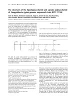
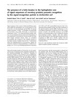
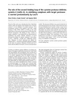
A simple quantitative criterion of buffering actionFigure 1
A simple quantitative criterion of buffering action.
(See main text for detailed explanation) A, Communicating vessels
model of partitioning processes. In a system of two communicating vessels (A and B), total fluid volume is the sum of the two
partial volumes in A and B. In an equilibrated system, the partial volumes in the individual vessels can be described as functions
of total fluid volume; these functions are termed "partitioning functions". The derivatives of the partitioning functions tell what
fraction of a total volume change is conveyed to the respective vessel. B, Partitioning of a quantity in a two-compart-
ment system. A given total change of quantity in the system produces two partial changes in compartments A and B. The
greater the partial change in B, the smaller the change in A, and the greater the "buffering" of the quantity in A. C, Partition-
ing of H

+
ions between water and buffer. Free H
+
ions are added to an aqueous solution containing a weak acid (e.g. as
strong acid). Some of the added H
+
ions remains free, some become bound to buffer molecules. C, General definition of
measures of buffering action. The differential dz/dy, paraphrased as d(buffered)/d(total), is termed the buffering coefficient b.
The differential, paraphrased as d(buffered)/d(unbuffered), is termed the buffering ratio B.
Theoretical Biology and Medical Modelling 2005, 2:8 />Page 5 of 17
(page number not for citation purposes)
other compartment. The example of communication ves-
sels also shows that the magnitude of change (when
expressed in either of these ways) is not affected by the
direction of the change: it remains the same whether the
quantity in question is added to the system, or whether it
is subtracted.
Unspectacular and intuitive as it may appear, this criterion
will lead to conclusions that differ considerably from
established views. For instance, it is usually held (on the
basis of Van Slyke's definition of buffering strength [4])
that a weak acid buffers H
+
ions most strongly when H
+
ion concentration is equal to the acid constant K
A
(i.e.,
when [H
+

] = K
A
). However, this is not where the fraction
of added H
+
ions binding to buffers is greatest. Rather, this
fraction reaches a maximum when [H
+
] approaches zero
(Figure 1C). According to our simple criterion, that is the
point of maximum buffering strength (i.e., when [H
+
] =
0). Similarly, when H
+
ions are removed from such a solu-
tion (e.g. by addition of strong base), the fraction sup-
plied via deprotonation of buffer molecules (as opposed
to a decrease of free [H
+
]) is greatest at low total [H
+
]. This
classic case illustrates the impact of the various buffering
strength units on our perception of buffering strength,
and is analyzed in detail, together with several further
examples, in the accompanying paper (Buffering II). Our
concept of buffering results, ultimately, from the system-
atic application of this simple criterion.
Deriving quantitative measures of buffering strength from this

criterion
With our simple criterion at hand, all that is left to do in
order to quantitate buffering action is to put numbers on
the magnitude of the change in the compartment that
buffers or stabilizes the other compartment (termed
"buffering compartment", corresponding to vessel B in
Figure 1A). This can be done in two equally useful ways
(Figure 1D):
Firstly, change in the "buffering compartment" can be
expressed with respect to the total change in the system.
The resulting measure represents a "fractional change",
here termed "buffering coefficient b"
The buffering coefficient b thus indicates the proportion
between one particular part and the whole.
Secondly, change in the "buffering compartment" can be
expressed with respect to the complementary change in
the other compartment, termed "target compartment" or
"transfer compartment", to indicate that one views this
compartment as the one for which the imposed change is
"intended" (corresponding to vessel A in Figure 1A). We
thus obtain a second measure, here termed the "buffering
ratio B":
The buffering ratio B thus indicates the proportion
between the two parts of a whole. This measure is com-
pletely analogous to the "odds" as used for the quantita-
tion of chance (mainly by epidemiologists) and may
therefore be termed synonymously "buffering odds B".
In the following section, we illustrate a few characteristic
types of buffering, using again fluid-filled communicating
vessels as an example (Figure 2).

Use of buffering coefficient and buffering ratio for the quantitation of
buffering action – some typical examples
A simple buffered system
Consider a system of two communicating vessels, both
having identical dimensions and constant cross sectional
areas (Figure 2A, left panel). We consider vessel A our com-
partment of interest (i.e., the "target" or "transfer
compartment"), and ask how much the fluid volume
inside it is stabilized or "buffered". To determine the
degree of buffering, we titrate the system up and down by
adding or removing fluid. We find that the volume
changes in A are always only half as big as the changes of
total volume in the system; the volume inside A is
"buffered".
The behavior of the system is repesented graphically on
the right hand of Figure 2A. Total volume is plotted on the
abscissa. The individual volumes in vessels A and B at a
given total volume are indicated in this "area plot" by the
respective heights of the two superimposed areas at that
point. Volumes inside vessel A and B are thus expressed as
functions of the independent variable "total volume". We
denote that variable by the letter x. Moreover, the volume
in the transfer vessel A expressed as a function of total vol-
ume is termed the "target function" or "transfer function",
denoted τ(x), and the volume in the buffering vessel B
expressed as a function of total volume is termed the
"buffering function", denoted β(x). "Change" in a com-
partment then can be defined more specifically as the first
derivative of the particular function with respect to the
independent variable, notated briefly as τ'(x) or β'(x).

The buffering coefficient b, defined above as the ratio of
"volume change in vessel B" over "total volume change in the
system", can then be expressed more simply and generally
as
b = β'(x)/[τ'(x) + β'(x)].
b
change in buffering compartment
total change
≡ .
B
change in buffering compartment
change in transfer compar
≡
ttment
.
Theoretical Biology and Medical Modelling 2005, 2:8 />Page 6 of 17
(page number not for citation purposes)
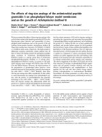
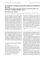
Communicating vessels as a physical model for a buffered systemFigure 2
Communicating vessels as a physical model for a buffered system.
Total fluid volume is taken as x, fluid volume inside ves-
sel A ("transfer vessel", red) as the value of the transfer function τ(x), and aggregate fluid volumes in the other vessels ("buffer-
ing vessels", blue) represent the "buffering function" β(x). We can describe these systems in terms of our two measures of
buffering action, namely the buffering coefficient b(x) = β'(x)/[τ'(x) + β'(x)] and the buffering ratio B(x) = β'(x)/τ'(x) (see main
text for detailed explanation). A, Linear buffering, one buffering vessel. The volume changes in A are only half as big as the
total volume changes in the system; the volume inside A is "buffered", or, more specifically, "moderated". The degree of mod-
eration is the same at all fluid levels; b(x) = constant = 0.5 and B(x) = constant = 1. B, Zero buffering, or perfect transfer.
Changing total volume in the system translates completely into identical volume changes in vessel A, without "moderation" or
"amplification": b(x) = 0 B(x) = 0. C, Linear buffering, several buffering vessels. Increasing the number of buffering vessels
increases buffering action. The four partitioning functions are replaced by a single buffering function β. Buffering parameters are
b(x) = 0.8 and B(x) = 4. D, Linear buffering, general case. Same buffering behavior as in C, brought about by a single buffering

vessel. E, Non-linear buffering, one buffering vessel. In this system, the individual volume changes are not linear functions of
total volume. Consequently, the proportion between volume flow into or out of vessels A is not a constant, but a variable
function of the system's filling state. F, Non-linear buffering, several buffering vessels. In most buffered systems, buffering is
brought about by a multiplicity of buffers (as in C) that are non-linear in their individual ways (as in E). Buffering coefficient and
buffering odds provide overall measures of buffering action that neither require nor deliver any knowledge about the individual
components.
Theoretical Biology and Medical Modelling 2005, 2:8 />Page 7 of 17
(page number not for citation purposes)
In this system, total change equals the sum of the individ-
ual changes (other systems are covered below), and thus
τ'(x) + β'(x) = 1,
and hence
β'(x)/[τ'(x) + β'(x)] = β'(x)/1 = β'(x).
Because the buffering function β(x) equals 0.5·x in this
system, we obtain a dimensionless buffering coefficient of
b = 0.5. In words, a buffering coefficient of 0.5 says that of
the total change imparted to the system, a fraction of 0.5
(or 50%) is directed to the "buffering compartment".
The buffering ratio B, on the other hand, which was
defined above as the ratio of "volume change in vessel B"
over "volume change in vessel A", can then be expressed as
B = β'(x)/τ'(x).
With τ(x) = β(x) = 0.5·x in this system, we find a value of
B = 1. In words, a buffering ratio of 1 says that when a
certain change is imposed to the system, the change in the
target compartment is always associated with a similar
sized change in the buffering compartment. In terms of
fluid volume: for every drop going into or out of vessel A,
another drop goes into or out of vessel B.
An unbuffered system

Figure 2B shows a system without a "buffering vessel".
Accordingly, changes in total volume are completely
translated into exactly equal changes of volume in vessel
A. Again, the point here is how to express this type of buff-
ering behavior numerically. Change in the transfer vessel
A is given by a transfer function τ(x) = x, and change in the
buffering vessel, given its non-existence or zero volume,
by a buffering function that has a constant value of zero:
β(x) = 0. We compute the buffering coefficient b again as
b = β'(x) and find that b = 0, and compute the buffering
ratio B as B=β'(x)/τ'(x) and find that B = 0. We see that
both measures yield scales with an "absolute zero", i.e.,
where the position of "zero" does not depend on some
arbitrary external reference (as would be the case with
electrical or thermodynamical potentials, for instance) or
on some similarly arbitrary convention (such as for the
Celsius scale for temperature), but follows inescapably
from the definition of the unit.
Again, it may appear trivial to find zero values for buffer-
ing strength in the absence of buffering. However, this
desirable property of a buffering strength unit is not the
rule, including the widely used H
+
buffering strength unit
introduced by Van Slyke. This unit, defined as β =
d(Strong Base)/dpH, will always be greater than zero even
in the complete absence of buffering; even stranger, the
particular numerical value representing the absence of
buffering will vary with pH (see detailed discussion in
Buffering II).

Multiple buffering vessels vs. an equivalent single one
Next, as shown in Figure 2C, we add several additional
copies of similar buffering vessels (vessels B,C,D,E). Com-
pared to a single buffering vessel B, this alteration results,
of course, in increased buffering action. When one com-
pares the initial situation with a single buffering vessel to
the system comprising four such vessels, it is reasonable to
say that buffering action increases four-fold. However, we
are not yet in a position to compute the buffering coeffi-
cient of buffering ratio.
In principle, the volumes in these vessels can be expressed
by several individual functions which may be termed
"partitioning functions". However, what matters with
respect to the stabilization or buffering of the volume in
vessel A is only their aggregate volume as a function of
total volume. This aggregate function, i.e., the four parti-
tioning functions lumped together into a single function,
represents our "buffering function β(x)". With respect to
buffering, the system in Figure 2C is thus perfectly equiv-
alent to the system in Figure 2D. In both systems, the buff-
ering function has the value of β(x) = 0.8·x, and we thus
find a buffering coefficient of b = 0.8, and a buffering ratio
of B = 4.
Indeed, the buffering ratio increases accordingly from B =
1 to B = 4. This behavior is typical for a "ratio scale", and
is a desired property. Ratio scales not only represent the
phenomena under study in a particularly intuitive way,
they are also the highest type of scale inasmuch they allow
meaningful application of the widest range of mathemat-
ical operations, including averaging, expression as per-

centage, and comparison in terms of ratios.
In contrast, the buffering coefficient changed from 0.5 to
0.8. Evidently, the buffering coefficient does not yield a
ratio scale: the four-fold increase in the number of buffer-
ing vessels is reflected in an only 1.6-fold increase of the
buffering coefficient. Another four-fold increase from 4 to
16 buffering vessels would entail an even smaller increase
of the buffering coefficient, from 0.8 to 0.94, an approxi-
mately 1.2-fold increase.
Systems exhibiting non-constant buffering
In the system depicted in Figure 2E, the cross-sectional
area of the buffering vessel is not constant, but varies with
fluid level. As a consequence, the individual volumes in
vessels A and B changes are not linear functions of total
volume of the type y = constant·x, but may be any arbi-
trary non-linear function. The proportion between the
Theoretical Biology and Medical Modelling 2005, 2:8 />Page 8 of 17
(page number not for citation purposes)
two individual changes in vessels A and B is therefore not
constant, but varies depending on the system's filling
state. The two measures of buffering action can be com-
puted exactly as indicated above as β'(x) and β'(x)/τ'(x),
respectively, but the results are valid only for the given
value of x. Consequently, buffering coefficient and buffer-
ing ratio must be presented as b(x) and B(x), respectively,
where x specifies the filling state of the system. Such vari-
able buffering is found in most buffered systems of scien-
tific interest, including buffering of H
+
and Ca

++
ions in
plasma and cytosol.
Non-constant buffering with multiple irregular buffering vessels
Figure 2F carries this more realistic version one step fur-
ther, inasmuch as buffering is also often brought about by
several different buffers each of which may be non-linear
in its own way. This situation is replicated by a combina-
tion of several, irregularly shaped buffering vessels. A buff-
ering function β(x) is again obtained by lumping together
the individual partitioning functions of the buffering ves-
sels into a single aggregate buffering function. Buffering
coefficient and buffering ratio are then computed in the
known way for a given value of x. Buffering coefficient and
buffering ratio provide overall measures of buffering
action that neither require nor deliver any knowledge
about the individual components, and many different
combinations of buffering vessels can bring about identi-
cal buffering behavior.
A formal and general definition of the approach
Systems of functions as representations of buffering phenomena
The above examples of systems of communicating vessels
(Figure 2) are useful to become familiar with our
approach to the quantitation of buffering action. Indeed,
this approach is essentially simple, and the principles
illustrated by fluid partitioning between two vessels can
be applied immediately to other quantities that distribute
between two complementary compartments, for instance
to the classical case of H
+

or Ca
++
ions in their complemen-
tary pools of "bound" and "free" ions (Buffering II).
On the other hand, these examples can illustrate only a
fraction of the things one can do in principle with this for-
mal approach to the quantitation of buffering action. This
approach has the potential to provide a common lan-
guage for all types of buffering phenomena, not just for
the few cases mentioned. The universal nature of these
measures of buffering action, and their various uses can be
appreciated and exploited best when the concept is pre-
sented in a pure mathematical form. Herein, our buffering
concept resembles other formal frameworks such as prob-
ability theory or control theory which are, at the core, of
purely mathematical nature; specific examples (e.g. flip-
ping coins or control circuit diagrams, respectively) may
illustrate these concepts, but cannnot capture them com-
prehensively and systematically.
Emphasizing those aspects that help to use this approach
as a "mathematical tool", the following paragraphs pro-
vide such a systematic framework for the quantitation of
buffering action. Herein, combinations of communicat-
ing vessels (each with its individual fluid volume depend-
ing on the common variable "total fluid volume") are
replaced by combinations of purely mathematical func-
tions of a common variable. We need the concepts of
"partitioned", "two-partitioned" and "buffered systems",
of the "sigma function" and the distinction between
"conservative" and "non-conservative" partitioned sys-

tems, between "moderation" and "amplification",
between "inverting" and "non-inverting" buffering, and
between "buffering power" and "buffering capacity".
All the definitions and concepts set up here will be
applied to specific buffering phenomena in the accompa-
nying article (Buffering II). Some interesting theoretical
aspects are presented in the Additional files. They touch
on the question "What is buffering?" (as opposed to the
question "How can we quantitate buffering?"). It will be
shown that the definition of "buffering" can be reduced to
a set of axioms in almost exactly the same way as the con-
cept of "probability", and therefore an answer to this
question is to be sought on the same spot and with the
same mathematical and philosophical approaches.
Two-partitioned systems
In a system of two communicating vessels, the individual
fluid volume in one vessel could be described as a func-
tion of total fluid volume, and the volume in the other
vessel by another function of the same total fluid volume.
We are thus dealing with two functions of a single com-
mon independent variable. More precisely, with an "unor-
dered pair" or a "combination" of functions, inasmuch as
the two functions are not in a particular order. A combi-
nation of two functions of a common independent varia-
ble is termed a "two-partitioned system", or
2
P in brief. Its
two functions are termed "partitioning functions" and
denoted π
1

and π
2
. A two-partitioned system can thus be
written
2
P = {π
1
(x), π
2
(x)}, if we let x represent the inde-
pendent variable. In the following, both functions are
assumed to be continuous and differentiable, and x, π
1
(x)
and π
2
(x) are all real valued.
Importantly, in order to use the buffering paradigm in a
meaningful and correct way, a two-partitioned system is a
necessary and sufficient condition. As a consequence, one
can apply the buffering paradigm outside pure mathemat-
ics to "real world"-phenomena provided these phenom-
ena are represented mathematically by such a
combination of functions.
Theoretical Biology and Medical Modelling 2005, 2:8 />Page 9 of 17
(page number not for citation purposes)
Conservative partitioned systems, and the "sigma function"
The examples above obeyed a conservation law, due to
physical or chemical constraints: Fluid distributed into
various compartments, but its total volume was constant;

H
+
ions added into a solution were bound by buffers or by
water, but their total number did not change. More gener-
ally, if the quantity in question is neither created or
destroyed in the process, the total change imposed onto
the system equals the sum of the two partial changes.
Analogously, in terms of functions, we use the term "con-
servative partitioned system" to designate a system of par-
titioning functions whose sum equals the value of the
independent variable. That condition, termed "conserva-
tion condition", can be written as:
[π
1
(x) + π
2
(x) + π
n
(x) ] = = x.
The "sum" of the individual functions, given by the
expression , can be used to define a function σ
(termed "sigma function") that lumps together all parti-
tioning functions π
i
of a n-partitioned system:
σ: x → .
Using this sigma function, we can rewrite the "conserva-
tion condition" briefly as σ(x) = x. Many important phe-
nomena can be represented and analyzed in terms of a
conservative partitioned system. Nonetheless, conserva-

tion (in this mathematical sense) is an accidental, not a
general feature of partitioned systems.
Non-conservative partitioned systems
We thus drop the conservation condition σ(x) = x, and
allow σ to be a continuous function of any type. This gen-
eralization will turn out to be very useful (Buffering II). On
the one hand, it allows one to express conservative sys-
tems in alternative, "parametric" form. As an example,
when one describes bound and free H
+
ions (expressed in
terms of "moles") as a function of total H
+
ions (added for
instance as strong acid), one may readily measure strong
acid in terms of "grams" or "milliliters", instead of
"moles". Then, the aggregate "output" does not equal the
"input", or σ(x) ≠ x; this inequality characterizes the sys-
tem as "non-conservative". More importantly, the concept
of non-conservative systems allows us to deal with func-
tional relationships between completely heterogeneous
physical quantities, and to apply the buffering concept to
this class of phenomena. Examples include the buffering
of organ perfusion in the face of variable perfusion pres-
sure, or systems level buffering (Buffering II).
Partitioning functions and sigma function can be repre-
sented graphically in various ways (Figure 3), e.g. as a fam-
ily of curves or by an area plot. Moreover, partitioned
systems with two partitions π
1

and π
2
can be represented
by a three-dimensional space curve . For
instance, the buffering of H
+
ions in pure water or by weak
acids is represented as space curve in the accompanying
article (Buffering II).
Buffered systems
In order to talk about buffering with respect to two com-
municating vessels, it is necessary to decide which vessel
would be considered the buffer of the other one. With
respect to H
+
ions, this assignment is conventionally made
in such a way that "free H
+
ion concentration" is said to be
buffered, and "bound H
+
ion concentration" that which
brings about buffering. More generally, the two partition-
ing functions in a two-partitioned system must be
assigned two different, complementary roles.
Which is which must be indicated explicitly; here, this
shall be done via the particular order: The first partition-
ing function is taken as description of the quantity that is
being buffered, and termed "target" or "transfer function".
For clarity, we denote the transfer function by τ(x). The

second function is taken as to describe the quantity that
brings about buffering, and is termed the "buffering func-
tion" β(x). Obviously, two partitioning functions π
1
(x)
and π
2
(x) can be arranged in two different ways, with the
resulting "ordered combinations" (or "variations") writ-
ten here {π
1
(x), π
2
(x)} and {π
2
(x), π
1
(x)}. An ordered
pair of functions is called a "buffered system". Briefly, a
buffered system B can be written B = {τ(x), β(x)}.
Quantitative parameters to describe the behavior of buffered
systems
For every x in an ordered combination of two differentiat-
able functions τ and β, there are two derivatives τ'(x) and
β'(x). The proportions between the two derivatives (i.e.,
"rates of change") serve to quantitate "transfer" (to the
"target compartment") and its complement, "buffering",
according to our simple criterion defined above. In gen-
eral, there are four ways to express the proportions
between two parts of a whole (Figure 4). Accordingly,

there are four quantitative measures of buffering or trans-
fer in a "buffered system". Herein, we also employ the
equivalences y↔τ(x) and z↔τ(x) to facilitate geometrical
interpretation in terms of partial derivatives of a space
curve (Figure 3D).
π
i
i
n
x()
=
∑
1
π
i
i
n
x()
=
∑
1
π
i
i
n
x()
=
∑
1
x

y
z
x
x
x










=










π
π
1
2

()
()
Theoretical Biology and Medical Modelling 2005, 2:8 />Page 10 of 17
(page number not for citation purposes)
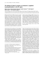
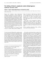
Graphical representation of two-partitioned systems of functionsFigure 3
Graphical representation of two-partitioned systems of functions.
The unordered combination of two functions π
1
(x),
π
2
(x) of a single independent variable x is termed a "two-partitioned system of functions". The two functions may represent the
two complementary parts of a whole, e.g. "bound H
+
ions" vs. "free H
+
ions" in an aqueous solution. The sum of the two func-
tions is termed "sigma function" σ(x) (see main text for detailed explanation) A, Family of curves. The individual functions π
1
(x),
π
2
(x), and σ(x) may be plotted individually as a family of curves (this is possible for multi-partitioned systems as well). B & C,
Area plots. The individual partitioning functions of partitioned systems can be plotted "on top of each other" such that the
value of each function is represented by the vertical distance between consecutive curves. In a partitioned system, their order
is not constrained, and thus two equally valid representations exist for a two-partitioned system (B,C). A limitation of area
plots is that they do not allow visualization of negative-valued partitioning functions. D, Three-Dimensional Space Curve.
The independent variable x and the values of the partitioning functions π
1
(x), π

2
(x) of a two-partitioned system may be inter-
preted as x-, y- and z-coordinates, respectively. This results in a three-dimensional space curve. Such a curve can display both
positive and negative values. Again, there are two different, equally valid representations. Projections of that curve on the xy-
plane (red) and xz-plane (blue) correspond to the individual partitioning functions π
1
(x) and π
2
(x). Projection of the space curve
on the yz-plane (gray) corresponds to a plot of the composite relations π
1
(π
2
(x)) or π
2
(π
1
(x)); these projections are not neces-
sarily single-valued functions. The projection on the yz-plane is suited particularly well to assess the proportion between the
individual rates of change of the two functions. Importantly, these proportions provide the clue to the quantitation of "buffering
action".
Theoretical Biology and Medical Modelling 2005, 2:8 />Page 11 of 17
(page number not for citation purposes)
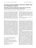
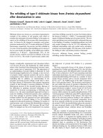
Proportions in Two-Partitioned SystemsFigure 4
Proportions in Two-Partitioned Systems.
The buffering measures are dimensionless proportions between two parts of a
whole, or between one particular part and the whole. A, Bisection of a straight line. An oriented line of length σ (row
1) can be divided in several ways into two parts of lengths τ (red) and β (blue), respectively (rows 2–5). Dividing the line at a
point that is lying on the line itself gives rise to an "inner division" (rows 2 and 3), whereas dividing the line outside the interval
yields an "outer divison" (rows 4 and 5). Proportions between the two parts can be expressed in various ways (Figure 4D).

For inner divisions, proportions are positive-valued. For outer divisions, "negative proportions" and fractional lengths greater
than 1 or smaller than 0 are obtained. B, Bisection of a function The principle of dividing a quantity into two is also applicable
to the values of a function of x at a given value of x. Thus, there are multiple ways to split an entire function σ into two func-
tions τ and β such that the sum of their values τ(x) and β(x) equals the value σ(x) for every x. C, Bisection of a slope, or rate
of change. The quantity to be bisected may as well be the slope σ' of a function σ. Again, there are multiple ways to split a
function σ into two functions τ and β such that the sum of their first derivatives τ'(x) and β'(x) equals σ'(x) for every x. For
functions and derivatives of functions alike, the proportions between the two parts into which they were split can be
expressed by the four measures indicated in Figure 4D. "Buffering" relates to the proportion between such partial rates of
change of two complementary processes. D, Measures of proportionality between the parts of a bisected slope. Propor-
tions among two partial rates of change τ' and β' that result from bisection of a whole rate σ' can be expressed either as frac-
tions of a part with respect to the whole (τ'/σ' and β'/σ') or as as ratio of one part over the other (τ'/β' and β'/τ'). The following
terminology is suggested: t, "transfer coefficient"; b, "buffering coefficient"; T, "transfer ratio"; B, "buffering ratio". These param-
eters serve to quantitate buffering action. E, Relation between the four measures of proportion. Any single one of the four
measures (t,b,T,B) fully determines the other three. The plot shows b, T, and B as functions of t. F, Trigonometric measure of
proportionality between parts of a bisected slope. The two partial rates of change τ'(x) and β'(x) may be interpreted as
two perpendicular vectors. Their resultant τ'(x) + β'(x) encloses an "buffering angle α" with τ'(x). The buffering angle and the
four buffering parameters (t, b, T, B) are related by four bijections with the buffering angle
. A buffering angle α = 0 is equivalent to zero buffering, a buffer-
ing angle of 90° to perfect buffering. This representation of buffering behavior does not have discontinuities at "infinite" transfer
or buffering odds, and is able to reflect the full range of buffering withing half a unit circle (-45° to 135°). (See Supplement 5 for
further details)
AB
AB
α:
α
αα
α
αα
α
α

α
α
tbTB=
+
=
+
==
cos
cos sin
,
sin
cos sin
,
sin
cos
,
cos
sin
Theoretical Biology and Medical Modelling 2005, 2:8 />Page 12 of 17
(page number not for citation purposes)
Transfer coefficient t
Thus, the transfer coefficient expresses the proportion
between slope of the transfer function and slope of the
sigma function, equivalent to a "fractional" slope or rate
of change (taking the slope of the sigma function as
"total" slope or rate of change). One might paraphrase the
transfer coefficient briefly as the differential
. Such a quantity is similar to terms used
in specific scientific contexts, such as "yield", "gain", or
"compliance".

Buffering coefficient b
The buffering coefficient thus expresses, analogous and
complementary to the transfer coefficient, a "fractional"
rate of change, namely that of the buffering function with
respect to the sigma function. Briefly, the buffering coeffi-
cient can be paraphrased by the differential .
By analogy to the synonyms of the transfer coefficient, one
might call the buffering coefficient also "fractional loss"
or "uncompliance".
Transfer ratio (or transfer odds) T
In words, the transfer odds reflect the proportion between
the two complementary slopes or rates of change, or the
differential . Possible synonyms roughly
matching current buffering terminology are "transfer
power" and "transfer strength".
Buffering ratio (or buffering odds) B
Thus, the buffering odds similarly reflect the proportion
between two slopes or rates of change, but expressed as
the inverse of the transfer odds: buffering function slope
over transfer function slope, or the differential
. Again, possible synonyms
corresponding roughly to current buffering terminology
are "buffering power" and "buffering strength".
Importantly, the differentials = b and
= B are useful as measures of buffering
action. They are universal and allow one to quantitate
both moderation and amplification. Moreover, the buff-
ering odds B yield the desired absolute ratio scale for buff-
ering action.
Some properties of the parameters t, b, T, and B

The four parameters are completely interdependent, and
any single one of these four parameters completely deter-
mines the other three and may be used to express the
other ones (Figure 4E and Additional file 3). The parame-
ters t, b, T, and B are defined for positive, negative and
zero-values of x, τ(x), β(x), and of the corresponding pro-
portions between their slopes. For space curves (Figure
3D), this property appears trivial. When applied in the
context of specific physical sciences, however, this prop-
erty allows one to describe buffering phenomena that
involve negative quantities or zero values. Naturally, this
is impossible to achieve with buffering strength units that
include logarithmic transforms. In principle, the concept
of "buffered systems" can be adapted easily to situations
where the system state depends not on one single param-
eter, but on several of them (Additional File 3).
Turning the basic approach into a systematic framework
Categories of buffered systems
Classification according to local behavior
We propose to use the term "buffering" as a general term
for all types of behavior of buffered systems. In contrast,
the terms "moderation" and "amplification" shall denote
specific types of behavior of such systems; namely, "mod-
eration" for buffering with |t(x)| < 1, and "amplification"
for buffering with |t(x)| > 1. Furthermore, we can distin-
guish "inverting buffering" for which t<0, from "non-
t(x)
dy
dx
dy

dx
dz
dx
x
xx
≡












+






=
+






τ
τβ
’( )
’( ) ’( )

=






∈
()
τ
σ
’( )
’( )
x
x
tR
d (transferred)
d (total)
b(x)
dz
dx
dy
dx

dz
dx
x
xx
≡












+






=
+






β
τβ
’( )
’( ) ’( )

=






∈
()
β
σ
’( )
’( )
x
x
bR
d (buffered)
d (total)
T(x)
dy
dx
dz
dx
x

x
TR≡












=






∈
()
τ
β
’( )
’( )
d (transferrred)
d (buffered)
B(x)

dz
dx
dy
dx
x
x
BR≡












=






∈
()
β
τ

’( )
’( )
d (buffered)
d (transferrred)
d (buffered)
d (total)
d (buffered)
d (transferrred)
Theoretical Biology and Medical Modelling 2005, 2:8 />Page 13 of 17
(page number not for citation purposes)
inverting buffering" for which t>0. Combining these two
criteria, one can distinguish "inverting amplification",
"inverting moderation", "non-inverting moderation",
and "non-inverting amplification". All classical chemical
buffers (e.g. for H
+
, Ca
++
or other ions) are "non-inverting
moderators".
Classification according to global behavior
In addition to the classification by local buffering behav-
ior, one may distinguish buffered systems according to
their behavior over the entire definition range. Thus, "lin-
ear buffers" have transfer and buffering functions that are
linear functions of the type τ(x) = a
1
·x + b
1
, and β(x) =

a
2
·x + b
2
, where a
1
,a
2
,b
1
,b
2
are constants. For a linear
buffer, the proportion between the two partitions is fixed,
and the buffering properties are therefore the same at all
states of the system. Examples are the partitioning of fluid
between two cylindrical vessels (Figure 2A–D), partition-
ing of a solute between the two phases in an oil/water
emulsion, or taxation according to a fixed tax rate.
"Nonlinear buffers" have nonlinear buffering functions of
any other type, and thus the proportion between the two
partitioning functions varies with x. Thus, the buffering
properties of nonlinear buffers depend on the system
state, or the value of the independent variable. Examples
include the partitioning of fluid between two irregularly
shaped vessels (Figure 2E–F), the buffering of H
+
ions by
water or by weak acids or bases (Buffering II), and taxation
according to a progressive tax rate.

Buffering capacity vs. buffering power
For the sake of clarity, we would further like to maintain
the distinction between intensity terms and capacity terms in
the quantitative description of buffering. As differentials,
the parameters t, b, T, and B are intensity terms which
describe "fractional rates of change" or "proportions
between rates of change". In contrast, a genuine capacity
term reflecting an absolute change is obtained by defining
a "buffering capacity" C
B
as the difference between two par-
ticular values z
1
and z
2
of the buffering function:
"buffering capacity" C
B
≡ ∆z = z
2
- z
1
= β(x
2
) - β(x
1
).
A "transfer capacity" C
T
can be defined analogously as the

difference between two particular values y
1
and y
2
of the
transfer function. These "capacities" are either dimension-
less numbers, or they are of the same dimension as y and
z. For instance, acid-base physiologists and clinicians use
the term "total body bicarbonate deficit" (TBBD) in this
sense to denote the absolute amount of bicarbonate (indi-
cated in moles or grams) that is needed to increase the
present low pH of a patient with metabolic acidosis to the
normal value of 7.4.
Visualizations: communicating vessels, space curve, buffering angle
Visualizing the elementary partitioning processes that
underlie the buffering phenomena not only has great
didactic value, but can as well provide a clear and simple
representation of buffering phenomena of genuine scien-
tific interest and that are otherwise complicated or
abstract; this may help to avoid or to correct misconcep-
tions. Lack of such direct visual equivalents may have con-
tributed to misconceptions and confusion associated with
existing buffering strength units in the past [5,6], and to
the persisting difficulties of students with that subject.
Fluid-filled communicating vessels can replicate exactly
the buffering behavior of virtually all "classical" buffering
phenomena, and thus provide visible and tangible "class-
room models". In Figure 2, we used this model to illus-
trate the practical use of the buffering parameters t, b, T,
and B. A general method to construct communicating ves-

sel-models of arbitrary buffered systems is described in
Additional file 4. The models may be designed in a way
that they not only replicate the elementary partitioning
process, but also directly visualize buffering strength in
terms of the buffering ratio B (or any other buffering
parameter, if desired).
Three-dimensional space curves are a more general way to
represent two-partitioned and buffered systems graphi-
cally (Figure 3D). When such a space curve is projected
parallel to the x-axis onto the yz-plane (defined by the two
axes that are used to represent τ(x) and β(x), respectively),
then a tangent to the curve will enclose a certain angle α
with the τ-axis. This "buffering angle" provides another
visualization of the proportion between τ'(x) and β'(x)
and has useful mathematical properties, analogous to the
use of trigonometric representations used in electrical
engineering (see Additional file 5 for details, and Figure
4F).
Axiomatic foundation
The measures of buffering introduced in this article
(t,b,T,B) are essentially proportions between two ele-
ments, albeit with some additional specifications: i) The
elements form an ordered pair; ii) The elements and their
proportions are not fixed, but may vary as a function of
some independent variable; and iii) The elements are rates
of change (here: derivatives of differentiable functions).
Figure 4 illustrated some basic aspects of proportions,
including "negative proportions", and various ways to
represent such proportions.
In a way, our concept is thus a "play" on proportions, and

like any game, it is played in accordance with certain rules.
Here, elements and rules are purely mathematical objects.
For theoreticians, this situation is an invitation to build
the buffering concept from scratch on a minimal set of
Theoretical Biology and Medical Modelling 2005, 2:8 />Page 14 of 17
(page number not for citation purposes)
postulates or axioms. For scientific practitioners, motiva-
tion to found the concept of buffering on axioms may
spring from the experience that seemingly diverse phe-
nomena may be governed by identical principles, and that
these more abstract principles allow all of them to be han-
dled with a single mathematical tool. In this sense, Addi-
tional file 6 is an attempt to demonstrate the common
principle behind "buffering", "partitioning", and "proba-
bility" in an intuitive way, and to point out the desired
properties of an axiomatic formulation of these
principles.
Additional file 7 then presents such an axiomatic formu-
lation of "buffering" or "partitioning" or "probability".
These axioms represent the most concise, definitive, and
versatile version of our buffering concept. For many
readers, it will also offer the most direct approach, espe-
cially if they are already familiar with Kolmogorov's axio-
matic foundation of a probability measure.
Importantly, the axiomatic foundation makes the theoret-
ical concept more powerful: Firstly, stringent formaliza-
tion allows one to decide definitively whether the concept
is logically consistent and complete. Secondly, axioms
represent the concept in its most general form, and this
form is most likely to stimulate free (and correct) use in

very diverse, sometimes unanticipated contexts. Moreo-
ver, systems of continuous functions are adequate only for
a macroscopic description of buffering phenomena. On a
microscopic scale, the continuum hypothesis ceases to
apply, whereas the quantitative principles that govern
these phenomena remain the same. The axioms therefore
also provide for systems of discrete functions.
Finally, the axiomatic form exposes the striking formal
similarity between the concepts of "probability" and of
"buffering" (detailed in Tables 3 and 4 of Additional file
7). This similarity raises deep questions -remaining to be
explored- regarding both the interpretation and the math-
ematical foundation of "probability".
Interconversions and practical rules
The general form of the axioms allows one to identify sev-
eral "technical" aspects of buffered systems that are prac-
tically relevant. Firstly, there exist equivalencies with
respect to buffering properties between systems that
present initially in very different forms. Understanding
these equivalencies and being able to interconvert such
systems allows one to reduce complexity (Additional file
8). Secondly, buffering phenomena can be formalized as
partitioned and buffered systems in more than one, for-
mally correct way. The various options at this step allow
one to choose the most suitable formalization, and point
to some efficient experimental approaches (Additional
file 9).
Practical applications
Practical relevance and use of the concept are worked out
in the accompanying paper (Buffering II), where we apply

our definitions and units to various buffering phenomena
of genuine scientific interest. These analyses offer some
fresh though compelling looks on "classical" buffering
phenomena (H
+
buffering by pure water or by solutions of
weak acids/bases), and demonstrate that our concept
affords rigorous quantitative treatment of "non-classical"
buffering phenomena for which useful measures of buff-
ering strength have been unavailable so far (redox
buffering and blood pressure buffering). Finally, a gener-
alization opens the concept to non-stationary systems and
thus allows one to quantitate time-dependent buffering,
or "muffling", and "systems level buffering" in an equally
rigorous manner.
Discussion
The introduction of suitable abstractions is our only mental aid
to organize and master complexity. – Edsger W. Dijkstra
In this article, we introduced quantitative measures of
buffering action based on a purely mathematical concept
of "buffering". The nucleus of the concept was to describe
partitioning processes by means of the proportions
between partial and total "changes" or "flows". On this
basis, we could define four interrelated, dimensionless
measures: transfer coefficient t, buffering coefficient b,
transfer ratio T, and buffering ratio B. Together, they allow
one to quantitate the behavior of buffered systems in a
way that is analogous to the quantitation of chance using
"probabilities" and "odds". The magnitude of buffering
action may thus be measured using the "buffering coeffi-

cient" which provides a relative scale normalized to 1.
Alternatively, one may use the "buffering ratio" in order to
quantitate buffering action by means of an absolute scale
with equal intervals and an absolute zero, the highest
scale type possible.
"Buffering" according to this definition turned out to be
an entirely mathematical concept. Phenomena encoun-
tered in the "real world" may or may not be related to this
mathematical concept in exactly the same way in which
phenomena may or may not be related to mathematical
concepts in general. The concept of exponential decay, for
instance, can be stated in purely mathematical terms, but
is also exhibited in more or less perfect form by several
natural phenomena, such as decaying radioisotopes or
chemical reactions on their way to equilibrium. Moreover,
our mathematical concept of buffering can also describe
amplification phenomena, just as the concept of expo-
nential decay can seamlessly turn into a concept of expo-
nential growth simply by allowing for exponents greater
than one.
Theoretical Biology and Medical Modelling 2005, 2:8 />Page 15 of 17
(page number not for citation purposes)
This section discusses the intrinsic, formal properties of
the concept. Some of its – sometimes hidden – connec-
tions to previous work, especially to ideas of Henderson,
Van Slyke, or Neher & Augustine are exposed and dis-
cussed in Additional file 10. Kolmogorov's axiomatic sys-
tem of probability has been covered extensively elsewhere
(see literature in [7,8]). The technical and theoretical
implications of our "Non-Kolmogorov probability meas-

ure" require further study, but cannot be worked out here.
Detailed treatments of specific buffering phenomena are
presented in the accompanying paper (Buffering II).
Properties and significance of the general, formal
approach to the quantitation of buffering action
The introduction and Additional file 2 listed a number of
major problems associated with the present approaches to
the quantitation of buffering action. Our formal, general
approach and the four buffering parameters t, b, T, and B,
provide a theoretically rigorous and practically useful
solution to these problems.
A ratio scale for buffering strength
The buffering odds B provide an absolute, dimensionless
ratio scale for buffering action. This is the highest possible
type of scientific scale. The advantages of ratio scales, i.e.,
equal interval scales with an absolute zero, have been
pointed out in the introduction and in Additional file 2.
Our buffering strength scale is free of scale artefacts and
can be used accurately, not just approximately, for small
and large, positive and negative values alike. A further
benefit gained with a ratio scale is the possibility to build
simple, intuitive models of buffering, e.g. with communi-
cating vessels. Of the previous units for buffering strength,
only Neher & Augustine's "Ca
++
binding ratio κ
s
" yields a
ratio scale.
A universal scale for buffering strength

Our definitions of buffering and of measures to quantitate
buffering are purely formal, mathematical ones, and the
measures t, b, T, and B are all dimensionless numbers.
Therefore, this conceptual framework is generally applica-
ble and not arbitrarily limited to buffering phenomena of
a particular chemical or physical nature. The concept
allows one to handle all classical examples of buffering,
such as Ca
++
or H
+
buffering. In addition, it can be applied
to multiple further buffering phenomena encountered in
chemistry, biology, physiology, or elsewhere. Application
of our concept to familiar examples shows that it is valid,
i.e., it reflects faithfully what is qualitatively understood
by the word "buffering", and that this will hold generally,
not only when certain boundary conditions are met.
We stress the formal aspect of buffering: "Buffering" is a
quantitative pattern abstracted from "real" things, not a
real thing itself. Therefore, this pattern can be employed
freely and in various ways as a tool for the quantitative
description of certain aspects of reality. Whether some-
thing is the buffer or that which is being buffered is a mat-
ter of perspective and thus determined by the analyst, not
by reality. Therefore, the definition of a buffer is an oper-
ational one: Something that is expressed in terms of a
buffering function β constitutes, by definition, a buffer.
Conversly, something that cannot be measured by these
units cannot and should not be described in terms of buff-

ering terminology. Such an operational definition
requires a general, formal concept. In contrast, buffering
strength units that are specific for H
+
, Ca
++
, or other
particular entities can hardly be wrought into a convinc-
ing operational definition of buffering that is not overly
exclusive and limited.
A scale for moderation and amplification
The mathematical notation of our buffering concept
makes it easy to recognize the common pattern behind
"moderation" and "amplification", and to accommodate
this union formally. A single unit is sufficient to deal with
both, and such a unit is also called for frequently when
both types of buffering behavior occur in a single system.
The association of "buffering" exclusively with "attenua-
tion" or moderation, and the resulting mental divide with
respect to the treatment of attenuation vs. amplification
phenomena may be related to the historical roots of the
buffering concept in acid-base chemistry where "modera-
tion" is the most prominent finding. Overcoming that
divide greatly enhances the usefulness of the buffering
concept. For instance, we can connect our buffering con-
cept directly to systems and control theory, as detailed in
the accompanying article (Buffering II). This link can
enrich systems and control theory by providing a cur-
rently lacking rigorous definition of "systems level buffer-
ing" and an accompanying unit to measure this quantity.

On the other hand, this link can expand the application
range of the buffering concept to all objects and phenom-
ena already studied by systems and control theory. Most
importantly, our approach brings together conceptually
and technically "buffering" as a homeostatic mechanism,
and control theory as the dominant formal language for
the description of homeostasis in physiological systems.
A standard scale for buffering strength?
The parallel use of multiple, incommensurate scales for
buffering strength has engendered ambiguous terminol-
ogy, misunderstandings and pseudo-problems. Homo-
nymic usage of the term "buffering" might be avoided by
agreeing on a certain convention. Ideally, such a conven-
tion should codify not just any usage, but the one that
affords the highest possible type of scale. Furthermore, a
standard scale should cover all possible cases of buffering,
and should not arbitrarily exclude some of them. Our
concept constitutes such an all-purpose yardstick for buff-
Theoretical Biology and Medical Modelling 2005, 2:8 />Page 16 of 17
(page number not for citation purposes)
ering strength. It is a valid measure of buffering, univer-
sally applicable, and yields a scale of the highest possible
type. No other buffering strength unit satisfies these
requirements.
Moreover, it is also hard to imagine a more compelling,
less arbitrary standard scale than an "absolute ratio scale"
as provided by the buffering odds B: The numerical value
of the buffering odds B is completely determined by the
general definition of B as the ratio of two derivatives and
does not depend on any arbitrary scaling factors or units.

In contrast, for instance, the definition of the unit β
H+
=
dBase/dpH includes a number of additional, unnecessary
"rules" that need to be observed in order to obtain the cor-
rect value: i) Express the concentration of strong base and
of free H
+
ions in multiples of Avogadro's number per liter
(as opposed to absolute numbers, mass, or others); ii)
Carry out a numerical transformation of one quantity
([H
+
]
free
into pH), but not of the other ([Strong Base]); iii)
For the transformation, choose a logarithmic one (as
opposed to other transformations, e.g. exponential ones);
and iv) Use the number 10 as the base in this transform
(as opposed to e or any other). These procedures are all
mere conventions, not compelling formal constraints or
the results of particular scientific givens. Another example
is de Levie's redox buffer strength which includes multipli-
cation by a factor 1/ln(10) for sheer convenience [9].
Conclusion
The quantitation of chance can be achieved cleanly and
comprehensively by using either probabilities (of occur-
rence and non-occurrence of an event) or odds (for and
against an event). The analogous measures proposed in
this article, namely the coefficients (transfer coefficient t

and buffering coefficient b) and ratios (transfer ratio T and
buffering ratio B), are suited to serve as standard units for
buffering action.
Additional material
Acknowledgements
This work was inspired by a stay in the lab of Walter F. Boron, Dept. of
Cellular Molecular Physiology, Yale University, New Haven, CT, USA
Additional File 1
Current Usage of the "Buffering" Paradigm Outside Acid-Base Chemistry
Click here for file
[ />4682-2-8-S1.pdf]
Additional File 2
Problems with the Current Approaches to the Quantitation of Buffering
Click here for file
[ />4682-2-8-S2.pdf]
Additional File 3
Properties of the Parameters t, b, T, and B
Click here for file
[ />4682-2-8-S3.pdf]
Additional File 4
Constructing Communicating Vessel-Models of Partitioned and Buffered
Systems
Click here for file
[ />4682-2-8-S4.pdf]
Additional File 5
A Trigonometric Representation of Buffering Behavior: The "Buffering
Angle"
Click here for file
[ />4682-2-8-S5.pdf]
Additional File 6

From Galton Desk to Communicating Vessels – "Partitioning" as a Com-
mon Pattern Behind Probability and Buffering
Click here for file
[ />4682-2-8-S6.pdf]
Additional File 7
Axiomatic Foundation of the Formal & General Approach
Click here for file
[ />4682-2-8-S7.pdf]
Additional File 8
Conservative and Non-Conservative Partitioned Systems – Equivalences
and Interconversions
Click here for file
[ />4682-2-8-S8.pdf]
Additional File 9
Some Useful General Principles Regarding the Practical Application of the
Formal & General Buffering Concept
Click here for file
[ />4682-2-8-S9.pdf]
Additional File 10
Historical Note: Origins of the Formal & General Approach
Click here for file
[ />4682-2-8-S10.pdf]
Publish with BioMed Central and every
scientist can read your work free of charge
"BioMed Central will be the most significant development for
disseminating the results of biomedical research in our lifetime."
Sir Paul Nurse, Cancer Research UK
Your research papers will be:
available free of charge to the entire biomedical community
peer reviewed and published immediately upon acceptance

cited in PubMed and archived on PubMed Central
yours — you keep the copyright
Submit your manuscript here:
/>BioMedcentral
Theoretical Biology and Medical Modelling 2005, 2:8 />Page 17 of 17
(page number not for citation purposes)
References
1. Michaelis L: Die Wassserstoffionenkonzentration 2nd edition. Berlin,
Verlag von Julius Springer; 1922.
2. Roos A, Boron WF: The buffer value of weak acids and bases:
origin of the concept, and first mathematical derivation and
application to physico-chemical systems. The work of M.
Koppel and K. Spiro (1914). Respir Physiol 1980, 40:1-32.
3. Henderson LJ: Das Gleichgewicht zwischen Basen und Säuren
im tierischen Organismus. Ergebnisse der Physiologie 1909,
8:254-325.
4. Van Slyke DD: On the measurement of buffer values and on
the relationship of buffer value to the disociation constant of
the buffer and the concentration of the buffer solution. J Biol
Chem 1922, 52:525-570.
5. Goldsmith DJ, Hilton PJ: Relationship between intracellular pro-
ton buffering capacity and intracellular pH. Kidney Int 1992,
41:43-49.
6. Saleh AM, Rombola G, Batlle DC: Intracellular H
+
buffering
power and its dependency on intracellular pH. Kidney Int 1991,
39:282-288.
7. Primas H: Basic elements and problems of probability theory.
J Scientific Exploration 1999, 13:579-613.

8. Khrennikov AY: Interpretations of probability and their p-adic
extensions. Theory Probab Appl 1998, 46:256-273.
9. de Levie R: Redox Buffer Strength. J Chem Ed 1999, 76:574-577.
10. Schmitt BM: The quantitation of buffering action II. Applic-
tions of the formal & general approach. Theor Biol Med Model
2005, 2:9.