Báo cáo y học: "The quantitation of buffering action II. Applications of the formal & general approach" ppsx
Bạn đang xem bản rút gọn của tài liệu. Xem và tải ngay bản đầy đủ của tài liệu tại đây (710.3 KB, 15 trang )
BioMed Central
Page 1 of 15
(page number not for citation purposes)
Theoretical Biology and Medical
Modelling
Open Access
Research
The quantitation of buffering action II. Applications of the formal &
general approach
Bernhard M Schmitt*
Address: Department of Anatomy, University of Würzburg, 97070 Würzburg, Germany
Email: Bernhard M Schmitt* -
* Corresponding author
Abstract
Background: The paradigm of "buffering" originated in acid-base physiology, but was subsequently
extended to other fields and is now used for a wide and diverse set of phenomena. In the preceding
article, we have presented a formal and general approach to the quantitation of buffering action.
Here, we use that buffering concept for a systematic treatment of selected classical and other
buffering phenomena.
Results: H
+
buffering by weak acids and "self-buffering" in pure water represent "conservative
buffered systems" whose analysis reveals buffering properties that contrast in important aspects
from classical textbook descriptions. The buffering of organ perfusion in the face of variable
perfusion pressure (also termed "autoregulation") can be treated in terms of "non-conservative
buffered systems", the general form of the concept. For the analysis of cytoplasmic Ca
++
concentration transients (also termed "muffling"), we develop a related unit that is able to faithfully
reflect the time-dependent quantitative aspect of buffering during the pre-steady state period.
Steady-state buffering is shown to represent the limiting case of time-dependent muffling, namely
for infinitely long time intervals and infinitely small perturbations. Finally, our buffering concept
provides a stringent definition of "buffering" on the level of systems and control theory, resulting
in four absolute ratio scales for control performance that are suited to measure disturbance
rejection and setpoint tracking, and both their static and dynamic aspects.
Conclusion: Our concept of buffering provides a powerful mathematical tool for the quantitation
of buffering action in all its appearances.
Introduction
In the preceding article (Buffering I ), we presented a for-
mal and general framework for the quantitation of buffer-
ing action. The purpose of the present article is to apply
that mathematical tool to the analysis of some scientifi-
cally important buffering phenomena.
Recall that we formulated buffering phenomena as the
partitioning of a quantity into two complementary com-
partments, and then used the proportions between the
respective flows as a simple quantitative criterion of buff-
ering strength. The two measures of buffering action were
i) the buffering coefficient b, defined as the differential
d(buffered)/d(total), and ii) the buffering ratio B, defined
as the differential d(buffered)/d(unbuffered). Moreover,
the following analyses will make use of the distinction
between various categories of buffered systems (e.g. con-
servative vs. non-conservative partitioned systems), and
Published: 16 March 2005
Theoretical Biology and Medical Modelling 2005, 2:9 doi:10.1186/1742-4682-2-9
Received: 26 August 2004
Accepted: 16 March 2005
This article is available from: />© 2005 Schmitt; licensee BioMed Central Ltd.
This is an Open Access article distributed under the terms of the Creative Commons Attribution License ( />),
which permits unrestricted use, distribution, and reproduction in any medium, provided the original work is properly cited.
Theoretical Biology and Medical Modelling 2005, 2:9 />Page 2 of 15
(page number not for citation purposes)
will exploit the equivalencies and interconversions
between these categories.
To begin, we revisit a classical case of acid-base buffering:
H
+
ion buffering in a solution of a weak acid. This process
can be described easily in terms of a conserved quantity
(total H
+
ions) that partitions into two complementary
compartments or states (bound vs. free). Such a system
was termed a "conservative buffered system". Conserva-
tive buffered systems constitute the most simple buffered
systems according to our buffering concept, and they pro-
vide a suitable framework to describe further classical
buffering phenomena. An important one among them,
the so-called "self-buffering" of H
+
ions in pure water, is
analyzed in Additional file 2.
The concept of a "conservative buffered system" can be
applied readily and fruitfully to numerous buffering phe-
nomena that involve quantities other than H
+
or Ca
++
ions
("non-classical" buffering phenomena). Some examples
are presented in the Additional file 3; these include a
straightforward approach to the notoriously difficult
quantitation of "redox buffering", and examples which
demonstrate that the concept of "buffering" is by no
means limited to the natural sciences.
In the second section, we analyze the buffering of organ
perfusion in the face of variable blood pressure. Here, the
independent variable is blood pressure, whereas the
dependent variables are volume flows. Systems that
involve different physical dimensions, however, cannot
be formalized in terms of "conservative buffered systems",
the basic form of our buffering concept. Here, the general
form of our buffering concept (Buffering I ) proves to pro-
vide a rigorous and reliable framework for the treatment
of such "non-conservative" and "dimensionally heteroge-
neous" buffered systems.
The third section extends the buffering concept to time-
dependent buffering processes. "Time" as a potentially
important aspect of buffering becomes evident, for
instance, in the Ca
++
concentration transients that are elic-
ited by the brief openings of a calcium channel in the sur-
rounding cytoplasm [1]. It was an important achievement
to realize that this blunting of concentration swings repre-
sents an independent quantity, and to suggest a term as
fitting as "muffling" for it [2]. However, for reasons
detailed in Additional file 5, the available units of "muf-
fling strength" are not satisfying. We introduce an exten-
sion of our buffering concept that clearly satisfies all
criteria required for a muffling strength unit and provides
a dimensionless ratio scale for this quantity. Furthermore,
this unit is able to connect "muffling" and "buffering"
both conceptually and numerically: Steady-state buffering
is shown to represent the limiting case of time-dependent
muffling for infinitely long time intervals and infinitely
small perturbations.
Finally, Additional file 6 sketches how our concept of
buffering can serve to quantitate "systems level buffering"
in the context of control systems. Buffering is an impor-
tant aspect of homeostasis in physiological systems, and
control theory provides a powerful general language to
describe homeostatic processes. So far, however, the con-
cept of buffering could not be accomodated explicitly in
this framework. We show that "buffering" and "control
theory" can be connected conceptually and numerically in
a straightforward and meaningful way. To quantitate sys-
tems level buffering, we need to exploit simultaneously all
possibilities and features of our buffering concept,
because control systems may be conservative or non-con-
servative, dimensionally homogeneous or heterogeneous,
and time-invariant or time-dependent.
The buffering of H
+
ions by weak acids or bases –
Buffering as partitioning of a conserved quantity
and the concept of "Langmuir buffering"
Weak acids in conjunction with their conjugate base, and
weak bases in conjunction with their conjugate acids, are
the prototypical "buffers". They were the first buffers put
to action by biochemists in order to stabilize the pH of
solutions, and they were also the first buffers to receive
thorough theoretical analysis. Numerous textbook defini-
tions explicitly equate "buffers" with "mixtures of weak
acids plus conjugate base" (or vice versa), and this notion
became so inextricably woven into our thinking about
buffering that the distinction between the chemical sub-
strate of this process and the abstract quantitative pattern
manifest in it fell into oblivion.
In a wider sense, however, the manifold varieties of ligand
binding are indeed responsible for a large number of buff-
ering phenomena encountered in biochemistry or physi-
ology. For instance, ions such as Ca
++
are buffered by
physico-chemical processes analogous to H
+
buffering,
albeit without the involvement of literal weak acids or
bases. Compared to buffering involving other mecha-
nisms, such as blood pressure buffering or systems level
buffering (see below), buffering via ligand binding exhibits
some distinct quantitative patterns. The terminology of
the original acid-base concept of buffering, however, is
too specific as to serve as a general framework for the treat-
ment of these phenomena.
The following section demonstrates how the quantitative
patterns of buffering via ligand binding can be caught
with the aid of the four parameters t, b, T, and B. The anal-
ysis explores the classic case of a weak monoprotic acid
dissolved in water.
Theoretical Biology and Medical Modelling 2005, 2:9 />Page 3 of 15
(page number not for citation purposes)
Mathematical model of free and bound H
+
ion
concentrations in a solution of a weak acid
To obtain an explicit quantitative description of buffering
by weak acids, we first recapitulate the mathematical
model that describes the concentrations of H
+
ions in an
aqueous solution of a weak acid as a function of free H
+
ion concentration. Subsequently, we reformulate the con-
centrations of free and bound H
+
ions as functions of total
H
+
ion concentration, and combine these functions into a
buffered system. Finally, we derive the four parameters t,
b, T, and B from this system.
A weak monoprotic acid HA can dissociate into a free H
+
ion and a conjugated base A
-
, to an extent that is dictated
by K
A
, the acid constant in water, according to:
K
A
× [HA] = [H
+
]
free
× [A
-
]
free
.
The total amount of weak acid [A]
total
equals the sum [A
-
]
free
+ [HA] of dissociated and undissociated weak acid; the
system is "conservative". We can therefore substitute [A
-
]
free
by [A]
total
- [HA] and obtain:
and after several intermediate steps:
For the sake of readability, we express the same relation-
ship in a more general notation:
where c and d stand for the constants [A]
total
and K
A
,
respectively, and the variables y and z correspond to
[H
+
]
free
and [HA], respectively. This latter equation
describes a hyperbola that approaches c as y increases to
infinity. It was first used empirically by Hill [3], but
became a much more meaningful mathematical model
after Langmuir had supplied a mechanistical interpreta-
tion, namely in terms of non-cooperative binding of a lig-
and to a finite number of binding sites [4]. That model is
widely applicable to numerous phenomena, e.g. receptor-
ligand interactions, adsorption processes at surfaces, or
enzyme kinetics, to name but a few. The same rules of
non-cooperative binding apply to the binding of H
+
ions
to the conjugate base of a monoprotic weak acid.
In order to move from specific acid-base terminology to a
general ligand binding terminology, we re-interpret the
symbols in the equation as follows: Variable z
represents the concentration of bound ligand, y the con-
centration of free ligand, c the total number of binding
sites, and d the equilibrium constant K
d
of the complex
with respect its dissociation products.
"Langmuir buffers"
So far, we have described bound ligand z as a function of
free ligand y. Next, we express the concentration of free
ligand y as a function of total ligand x = y+z:
and the concentration of bound ligand z as a function of
total ligand x:
The relation between total, free, and bound ligand for
non-cooperative binding to a fixed number of binding
sites with similar affinity is shown in Figure 1A. It is easy
to double-check that the sum y(x)+z(x) equals x, i.e., the
conservation condition is satisfied.
To turn these two functions into a "buffered system", we
assign the role of "transfer function" τ(x) to the free H
+
concentration y(x), and the role of "buffering function"
β(x) to the bound H
+
concentration z(x). Because many
common and important systems follow this quantitative
pattern, it might be useful to have a specific term to refer
to them. We suggest the term "Langmuir-type buffers" or
"Langmuir-type buffered systems". Briefly, a Langmuir-type
system can be defined as an ordered pair of two functions
{y = τ(x), z = β(x)} that satisfies the three conditions (x =
y+z) and z = c × y/(d+y) and c, d ∈
+
.
In systems that involve ion concentrations, both τ(x) and
β(x) naturally assume a value of zero at x = 0, i.e., they
pass through the origin. However, we can relax this fourth
constraint by allowing for offsets τ
0
and β
0
, respectively,
without altering the buffering properties (Buffering I ).
Thus, we obtain the general form of a Langmuir buffer
B
Langmuir
as:
The buffered system constituted by the solution of a weak
acid in water is "dimensionally homogeneous": the varia-
bles x, y, and z are either all dimensionless (e.g. when
[][]
[]
HA H
[A] -[HA]
K
[H ] A [H
free
total
A
free total
=×
=
×−
+
++
]] HA
K
free
A
×
[]
,
[]
[] [ ]
[]
.HA
AH
KH
total free
Afree
=
×
+
+
+
z
cy
dy
=
×
+
z
cy
dy
=
⋅
+
y(x)
x
cd cd xcd x=+⋅+− + − −+
2
1
2
1
2
2
22
() () ()
z(x)
x
cd cd xcd x=−⋅++ + − −+
2
1
2
1
2
2
22
() () ()
\
B free,bound x
x
cd cd xcd
Langmuir
:{ }{() () () ()==+⋅+− +−−+τ
2
1
2
1
2
2
2
xx
x
x
cd cd xcd x
2
0
22
0
2
1
2
1
2
2
+
=−⋅++ + − −+ +
τ
ββ
;
() () () () }
Theoretical Biology and Medical Modelling 2005, 2:9 />Page 4 of 15
(page number not for citation purposes)
Buffering via non-cooperative ligand binding: "Langmuir buffering"Figure 1
Buffering via non-cooperative ligand binding: "Langmuir buffering"
. The prototype of Langmuir buffering is the buffering
of H
+
ions in a solution of a weak acid. A, Relation between the three variables of a "Langmuir"-type buffer. Concentra-
tions of free ligand (red), bound ligand (blue), and total ligand in a solution of a weak acid. The relations between the three var-
iables are computed from the equation , where K
d
stands for the dissociation constant of the buffer-
ligand complex, and [buffer] for total buffer concentration. [buffer] and K
d
are assumed to be constant. Plotted for [buffer] = 5
and K
d
= 1. B, Describing "Langmuir buffering" using the four buffering measures t, b, T, and B. Titration of a "Langmuir
buffer" with increasing concentrations of ligand; constant parameters are: [buffer] = 100, K
d
= 10, arbitrary concentration units.
Characteristic system states shown are the "half-saturation point" of buffer (asterisk), the "equipartitioning point" where half of
the added ligand remains free, and the other half is bound by the buffer (open circle), and the "break even point" where the lig-
and inside the system is half bound, half free (closed circle). Top panel, left: Transfer function τ, i.e., free ligand concentration (ordi-
nate) as a function of total ligand (ordinate). Top panel, right: buffering function β, i.e., bound ligand concentration as a function of
total ligand. Middle panel, left: Transfer coefficient t, i.e., the (differential) fraction of added ligand that enters the pool of free lig-
and. Middle panel, right: Buffering coefficient b, i.e., the (differential) fraction of added ligand that becomes bound to buffer. Bot-
tom panel, left: Transfer ratio T = d(free)/d(bound), i.e., the differential ratio of additional free ligand over additional bound
ligand. Bottom panel, right: Buffering ratio B = d(bound)/d(free), i.e., the differential ratio of additional bound ligand over addi-
tional free ligand. The parameters b and B provide two complementary measures of buffering strength. C, Buffering strength
of a Langmuir buffer as a function of both total ligand concentration and affinity. Wireframe surface: The buffering ratio
B is shown on the vertical axis; affinity expressed as 1/K
d
; concentration of ligand, [ligand], and K
d
in arbitrary concentration
units. Contours on bottom: Lines connect states of identical buffering strength. For a buffer with a given K
d
, buffering strength
decreases monotonically with increasing ligand concentration. However, at a fixed ligand concentration, buffering strength as a
function of affinity runs through a maximum. D, Visualizing Langmuir buffering by two-dimensional plots (same data as in
Figure C). Left hand, linear plot; white lines, states of identical buffering strength; black lines, states of identical fractional buffer
saturation. Right, double-logarithmical plot. black lines, states of identical buffering strength; red lines, states of identical fractional
buffer saturation. E, Using the "buffering angle" to visualize Langmuir buffering: cylinder plot. As shown in Buffering I, the
specific angle α for which [α = arccos(T) and α = arctan(B)] can unambiguously represent the buffering parameters t(x), b(x),
T(x) and B(x) at a given point on the x axis. Consequently, a curve on the surface of a unit cylinder can represent the buffering
behavior for an entire range of x values, yielding a "state portrait". State portraits of several Langmuir buffers are shown. Curves
with Roman numerals (I-IV) of different color: effect of decreasing ligand affinity at fixed total concentration. Curves with Arabic
numerals (1–4) of different size: effect of increasing total buffer concentration. Less intuitively, yet more practically, the cylinder
surface may be "flattened" out and represented in two dimensions (not shown). Blue segment: buffering angle α for curve 4. F,
Using the "buffering angle" to visualize Langmuir buffering: polar graph. Alternative form of a buffering state portrait:
each point on the curve is characterized by a "buffering angle α " with the vertical axis (clockwise) and a radius (here plotted
logarithmically), which correspond to buffering angle α and total ligand concentration, respectively. Open circles, equipartition-
ing points, i.e., where t = b and α = 45°.
[]
][ ]
[]
free
[buffer free
Kfree
d
=
×
+
Theoretical Biology and Medical Modelling 2005, 2:9 />Page 5 of 15
(page number not for citation purposes)
expressed as multiples of K
d
or K
A
), or they all have the
dimension of a concentration (e.g. when expressed in
moles/liter). Similarly, H
+
buffering in pure water is repre-
sented by a dimensionally homogeneous buffered system
(Additional file 2).
Computing the buffering parameters in Langmuir-type
systems
Because we find in conservative systems that τ'(x)+β'(x) =
1, the transfer and buffering coefficients are simply equal
to the respective first derivatives:
These equations have unique solutions as long as the con-
stants c and d are positive; for dissociation constants and
concentration terms, this is always warranted. It is easy to
verify that, consistent with the conservation condition
σ'(x) = 1, the coefficients t and b always add up unity.
From t and b, we can then compute the transfer ratio T
and the buffering ratio B as functions of x:
Expression of transfer and buffering ratio as functions of y
(instead of x) results in equivalent, yet much simpler
forms:
The buffering parameters t, b, T, and B provide a complete
description of H
+
buffering by weak acids (Figure 1B).
They allow us to elucidate the common properties of all
Langmuir buffers, both in terms of a communicating-ves-
sels model (Additional file 1) and mathematically (see fol-
lowing paragraph).
General properties of Langmuir buffer systems
Langmuir buffers are "finite capacity buffers"
At x = 0, the buffering function β(x) has a finite value β
0
∈
R. As x increases, β(x) increases monotonically, asymptot-
ically approaching a finite value c+β
0
. When a Langmuir
buffer is modelled by communicating vessels, the buffer-
ing vessel has a finite volume, in spite of its infinite height.
Buffering strength is maximal when ligand concentration is zero
In absolute values, we find for buffering coeffient b and
buffering ratio B at ligand concentration x = 0:
and
The corresponding values of transfer coefficient t and
transfer ratio T are:
and
In the model, the cross-sectional area of the buffering ves-
sel is largest at its base.
For the special case of H
+
buffering in a solution of a weak
acid, this means: The maximum buffering ratio B is
obtained simply by divding the concentration of total
weak acid by the acid constant K
A
:
This relationship can be exploited to elegantly determine
total concentration A
total
of a buffer with known K
A
or K
d
:
The buffering ratio B is determined experimentally at lig-
and concentrations that are much smaller than K
d
(x<<K
d
), from which A
Tot
can be approximated as A
total
≈B
× K
d
[5].
Langmuir buffers are "non-linear buffers"
Buffering coefficient b and buffering ratio B decrease
monotonically with increasing x (or y), asymptotically
approaching zero. In the communicating vessels-model,
the buffering vessel is not parallel-walled, but tapers off
towards the upper end.
t
x
xx
x
xcd
xxcdcd
b
=
+
≅=−⋅
+−
−−++
()
=
τ
τβ
τ
β
’( )
’( ) ’( )
’( )
()
()
1
2
1
2
2
2
2
’’ ( )
’( ) ’( )
’( )
()
()
x
xx
x
xcd
xxcdcd
τβ
β
+
≅=+⋅
+−
−−++
()
1
2
1
2
2
2
2
T(x)
t(x)
b(x)
xcd x xcd cd
xcd x xcd cd
==
−++ − − + +
−+− − − + +
22
2
2
2
()()
()(
))
()()
()(
2
22
2
2
2
B(x)
b(x)
t(x)
xcd x xcd cd
xcd x xcd
==
−+− − − + +
−++ − − +
ccd+ )
2
T(y)
dy
dz
dy
cd
B(y)
dz
dy
cd
dy
==
+
×
==
×
+
()
()
2
2
b
c
cd
()0 =
+
B
c
d
() .0 =
t
d
cd
()0 =
+
T
d
c
() .0 =
B B(0)=
A]
K
max
total
A
=
[
.
Theoretical Biology and Medical Modelling 2005, 2:9 />Page 6 of 15
(page number not for citation purposes)
Langmuir buffers are "non-inverting moderators"
Over the entire domain
+
, the buffering coefficient b
assumes values between 0 and 1 (0≤b<1), and the buffer-
ing ratio B is always nonnegative (B≥0). In the model, this
property is apparent inasmuch as the buffering vessel has
fixed walls with positive-valued cross-sectional areas (in
fact, "negative-valued cross-sectional areas" do not exist,
and the vessel model can thus not replicate amplification
or inversion).
Langmuir buffers have a "break even point" at x = 2c-2d
In the vessel model, "break even points" are fluid levels at
which transfer and buffering vessel each contain identical
fluid volumes. Trivially, this is the case when both vessels
are empty, or at x = 0. However, there is a second such sys-
tem state at x = 2(c-d) if c>d (based on the definition c,
d>0 and assuming that both functions cross the origin).
For x<2(c-d), the greater part of the quantity is found in
the "buffering compartment"; for x>2(c-d), the greater
part is in the "transfer compartment". "Break even-point"
may be a suitable term to refer to this point. If however
c<d, then no second break even-point exists, and the
transfer compartment contains at all values of x more of
the quantity than the buffering compartment.
Langmuir buffers have a half-saturation point at x = c/2+d
In the vessel model, half-saturation of buffer means that
the buffering vessel is half full. In terms of total volume x,
there is a value x
0.5
for which the buffering function β(x)
becomes equal to , namely at , assum-
ing that τ
0
,β
0
= 0. Thus, x
0.5
may be called the "half-satura-
tion point" of a given Langmuir-buffer. In terms of the the
transfer function y = τ(x), half-saturation of a Langmuir
buffer is reached at y = d. This result is a well known prop-
erty of systems conforming to Langmuir's equation. Natu-
rally, infinite capacity-buffers (e.g. pure water which is not
a Langmuir buffer) cannot have a half-saturation point.
At half-saturation, the buffering ratio B of a Langmuir buffer is one
fourth of its maximum
When the buffering vessel is half full, its cross-sectional
area is one fourth of the cross-sectional area of the transfer
vessel. At the half-saturation point x
0.5
, buffering strength
has the following values:
and
Thus, for H
+
buffering in a solution of a weak acid, the
buffering ratio B at half-saturation is one fourth of the
concentration of total weak acid divided by the acid con-
stant: [A]
total
/(4 × K
A
).
Langmuir buffers have an "equipartitioning point" at x = c-d
In the vessel model, equipartitioning means that the par-
tial flows into the two partitions (buffering and transfer
compartment) are equal. This is the case when transfer
and buffering vessel have equal cross-sectional areas. Here
we find that b = t = 0.5 ∧ B = T = 1. Note the difference
between "break even point" and "equipartitioning point".
Comparison with other descriptions of H
+
-buffering by
weak acids
Analysis of H
+
buffering by weak acids by means of the
buffering coefficient b and buffering ratio B has thus led
to conclusions that differ considerably from the standard
view of buffering which is based on Van Slyke's "buffer
value". Interestingly, our units will, similarly to Van
Slyke's buffer value, identify as the strongest H
+
ion buffer
for a given pH value that weak acid whose pK
A
equals this
pH, in spite of the conflicting conclusions as to the point
of maximum buffering strength. Additional file 1 dis-
cusses in more detail the impact of different units on our
perception of H
+
buffering by weak acids or bases.
Other conservative buffered systems
This "worked example" of H
+
buffering by weak acids
demonstrated how the concept of conservative buffered
systems can be applied in practice. There are multiple
other buffering phenomena that conform to that concept
and which can be analyzed in exactly the same manner.
Among them, H
+
buffering by pure water is of particular
interest (Additional file 2). Oxygen buffering by hemo-
globin, a mechanism of great physiological importance,
would be another example of the same basic type, but not
involving H
+
ions, and with yet different quantitative
behavior. The concept of conservative buffered systems
can also be applied directly to quantities that are governed
by mechanisms unrelated to ligand binding, e.g. to heat
energy. Moreover, conservative systems need not be
restrained to non-inverting moderation, but may exhibit
amplification as well. Such non-classical examples of con-
servative buffered systems are presented in Additional file
3. Non-conservative systems are treated in the following
section.
The buffering of organ perfusion in the face of
blood pressure fluctuations – The concept of
"nonconservative buffered systems"
The term "blood pressure buffering" is used in various ways
Some use this term as a synonym to "autoregulation" of
organ perfusion, i.e., the maintenance of a constant blood
flow in the face of variable blood pressure or cardiac
\
c
2
x
c
2
d
05.
=+
bx
c
cd
()
.05
4
=
+
B(x
c
4d
0.5
).=
⋅
Theoretical Biology and Medical Modelling 2005, 2:9 />Page 7 of 15
(page number not for citation purposes)
output. Others apply it to the mechanisms that blunt the
pressure-raising or -lowering effects of physiological
maneuvers and drugs; according to a major contributor,
this phenomenon is also called "baroreceptor buffering"
[6,7]. Finally, the term "blood pressure buffering" some-
times refers to the attenuation of blood pressure variabil-
ity, i.e., of the oscillations of mean arterial blood pressure
(MAP) around its average [8-10].
Lack of a quantitative measure of "blood pressure
buffering"
Experimental studies on blood pressure buffering usually
report the magnitude of all relevant basic quantities in
terms of scientific scales. In contrast, the magnitude of
"blood pressure buffering" itself is specified merely in
terms of "more" or "less", without attempting to extract
from the data some specific numerical value that could
serve as a measure of this central quantity. In other words,
the currently available scales for blood pressure buffering
strength are non-metrical, ordinal scales. These scales are
rather primitive and do not allow one to carry out a
number of desirable and legitimate scientific operations
(e.g. mutual comparisons of the buffering strengths of
individual mechanisms that jointly contribute to blood
pressure buffering, or comparison of "blood pressure
buffering" to the buffering of other physiologic parame-
ters such as pH, Ca
++
concentration, or body temperature).
This section demonstrates that our concept of buffering
readily quantitates "blood pressure buffering" in most of
its meanings. However, many of these phenomena cannot
be described any more in terms of simple "conservative"
partitioned systems. Rather, the systematic treatment of
these buffering phenomena makes it necessary to recall
and utilize the distinctions between various categories of
buffered systems that were outlined in the preceding arti-
cle (Buffering I ): conservative vs. non-conservative, and
dimensionally homogeneous vs. heterogeneous systems.
Moreover, one type of blood pressure buffering, that of
blood pressure variability buffering, will turn out to resist
formalization as a "buffered system" altogether, suggest-
ing that this paradigm actually refers to something that is
essentially different from buffering in the common sense.
Autoregulation of flow in the face of variable total flow –
dimensionally homogeneous systems (Figure 2A–C)
We can describe the individual volume flows in several
parallel tubes as a function of total volume flow through
that system. We then find that flow in a given tube is sta-
bilized or "buffered" against a given change of total flow
by the parallel tubes. This is one way how one can achieve
stabilization of organ perfusion in the face of variable
blood flow (e.g. at rest vs. exercise), or its adaptive regula-
tion (e.g. in the skin, via opening or closing of shunting
vessels). Such systems can be formalized as conservative
buffered system and analyzed in the same way as shown
for H
+
buffering (see above) and for other phenomena
(Additional file 3; there, this particular case is also worked
out explicitly).
Autoregulation of flow in the face of variable pressure –
dimensionally heterogeneous buffered systems (Figure 2D)
Perfusion in the absence of autoregulation or buffering
Rather than using total volume flow as independent vari-
able, volume flows in systems of tubes may be expressed
as functions of pressure. According to the basic law of con-
vective volume transport, the flow Φ in a single tube A is
a linear function Φ = L
A
× ∆P of the pressure difference ∆P
between its inlet and outlet, with hydraulic conductance
L
A
as the proportionality factor. Assumptions herein are
laminar flow and the absence of other relevant forces such
as osmotic gradients.
In a black box-approach, we may look at the tube as a
transfer element, characterized by an input x, an output y,
and a transfer function y = τ(x). Because of the tube's rigid-
ity and the resulting constancy of hydraulic conductance,
the transfer function τ(x) is a linear function of the type y
= b × x. Provided the system comprises only the said tube
in the system with no further hydraulic conductance in
series, then τ'(x) corresponds to the hydraulic conductiv-
ity L
A
of tube A.
We can add a second, "virtual" second output z = β(x) to
the black box that expresses the flow in a putative second
hydraulic resistance in series, induced by a corresponding
fraction of the total pressure gradient. Here, there is no
second resistance, and z trivially assumes a value of 0. We
can thus formulate a buffered system as:
When computing the four buffering parameters t, b, T,
and B, it becomes apparent that all four are again dimen-
sionless, even though this buffered system is dimension-
ally heterogeneous. Under the indicated conditions, these
parameters are
Buffering coefficient b and buffering ratio B both equal
zero, in agreement with the absence of any buffering.
x
(x)
(x)
P
LP
LP
A
A
τ
β
=××
××
∆
∆
∆
1
0
.
t
b
T
B
=
+∞
1
0
0
.
Theoretical Biology and Medical Modelling 2005, 2:9 />Page 8 of 15
(page number not for citation purposes)
Buffering in conservative and non-conservative buffered systems, illustrated by blood pressure bufferingFigure 2
Buffering in conservative and non-conservative buffered systems, illustrated by blood pressure buffering
. A-C, Con-
servative buffered system: Buffering individual flow against variations of total flow. Pipework model of circulation,
where cardiac output corresponds to total volume flow Φ, and volume flows in individual organs to volume flows φ
i
in individ-
ual tubes. A, Zero buffering. In a circulation comprising a single hydraulic conductor, a total volume flow (Φ) established by a
pump () results in a partial flow (φ
1
) of equal magnitude in the conductor (red). Their quantitative relation can be represented
in signal transduction formalism as a "transfer element" where input x corresponds to Φ, output y to φ
1
, and the transfer prop-
erties are characterized by a constant transfer coefficient of 1. B, Linear buffering. Total volume flow partitioning into two
parallel hydraulic conductors. Changes of total flow Φ now elicit smaller changes of the partial flow φ
1
(red) – due to "buffering"
by the second conductor (blue). Transfer and buffering behavior with respect to the upper vessel can be expressed in terms of
fixed, dimensionless fractions t and b. C, Nonlinear buffering. When one or both vessels have elastic walls, hydraulic conduct-
ance and thus responsiveness to changes in Φ will vary with the absolute value of Φ. Transfer and buffering coefficients become
nonlinear functions of Φ. D, Non-conservative buffered systems: Buffering individual flow against variations of per-
fusion pressure. Organ volume flows φ
i
are described as functions of perfusion pressure ∆P. With different physical dimen-
sions for input and output (pressure vs. flow), the transfer coefficient for vessel 1 alone has the dimension of a hydraulic
conducance L
P1
. With a second vessel added in series, changes of perfusion pressure translate into smaller changes of volume
flow. This effect can be interpreted as "buffering" and expressed quantitatively using the buffering parameters t, b, T, and B. If
one or both vessels are elastic, transfer and buffering functions become nonlinear functions of perfusion pressure ∆P.
Theoretical Biology and Medical Modelling 2005, 2:9 />Page 9 of 15
(page number not for citation purposes)
Linear buffering of flow against pressure changes
Next, we add a second piece of tubing. When connected in
parallel, this tube B does not affect the pressure-flow rela-
tionship, only the relation between total flow and individ-
ual flow. In contrast, when the second piece of tubing is
connected in series, the pressure-flow relation is altered
profoundly. Analogously, autoregulation of blood flow in
living organisms may be brought about via modulation of
hydraulic conductance (by constriction or relaxation) of
blood vessels that are in series with the capillary bed and
that belong to the organ's proper vascular bed (i.e., they
are located between the two points that used to define the
relevant pressure gradient). Whether this resistance is
located upstream, downstream, or both is not relevant for
the pressure gradient, albeit these variations do affect the
transmural pressure. A well-studied example is the
autoregulation of glomerular blood flow via afferent and
efferent arterioles of renal glomeruli.
Thus, this alternative definition equates "autoregulation"
with the deviation of an observed hydraulic conductance
from an expected "normal" or "standard" value (usually
the intrinsic conductance of the isolated hydraulic con-
ductor, e.g. the glomerular capillaries). Consequently, a
lumped series resistance (e.g. pre- or postglomerular
sphincters) can explain and replicate this type of autoreg-
ulation. Moreover, autoregulation in this sense originates
in the organ itself (e.g. the kidney) and can therefore be
studied in an isolated organ.
In quantitative terms, the addition of a second tube of
identical dimensions, for instance, halves the volume flow
at a given overall pressure difference. Put differently, the
associated "apparent hydraulic permeability" ∆φ
i
/∆P of
tube A is reduced to one half of its original value. Inas-
much as a given pressure change ∆P now results in a
smaller change of volume flow as compared to the situa-
tion without series resistance, we can say that volume flow
is now "buffered" against pressure changes. In terms of a
buffered system, we represent this situation as
from which the buffering parameters follow immediately
as
With an independent variable x having the dimension of
a pressure and the corresponding two dependent variables
y, z having the dimensions of a flow, the system is dimen-
sionally heterogeneous, and this necessarily implies that it
is also non-conservative or "distorted" (σ'(x) ≠ 1). The dis-
tortion is a linear one because σ'(x) = L
A
= constant (Buff-
ering I ).
Importantly, the buffering parameters can be computed
only if the sigma function σ(x) is defined explicitly or
implicitly. This function, the sum of τ(x) and β(x), speci-
fies the response σ'(x) of the system in the absence of buff-
ering where β'(x) = 0 and thus τ'(x) = σ'(x). In other
words, one can talk meaningfully about buffering only if
one is able to identify a reference state where buffering
equals zero by definition, and to obtain a quantitative
description of the system under these conditions. This
step is crucial, but not necessarily trivial, particularly in
dimensionally heterogeneous systems.
The sigma function provides the clue to the quantitation
of buffering in more complicated situations where the
unbuffered response itself is non-linear (see paragraph on
blood pressure variability buffering in Additional file 4), or
where the second output is a completely virtual, abstract
quantity, such as in the context of systems and control
theory (Additional file 6). Even when such a reference
state exists, it may be inaccessible experimentally.
However, identification of a reference state may as well be
impossible as a matter of principle, indicating that rigor-
ous quantitation of buffering strength in this case is inher-
ently impossible and the word "buffering" could then be
used merely in a metaphorical way. One such example is
blood pressure buffering in the sense of "blood pressure
variability buffering"; Additional file 4 contains our criti-
cism of this term.
Non-linear buffering at linear pressure-flow relationship
In a further modification of our model, we replace the sec-
ond, rigid "buffering" tube by an elastic one, while retain-
ing the first, rigid "transfer" tube with its constant
hydraulic permeability L
A
. The pressure-flow relation
becomes non-linear for both outputs y = τ(x) and z = β(x).
Similarly, the buffering parameters t, b, T, and B become
dependent on x and must be written as t(x), b(x), T(x),
and B(x), respectively. Only in the complete absence of
buffering, blood flow will be a linear function of per-
fusion pressure, implying that σ'(x) = constant.
Note that flow in an elastic tube depends not only on the
pressure difference, but on the absolute pressure as well;
therefore, it does make a difference whether the second
tube is placed upstream or downstream to the first one. In
principle, the serial arrangement of one rigid and one
x
(x)
(x)
P
LP
LP
A
A
τ
β
=××
××
∆
∆
∆
05
05
.
.
,
t
b
T
B
=
05
05
1
1
.
.
.
Theoretical Biology and Medical Modelling 2005, 2:9 />Page 10 of 15
(page number not for citation purposes)
elastic tube with an appropriate pressure-conductance
profile can reproduce all possible pressure-flow relation-
ships. From a mechanistical point of view, however, the
assumption that the unbuffered system should exhibit a
perfectly linear pressure-flow relationship (modeled by a
rigid tube) appears unrealistic.
Non-linear pressure-flow relationship – "distortion"
Unlike the rigid tube in the foregoing example, the blood
vessels of most organs exhibit a highly non-linear relation
between pressure difference and volume flow, even upon
complete inhibition of vasomotion or other active regula-
tion of hydraulic permeability. Here, non-linearity does
not mean "buffering". Rather, it reflects solely the passive-
elastic properties of the vessels as determined by vessel
architecture and material; an appropriate single elastic
tube may replicate such a non-linear relationship. One
may therefore posit the pressure-flow relationship
observed under these conditions as the unbuffered system
response. Flow is now the product of pressure difference
and a hydraulic conductance that varies non-linearly with
absolute pressure: φ
1
= ∆P × L(P).
In general terms, independent from hydraulic quantities,
the sigma function σ(x) is then a non-linear function σ(x).
This means that the system responds non-linearly to
changes of the independent variable even in the absence
of buffering; this behavior was termed above "non-linear
distortion". If there exists anything like a "normal",
"unbuffered" response with respect to organ perfusion in
response to blood pressure changes, then it may be
expressed exactly by such a sigma function.
Any modification of that normal response would then
constitute "buffering"; in the present example, buffering
can be brought about, for instance, by mechanisms such
as contraction of smooth muscles in pre- or postcapillary
sphincters. With an explicit specification of the unbuff-
ered system response (in terms of the sigma function
σ(x)), it is then straightforward to derive an explicit quan-
titative expression of the four buffering parameters from
the observed buffered system response (given by the trans-
fer function τ(x):
and
As in the preceding example, the coefficients b(x) and t(x)
vary non-linearly with x.
Taken together, the formal and general concept of buffer-
ing not only allows one to quantitate buffering action in
conservative systems, but can be applied with similar rigor
to dimensionally heterogeneous systems and to systems
with a non-linear response in the unbuffered state. When
one wishes to compare different systems in terms of these
measures of buffering action, it becomes necessary to
recall the distinction between "normalization in x" vs.
"normalization in y, z" (Buffering I ): The extent of
autoregulation in various organs can be compared either
at similar pressures (either directly or upon "normalization
in x" of the respective pressure-flow curves), or at similar
volume flows (upon normalization in y, z). Both
perspectives may make sense, and it is necessary to explic-
itly specify which one is used.
The concept of "non-conservative buffered systems" can
be applied analogously to other phenomena. For
instance, Additional file 4 applies this concept to electric
phenomena, leading among others to a quantitative
measure of rectification.
Time-dependent buffering of cytoplasmic Ca
++
ions – The concept of "muffling"
The basic concept of "muffling"
The buffering parameters t, b, T, or B all describe the rela-
tion between the derivatives of two functions of a com-
mon independent variable. Invoking the paradigm of
"buffering" therefore requires that the phenomenon in
question indeed exhibits a reproducible, well-defined
relationship between three variables. Furthermore, one
must be able to identify and express that relationship in
an explicit mathematical form – namely, as an ordered
combination of two functions or "buffered system". In
practice, this usually means that the analysis is restricted
to time-independent systems, or to the time-independent
equilibrium states of a given time-dependent system. For
instance, immediately following the addition of H
+
ions
to a solution, ion concentrations will transiently change
until a stable and characteristic end-point is reached with
respect to the partitioning of total H
+
ions between water
("free") and other H
+
acceptors ("bound"). Acid-base
chemistry is largely occupied with these stable end-points.
On the other hand, the presence of buffers not only deter-
mines the position of the final equilibrium, but also
affects the path and the speed with which this equilibrium
is attained. Often enough, the details of these pre-steady
state events are practically relevant. For instance, the par-
ticular shape of the free Ca
++
concentration transients in
response to acute Ca
++
loads can modulate cell signalling
in neurons. Strong Ca
++
buffering may protect from cell
death under certain pathological conditions [11], but may
as well cause or aggravate cell damage in other situations
[5]. Clearly, having a quantitative measure of buffering
b(x)
x
x
xx
x
==
−β
σ
στ
σ
’( )
’( )
’( ) ( )
’( )
,
B(x)
x
x
xx
x
==
−β
τ
στ
τ
’( )
’( )
’( ) ’( )
’( )
.
Theoretical Biology and Medical Modelling 2005, 2:9 />Page 11 of 15
(page number not for citation purposes)
action during the pre-steady state is of similar scientific
interest as having such a measure for steady-state
buffering.
Obviously, the Ca
++
transients in live cells differ pro-
foundly from those observed in pure water or saline.
However, the Ca
++
transients also vary considerably from
one cell type to another [5]. The two major mechanisms
that shape such transients are binding (i.e., to ligands
within the volume element under study) and transport
(i.e., net flux across the boundaries of the volume ele-
ment). Transport may be brought about by i) diffusion of
free ions, ii) diffusion of ions bound to buffer molecules,
and iii) channels or carriers that translocate free or bound
ions across membranes.
The combined effect of binding and transport on the tran-
sients elicited by an acute ion load has been termed "muf-
fling" [2]. In many experimental systems, muffling
appears to be a rather complex process, and the observed
time courses may follow complicated, multiphasic pat-
terns. Is it possible under such circumstances to find a
general quantitative measure of "muffling"? Ideally, such
a measure should again provide a ratio scale and be as
general and rigorous as the scale used to quantitate buff-
ering strength under equilibrium conditions.
A ratio scale for muffling
The response to a concentration step in a small volume element
We consider a volume element ∆x × ∆y × ∆z assumed to
be homogenous with respect to the relevant ion concen-
trations (Figure 3A). Let this volume element contain a
solvent and a specific solute, with some solute molecules
being bound, others "free". The initial number of "free"
molecules is denoted n
0
.
Now, the system is acutely disturbed by adding (or remov-
ing) instantaneously a certain amount e
0
of the free mole-
cules. Then, the number of free molecules will
instantaneously jump from its baseline value n
0
to a value
n(t) = n
0
+e
0.
If present, "muffling" according to the above
definition (i.e., binding to buffer molecules within the
volume element, or net flux across its boundaries) will
tend to return n(t) towards n
0
over time and thus decrease
the absolute deviation |e(t)| (these considerations are
valid for addition as well as for removal of solute, and
both e
0
and e(t) may thus have a positive or a negative
sign). Depending on the relative contributions of binding
vs. flux, three limiting cases can be distinguished (Figure
3B).
A. Zero muffling (Figure 3B, top)
If there is neither binding nor net flux, the initial distur-
bance e
0
will persist, and e(t) will remain constant at e(t)
= e
0
. A measure that reflects both size and duration of the
deviation e(t) is the integral of e(t) over time, which we
term ε (Figure 3C):
.
In this case, ε(t) will increase linearly over time. The letters
e and ε may be associated with "error" or "extra ions".
B. Muffling via flux (Figure 3B, 2
nd
from top)
If the solute exhibits net flux into adjacent volume ele-
ments, but no binding within the volume element itself,
then some of the added solute molecules e
0
will leave the
volume element and thus decrease e(t). Herein, the final
equilibrium concentration of the solute depends on size
and composition of the adjacent volume elements, and
on the available active transport mechanisms. For
instance, most cell types will sooner or later extrude a
cytoplasmic Ca
++
load completely, with e(t) approaching
zero over time. With efflux, the error integral ε(t) increases
more slowly over time than without.
The error e(t) = n(t)-n
0
is but one way of looking at such a
muffling process. Alternatively, one can measure the
extent by which the initial error e
0
is reduced over time;
this "error reduction" is equal to the difference m(t) ≡ e
0
-
e(t). Again, size and duration combined of this error
reduction m(t) are faithfully reflected by an integral, i.e.,
the integral of m(t) over time, which we term µ (Figure
3C):
The letters m and µ may be associated with "muffling".
C. Muffling via binding (Figure 3B, 3
rd
from top)
In the absence of net flux (due to the lack of appropriate
gradients or permeabilities), but with binding of solute
within the volume element itself, the deviation e(t) of sol-
ute concentration from its initial value n
0
will be reduced
to some equilibrium value between 0 and e
0
. Again, the
situation can be described in terms of the error e(t), error
reduction m(t), and their respective time-integrals ε(t)
and µ(t).
Definition of the "muffling ratio" M(t)
These examples show that the magnitude of muffling
depends on several aspects, including not only the size of
the initial "peak" e
0
, but also the speed by which that dis-
turbance is counteracted and the steady-state error e(t)
that remains during the final equilibrium. As a quantita-
tive measure M(t) of muffling at a given time, we can use
the ratio of the error reduction integral µ(t) over the error
integral ε(t) (Figure 3C):
ε()t e(t)dt
t
=
∫
0
µ() .t m(t)dt e e(t)dt
0
tt
==−
∫∫
0
0
Theoretical Biology and Medical Modelling 2005, 2:9 />Page 12 of 15
(page number not for citation purposes)
Time-dependent buffering: the "muffling" of Ca
++
ionsFigure 3
Time-dependent buffering: the "muffling" of Ca
++
ions. A, Muffling is brought about by binding and flux. The concen-
tration of free Ca
++
ions in a small volume element (dx × dy × dz) is changed instantaneously by addition ∆e
0
further free Ca
++
ions (red arrow). The "error" imposed by this acute Ca
++
load either persists, or it is reduced over time. Reduction (blue arrows)
may occur via Ca
++
flux across the boundaries of the volume element (right arrow), or by binding of Ca
++
to Ca
++
buffers within
the volume element (lower arrow); the time-dependent, combined effect of binding and flux is termed "muffling". B, Prototypes
of muffling. From top to bottom: 1, Zero muffling in the absence of both flux and binding; 2, Muffling via flux across its bound-
aries (e.g. diffusion), without binding to buffers within the volume element; 3, Muffling via binding to buffers inside the volume
element, without flux; 4, Muffling due to both binding and flux. Note that peak size and magnitude of muffling action are not
correlated. C, Measures for time-dependent "error reduction", or "muffling". A measure that reflects both the size and
the duration of the error e(t) is the integral (red area). Similarly, a measure that reflects both the size and the
duration of the "error reduction" or "muffling" m(t) is given by the integral (blue area). The proportions
between ε(t) and µ(t) can be used to define a "muffling coefficient" and "muffling ratio" (see main text of BufferingII). These meas-
ures are the time-dependent analogs of the time-independent "buffering coefficient" and "buffering ratio" (Buffering I).
ε()t e(t)dt
t
=
∫
0
µ() ()tetedt
t
=−
()
∫
0
0
Theoretical Biology and Medical Modelling 2005, 2:9 />Page 13 of 15
(page number not for citation purposes)
This measure is formed analogously to the buffering ratio
B. We term it "muffling ratio". From a chemically more
realistic perspective, the states of the solute are statistical
averages. The muffling ratio can thus be interpreted as the
ratio of the average number of added molecules that
existed in a muffled state (i.e., bound or outside the vol-
ume element under study) within the particular time win-
dow, over the average number of added molecules
found free and inside the volume element during that
time:
Properties of the muffling ratio M(t)
M(t) always is a dimensionless number, and yields an
absolute ratio scale for muffling strength. If an error e
0
persists fully, the muffling ratio assumes a value of zero.
An error e
0
that is counteracted completely and instanta-
neously will yield infinite muffling ratio. Importantly, the
specific value of M(t) in a given system usually depends
on multiple conditions and parameters (initial solute
concentration, magnitude and direction of the initial dis-
turbance, integration time), with no a priori constraints on
any of them. In order to be completely unambiguous, the
relevant parameters should be indicated along with the
muffling ratio in the form M(n
0
, e
0
, t). In other words, it
is not possible to characterize muffling by a single charac-
teristic parameter.
In most cases, buffering and transport tend to decrease the
absolute error |e(t)| over time. Then, the muffling ratio
M(t) always has a positive sign, even when ε(t) and µ(t)
are both negative. On the other hand, meaningful nega-
tive values of M(t) can be obtained under certain condi-
tions: For instance, muffling mechanisms may cause the
absolute error |e(t)| to increase further beyond |e
0
|, or
they may produce an "undershoot" or "overshoot".
Finally, the instantaneous disturbance e
0
may elicit oscil-
lations of n(t), either dampened or undampened ones.
The value of M(t) as a function of time will then oscillate,
too, and may include negative values.
Buffering is a limiting case of muffling
Importantly, our two concepts of buffering and muffling
are linked conceptually and numerically. Recall that
"buffering" refers to the proportion between the changes
of two time-independent partitioning functions τ(x) and
β(x) in response to an infinitesimal perturbation, and
"muffling" to the proportion between two time-depend-
ent functions ε(t) and µ(t) in response to a finite pertur-
bation e
0
. Some (not necessarily all) muffled systems will
travel over time towards a unique, time-independent
equilibrium upon a particular disturbance e
0
.
As demonstrated amply above, such time-independent
equilibrium states can be described in terms of time-inde-
pendent transfer and buffering functions, τ(x) and β(x),
and therefore also by the four buffering parameters t, b, T,
and B. The initial equilibrium state is given by {τ(x
0
),
β(x
0
)}, and the equilibrium after imposing the distur-
bance e
0
by {τ(x
0
+e
0
), β(x
0
+e
0
)}. Comparing the equilib-
rium states before and after a finite disturbance e
0
, the
transfer function τ(x) changes by an amount
∆τ = τ(x
0
+e
0
) - τ(x
0
),
and the buffering function β(x) by an amount
∆β = β(x
0
+e
0
) - β(x
0
).
Herein, the two partial changes equal the initial distur-
bance, in keeping with the conservation condition: ∆τ+∆β
= ∆x = e
0
.
The limit of the error integral ε(t) for infinitely long inte-
gration time is t × ∆τ, and the corresponding limit of the
error reduction integral µ(t) is equal to t × ∆β. Thus, the
muffling ratio at infinite time is
The ratio ∆β/∆τ reflects the average buffering ratio
in the interval between x
0
and x
0
+∆x, but is dif-
ferent from the true buffering ratio B = dβ/dτ at x = x
0
.
In a second limit process, we let the perturbation e
0
decrease progressively from a finite value towards zero.
The ratio will then approach the differential , i.e.,
the buffering ratio B(x):
Thus, for long integration times and small perturbations
e
0
, the muffling ratio becomes equal to the buffering ratio.
In other words, buffering is a special limiting case of muf-
fling for t→∞ and e
0
→0.
Indeed, these limiting conditions are fundamental in any
attempt to determine time-independent buffering power
rather than time-dependent muffling, whatever particular
buffering unit is to be employed. For instance, determina-
M(t)
t
t
=
µ
ε
()
()
.
ˆ
()mt
ˆ
)e(t
M(t)
m(t)
e(t)
=
ˆ
ˆ
.
M(x e ,t)
t
t)
t
t
00 t
,.
→∞
==
×
×
=
µ( )
ε(
β
τ
β
τ
∆
∆
∆
∆
ˆ
(,)Bx x
0
∆
∆
∆
β
τ
d
d
β
τ
lim [M(n ,e ,t)] B(x ).
t,e 00 0
0
→∞ →
=
0
Theoretical Biology and Medical Modelling 2005, 2:9 />Page 14 of 15
(page number not for citation purposes)
tion of H
+
buffering power from the slope of the titration
curve [12] requires that the solution be stirred well and for
long enough to allow for complete equilibration (t→∞),
and to use small amounts of titrant (e
0
→0).
Note that "muffling" according to our definition provides
an empirical measure extracted from concentration tran-
sients, but it does not imply any mechanistical assump-
tions, such as the distinction between binding and
transport processes. Inasmuch as buffering is a limiting
case of muffling, buffering may similarly comprise both
binding and transport. Time-dependent and -independ-
ent responses to disturbances are shaped by the combined
action of these two mechanisms, and it therefore seems
appropriate that the units for buffering and muffling
reflect these combined effects. Restricting buffering or
muffling by definition to its binding component would
leave us without a measure for the effects caused by net
transport, and complicate experimental approaches with-
out increasing biological validity. – The properties of our
muffling strength unit are discussed further and compared
to previous approaches in the Additional file 5.
Muffling can be viewed as "dynamic disturbance rejection"
In principle, muffling of a Ca
++
constitutes a specific form
of "dynamic disturbance rejection", which is one aspect of
"control". Analogously, the effect of H
+
buffers on steady-
state pH can be viewed as "static disturbance rejection". It
is straightforward to extend the buffering concept in order
to obtain measures of "systems level buffering strength".
Specifically, these measures allow one to quantitate the
efficiency of "setpoint tracking" and of "disturbance rejec-
tion" by control systems, either static or dynamic. These
measures have been sketched elsewhere [13]; a more sys-
tematic and comprehensive outline is found in Additional
file 6. Formulating the buffering concept in the language
of systems and control theory conveys a tangible quanti-
tative meaning to the term "resistance to change", the cus-
tomary paraphrase of "buffering".
Conclusion
When you can measure what you are talking about and express
it in numbers, you know something about it. -Lord Kelvin
In this article, we applied the formal and general concept
of buffering presented in the preceding paper (Buffering I
) to various types of buffering phenomena. The buffering
of H
+
ions in solutions of a weak acid and in pure water
could be analyzed simply in terms of "conservative buff-
ered systems". The buffering of organ perfusion in the face
of variable blood pressure made it necessary to invoke the
concept of "non-conservative", "dimensionally heteroge-
neous" systems. Describing the response of a cell to an
acute Ca
++
ion load could be achieved with a novel quan-
titative measure of the time-dependent aspects of buffer-
ing, also termed "muffling". Muffling is equivalent to
what is called "dynamic disturbance rejection" in systems
and control theory, and our general concept of buffering
yielded further quantitative measures of control perform-
ance. These measures allow one to describe all major
aspects of control, namely static or dynamic ones, and dis-
turbance rejection as well as setpoint tracking.
Most buffering phenomena may be interpreted in terms of
the control paradigm
Control systems may exhibit complex buffering behavior,
and their description then requires all four measures of
control efficiency. Conversly, the control paradigm pro-
vides, in the form of these measures of control efficiency,
a sufficient framework for the quantitation of all buffering
phenomena, including phenomena that are not routinely
viewed in terms of control systems. For instance, the addi-
tion of H
+
ions to an aqueous solution can be interpreted
as "disturbance", and the "buffering" of H
+
ions as "static
disturbance rejection". Both "buffering" and "static distur-
bance rejection" can be quantitated in terms of the buffer-
ing ratio B(x), which implies that both are just different
words for the same thing. Similarly, the addition of Ca
++
ions to the cytoplasm may be interpreted as a "distur-
bance", and the extent to which this Ca
++
load is counter-
acted in a given time window is reflected in the "dynamic
disturbance rejection ratio" M(t).
It is a very common finding that buffering phenomena in
a biological context serve apparent homeostatic or control
purposes. Then, "buffering strength" is directly propor-
tional to "control efficiency". In fact, they are the same
thing, and our concept of buffering provides the corre-
sponding unifying formal framework. In contrast, it is
impossible to establish any systematic connection
between Van Slyke's buffering strength unit (which is
expressed in terms of "moles per liter" [12]) and any
known measure of control efficiency.
The abstract definition of the buffering concept is
compatible with multiple, different interpretations
In many cases, the systems and control paradigm thus
provides an intuitive and fruitful interpretation of the
static and dynamic buffering parameters. For instance,
such an interpretation is widely applicable in the areas of
physiology and systems biology. Nonetheless, one should
maintain the distinction between the original abstract def-
initions (stated in Buffering1 – main text and in axiomatic
form in Buffering1 – Additional file 7) and their subse-
quent interpretations. "Control" is but one out of several
possible interpretations of these measures. "Probability"
would be another natural interpretation, given that these
measures were based in our axiomatic approach on a
"signed probability measure" and were formulated as a
"non-Kolmogorov axiomatic systems of probability"
Theoretical Biology and Medical Modelling 2005, 2:9 />Page 15 of 15
(page number not for citation purposes)
(Buffering I – Additional file 7). The ambiguous relation
between axioms and their interpretations is a general find-
ing; completely analogous to the buffering parameters
discussed here, Kolmogorov's probability axioms have
multiple interpretations, e.g. as relative frequencies, geo-
metric probabilities, degree of individual belief, propensi-
ties etc The axioms are logically consistent, but their
various interpretations may be (and usually are) in
mutual logical conflict. Moreover, no single interpretation
allows comprehensive treatment of all phenomena
encountered by researchers.
Maintaining the distinction between axioms and interpre-
tation of axioms prevents spurious conflicts between
interpretations, and allows one to use the axioms in a
given situation flexibly and in the most appropriate way.
In the words of Bertrand Russel: "It must be understood
that there is here no question of truth or falsehood. Any
concept which satisfies the axioms may be taken to be
mathematical probability. In fact, it might be desirable to
adopt one interpretation in one context, and another in
another." ("Human Knowledge", 1948)
Taken together, we have established a formal and general
concept for the quantitation of buffering action, demon-
strated the practical usefulness of that concept in a variety
of contexts, and provided explicit descriptions of several
important buffering phenomena. The formal and general
concept is of theoretical interest with its underlying "non-
Kolmogorov" axiomatic system of probability that is
based on a non-Boolean bag algebra and accomodates
negative as well as variable probabilities. On the practical
level, our concept solves the problem of quantitating buff-
ering action, and provides a common scientific language
for a common quantitative pattern that is present in very
diverse phenomena, and in many disciplines.
Additional material
References
1. Bauer PJ: The local Ca concentration profile in the vicinity of
a Ca channel. Cell Biochem Biophys 2001, 35:49-61.
2. Thomas RC, Coles JA, Deitmer JW: Homeostatic muffling. Nature
1991, 350:564.
3. Hill AV: The combinations of haemoglobin with oxygen and
carbon monoxide. Biochem J 1913, 7:471-480.
4. Langmuir I: The adsorption of gases on plane surfaces of glass,
mica and platinum. J Am Chem Soc 1918, 40:1361-1403.
5. Vanselow BK, Keller BU: Calcium dynamics and buffering in
oculomotor neurones from mouse that are particularly
resistant during amyotrophic lateral sclerosis (ALS)-related
motoneurone disease. J Physiol 2001, 525:433-445.
6. Jordan J, Toka HR, Heusser K, Toka O, Shannon JR, Tank J, Diedrich
A, Stabroth C, Stoffels M, Naraghi R, Oelkers W, Schuster H, Schobel
HP, Haller H, Luft FC: Severely impaired baroreflex-buffering
in patients with monogenic hypertension and neurovascular
contact. Circulation 2000, 102:2611-2618.
7. Lon S, Szczepanska-Sadowska E, Paczwa P, Ganten D: Enhanced
blood pressure buffering role of the brain nitrergic system in
renin transgenic rats. Brain Res 1999, 842:384-391.
8. Just A, Wittmann U, Nafz B, Wagner CD, Ehmke H, Kirchheim HR,
Persson PB: The blood pressure buffering capacity of nitric
oxide by comparison to the baroreceptor reflex. Am J Physiol
1994, 267:H521-H527.
9. Nafz B, Wagner CD, Persson PB: Endogenous nitric oxide buff-
ers blood pressure variability between 0.2 and 0.6 Hz in the
conscious rat. Am J Physiol 1997, 272:H632-H637.
10. Taylor JA, Eckberg DL: Fundamental relations between short-
term RR interval and arterial pressure oscillations in
humans. Circulation 1996, 93:1527-1532.
11. Rintoul GL, Raymond LA, Baimbridge KG: Calcium buffering and
protection from excitotoxic cell death by exogenous calbin-
din-D28K in HEK 293 cells. Cell Calcium 2001, 29:277-287.
12. Van Slyke DD: On the measurement of buffer values and on
the relationship of buffer value to the disociation constant of
the buffer and the concentration of the buffer solution. J Biol
Chem 1922, 52:525-570.
13. Schmitt BM: The concept of "buffering" in systems and control
theory: From metaphor to math. Chembiochem 2004,
5:1384-1392.
14. Schmitt BM: The quatitation of buffering I. A formal & general
approach. Theor Biol Med Model 2005, 2:8.
Additional File 2
H
+
Buffering in Pure Water
Click here for file
[ />4682-2-9-S2.pdf]
Additional File 3
Other Conservative Buffered Systems
Click here for file
[ />4682-2-9-S3.pdf]
Additional File 5
Notes on Time-Dependent Buffering or "Muffling"
Click here for file
[ />4682-2-9-S5.pdf]
Additional File 6
Buffering and Muffling in Systems and Control Theory
Click here for file
[ />4682-2-9-S6.pdf]
Additional File 1
Further Notes on Langmuir Buffering
Click here for file
[ />4682-2-9-S1.pdf]
Additional File 4
Other Non-Conservative Buffered Systems
Click here for file
[ />4682-2-9-S4.pdf]