Báo cáo y học: "The ups and downs of biological timers" pdf
Bạn đang xem bản rút gọn của tài liệu. Xem và tải ngay bản đầy đủ của tài liệu tại đây (458.72 KB, 7 trang )
BioMed Central
Page 1 of 7
(page number not for citation purposes)
Theoretical Biology and Medical
Modelling
Open Access
Research
The ups and downs of biological timers
Noa Rappaport, Shay Winter and Naama Barkai*
Address: Departments of Molecular Genetics and Physics of Complex systems, Weizmann Institute of Science, Rehovot, Israel
Email: Noa Rappaport - ; Shay Winter - ;
Naama Barkai* -
* Corresponding author
Abstract
Background: The need to execute a sequence of events in an orderly and timely manner is central
to many biological processes, including cell cycle progression and cell differentiation. For self-
perpetuating systems, such as the cell cycle oscillator, delay times between events are defined by
the network of interacting proteins that propagates the system. However, protein levels inside cells
are subject to genetic and environmental fluctuations, raising the question of how reliable timing is
maintained.
Results: We compared the robustness of different mechanisms for encoding delay times to
fluctuations in protein expression levels. Gradual accumulation and gradual decay of a regulatory
protein have an equivalent capacity for defining delay times. Yet, we find that the former is highly
sensitive to fluctuations in gene dosage, while the latter can buffer such perturbations. In particular,
a positive feedback where the degrading protein auto-enhances its own degradation may render
delay times practically insensitive to gene dosage.
Conclusion: While our understanding of biological timing mechanisms is still rudimentary, it is
clear that there is an ample use of degradation as well as self-enhanced degradation in processes
such as cell cycle and circadian clocks. We propose that degradation processes, and specifically self-
enhanced degradation, will be preferred in processes where maintaining the robustness of timing
is important.
Background
Protein levels within cells are subject to genetic and envi-
ronmental variations, but mechanisms have evolved that
buffer cellular processes against those fluctuations [1].
Quantitative analysis has indicated that the need to
ensure robustness can largely restrict the design of the
underlying network [2-4]. Maintaining a reliable
sequence of events appears straightforward in cases where
the completion of one event directly triggers the next [5].
Often, however, temporal cascades are propagated by a
self-sustained biochemical network, which functions even
in the absence of feedback signals [6]. For example, the
cell cycle is governed by an autonomous oscillator,
although this oscillator is executively sensitive to check-
point signals that may halt its progression [7]. Similarly,
while the circadian timing is synchronized by light or tem-
perature, it oscillates as well under constant conditions
[8]. The prevalence of self-sustained networks that coordi-
nate temporal cascades suggests that at least in certain
cases not only is the temporal order important, but also
Published: 20 June 2005
Theoretical Biology and Medical Modelling 2005, 2:22 doi:10.1186/1742-4682-2-
22
Received: 03 April 2005
Accepted: 20 June 2005
This article is available from: />© 2005 Rappaport et al; licensee BioMed Central Ltd.
This is an Open Access article distributed under the terms of the Creative Commons Attribution License ( />),
which permits unrestricted use, distribution, and reproduction in any medium, provided the original work is properly cited.
Theoretical Biology and Medical Modelling 2005, 2:22 />Page 2 of 7
(page number not for citation purposes)
the relative timing of events needs to be maintained.
However, whether mechanisms that code for delay times
can also buffer those times against fluctuations has not yet
been examined.
Strategies for coding delay times can be classified into two
main categories, which are based on the accumulation or
on the decay of some regulatory protein, or of its active
form (Fig. 1A–B). A typical cascade employs both strate-
gies, but it is not clear which is rate limiting for defining
the timing. For example, in the budding yeast cell cycle,
Cln3 accumulation is followed by Sic1 degradation, with
both processes required for the G1/S transition and the
initiation of START [9-12].
In this work, we compare the two strategies for coding
delay times with respect to their capacity to buffer fluctu-
ations in gene dosage.
Results and discussion
Consider a protein P that is present at a low level P
low.
Accumulation of P can be initiated either by enhancing its
production or by inhibiting its degradation. In either case,
P will start accumulating toward a new steady state P
max
.
Subsequent events will follow once P has passed some
threshold P
T
, defined for example by its affinity to target
genes promoters if P is a transcription activator. The cor-
responding delay time, T
0
, is defined by the time it takes
to accumulate this threshold level P
T
of proteins. Alterna-
tively, delay time can be encoded by an analogous system,
where P decays from P
max
toward P
low
, activating subse-
quent events once its levels are reduced below the thresh-
old P
T
.
Comparing the robustness of time coding strategies
The above two strategies appear to be equivalent for defin-
ing delay times. For example, in the absence of feedback,
where each protein is degraded independently, both accu-
mulation and degradation follow analogous exponential
profiles (Table 1). To keep the equivalence of the two pro-
files, we assume, for example, that the two situations are
characterized by the same degradation rate
α
. Thus, the
only difference between the accumulation and decay
situations resides in the production rate, which is either
Strategies for coding delay timesFigure 1
Strategies for coding delay times. A schematic description of each strategy is shown on the top panel, while the respective
protein dynamics is shown at the bottom panel. The solid black line corresponds to some reference system, while the dashed
black line corresponds to a system in which production rates were reduced two-fold. The time to reach the threshold (taken
here as 10% of P
max
) is also shown. It can be seen that the delay time sensitivity is largest for accumulation and smallest for
non-linear decay. Moreover, the location of the threshold is limited; threshold of 90% (light grey) will never be crossed by a
perturbed system with
η
of less than 0.9. a, Accumulation strategy. In this case gene production is initiated at t = 0. Once a
certain threshold is reached, downstream genes would be affected. b, Degradation strategy. In this case, protein production is
stopped at t = 0. Once protein levels have decayed below a certain threshold, target genes would be affected. c, Same as b,
except that degradation is non-linear with n = 2.
$
$
t
$
$
$
$
SURGXFWLRQ
GHJUDGDWLRQ
7DUJHWSURWHLQDFFXPXODWLRQ
5
5
R
R
R
R
SURGXFWLRQ
GHJUDGDWLRQ
7DUJHWSURWHLQDFFXPXODWLRQ
t
5
5
t
R
R
R
R
SURGXFWLRQ
GHJUDGDWLRQ
7DUJHWSURWHLQDFFXPXODWLRQ
10
-2
10
0
10
2
10
-2
10
-1
10
0
Time (arbitrarty units )
Activator Concentration
W
r
W
4
Non Perturbed
Perturbed
10
-2
10
0
10
2
10
-2
10
-1
10
0
Time (arbitrarty units)
Repres sor Conc entrat ion
W
r
W
4
10
-2
10
2
10
-2
10
-1
10
0
Time (arbitrarty units)
R epres sor Con c entration
W
4
W
3
abc
Theoretical Biology and Medical Modelling 2005, 2:22 />Page 3 of 7
(page number not for citation purposes)
enhanced or repressed at the onset of the respective
dynamics
1
. Evidently, accumulation times are precisely
the same as degradation times (Table 1); for example, the
time to accumulate or degrade 90% of P
max
is given by
α
-
1
log (10). For simplicity we also assume that P
low
= 0,
although our results do not depend on this assumption as
long as P
low
is much lower than the threshold level P
T
(Additional file 1).
We examined the sensitivity of the delay times to fluctua-
tions in the production rate of P. Since production rate
correlates with gene dosage, it is likely to be mostly sensi-
tive to gene-specific perturbations. Perturbation was
implemented by changing the production rate of P, v
0
, by
some factor
η
. Consequently, the delay time T
0
, coded by
the time to accumulate or degrade the protein level from
its initial value to the threshold level P
T ,
is changed. We
denote this perturbed time by T
1
. The sensitivity of the
delay time to this change in production rate was defined
by the relative change in the delay time:
Delay times encoded by decay display a significantly lower
sensitivity
Despite their apparent equivalence, we found that the
accumulation and decay strategies differ greatly in their
capacities to buffer fluctuations in production rate. In fact,
for most cases, delay times encoded by decay display a sig-
nificantly lower sensitivity (Fig. 2 and Table 1). For exam-
ple, while a two-fold reduction in production rate (
η
= 1/
2) increases delay times by at least 100% in the case of
accumulation, it will cause only a 15% (if P
T
= 0.01 P
max
)
or 30% (if P
T
= 0.1 P
max
) decrease in the case of
degradation.
Table 1: Comparison of models
Linear Model
a
Non Linear Model
a,b
Accumulation Decay Non Linear Decay
d
Model
n =
2, 3, 4
Solution P = P
max
(1 - e
-
α
t
) P = P
max
e
-
α
t
T
0
Unperturbed delay time
T
1
Perturbed
c
delay time
>
η
-1
T
0
(
η
< 1)
<
η
-1
T
0
(
η
> 1)
Delay time sensitivity
≥ |
η
-1
- 1|
a
P
max
b
T
0
, T
1
and
δ
t are presented for n = 2
c
Peturbation: v
0
→
η
v
0
dP
dt
vPP=− =
00
0
α
,
dP
dt
PP P=− =
α
,
max0
dP
dt
PP P
n
=− =
α
,
max0
P
A
t
n
=
+
−
()
ε
1
1
1
α
ln
max
max
P
P −
P
T
1
α
ln
max
P
P
T
PP
PP
T
T
max
max
−
α
T
0
+
ln( )
η
α
T
P
0
1
1
+
−
−
η
α
max
δ
t
TT
T
=
−
10
0
|l
l
n( )|
n
max
η
P
P
T
η
−
−
−
1
1
1
P
P
T
max
∝
v
0
α
m
n
A
mA
P
n
m
=
−
=
=
−
1
1
1
1
0
1
,,
α
ε
δ
t
TT
T
≡
−
⋅
10
0
Theoretical Biology and Medical Modelling 2005, 2:22 />Page 4 of 7
(page number not for citation purposes)
The reason underlying this differential behaviour may not
be immediately apparent. Within both strategies, chang-
ing protein production rate impacts the dynamics in two
principal ways. First, it alters the initial rate (v
0
) by which
a protein accumulates or degrades. Second, it modifies the
maximal level P
max
(Fig. 1A–B). The key difference
between the two systems resides in the initial conditions:
in the case of accumulation, the initial condition, and
thus the amount of protein that needs to accumulate in
order to reach the threshold, remains fixed. Consequently,
increased velocity necessarily shortens the time to reach
the threshold. In contrast, in the case of degradation, the
initial condition, and thus the distance to the threshold, is
modified as well. Indeed, this change in initial condition
partially balances the change in velocity.
Moreover, this combination of effects leads to a com-
pletely different behaviour of the delay time sensitivity,
δ
t.
Whereas in the case of accumulation, perturbation in pro-
duction rate can be mathematically approximated by res-
caling time by a constant factor, in the case of degradation
such a perturbation is captured by introducing a constant
shift in time (see expressions for T
1
in Table 1 and Addi-
tional file: 1 2.1.2). This difference is due to the fact that
production rate enters the equation explicitly in the case
of accumulation, but only implicitly, through the initial
conditions, in the case of decay. Importantly, this distinct
behaviour is not restricted to the linear model, but is in
fact applicable also to a general model that includes arbi-
trary feedback interactions (Additional file: 1 2.2). Conse-
quently, within the accumulation strategy, the
dependence of delay times on perturbation will be at best
linear with perturbation size, irrespective of possible
feedbacks.
Thus, despite the apparent equivalence of the accumula-
tion and degradation strategies, they differ greatly in their
capacity to buffer delay times against perturbations in
Delay-time sensitivities for different
η
and different threshold positionsFigure 2
Delay-time sensitivities for different
η
and different threshold positions. a,
η
= 1/2. It can be seen that for all thresh-
old positions the sensitivity of the delay time is smallest for non-linear decay and largest for accumulation. b,
η
= 2. Also here
the sensitivity of the delay time is smallest for non-linear decay and largest for accumulation for most threshold positions. Note
that the situation is reversed for high threshold levels corresponding to high sensitivity in all cases (fig. 1). c-e, Delay time sen-
sitivity as a function of
η
and P
T
for the cases of accumulation (c), decay (d) and non-linear decay (e). The logarithm of the delay
time sensitivity is shown: log (|
η
- 1|/|
δ
t|) for decay and log (|
η
-1
- 1|/|
δ
t|) for accumulation.
δ
t was normalized by
η
-1 for decay
and by
η
-1
-1 for accumulation, which correspond to
δ
t in the non-buffered case in which T
1
=
η
T
0
for decay and T
1
=
η
-1
T
0
for
accumulation. Thus, blue represents a non-buffered system. Red represents a buffered system.
10
-3
10
-2
10
-1
10
0
10
-4
10
-2
10
0
Del ay time change (
G
t)
Relative threshold position (P
T
/P
max
)
@
4
5
Accumulation
D
e
c
a
y
N
o
n
l
i
n
e
a
r
d
e
c
a
y
,
n
=
2
N
o
n
l
i
n
e
a
r
d
e
c
a
y
,n
=
5
10
-3
10
-2
10
-1
10
0
10
-4
10
-2
10
0
Dela y time change (
G
t)
Relative Threshold Position (P
T
/P
max
)
@5
Accumulation
D
e
c
a
y
N
o
n
l
i
n
e
a
r
d
e
c
a
y
,
n
=
2
N
o
n
l
i
n
e
a
r
d
e
c
a
y
,n
=
5
a
b
c
d
e
Perturbation (
K
)
Relative Threshold Position (P
T
/P
max
)
10
-2
10
-1
0.4
0.6
0.8
1
1.2
1.4
1.6
-2
0
2
4
Perturbation (
K
)
Relative Threshold Position (P
T
/P
max
)
10
-2
10
-1
0.4
0.6
0.8
1
1.2
1.4
1.6
-2
0
2
4
Perturbation (
K
)
Relative Threshold Position (P
T
/P
max
)
10
-2
10
-1
0.4
0.6
0.8
1
1.2
1.4
1.6
-2
0
2
4
Theoretical Biology and Medical Modelling 2005, 2:22 />Page 5 of 7
(page number not for citation purposes)
gene dosage. Still, even in the case of degradation, buffer-
ing capacity in the absence of feedbacks is limited by real-
istic dynamical range of the degrading protein. For
example, in order to achieve <8% sensitivity to a two-fold
change, protein levels have to degrade over four orders of
magnitude. This need to increase the dynamical range in
order to improve robustness reflects the fact that delay
time sensitivity depends on the degradation rate at early
times: the faster this initial decay, the greater the robust-
ness (Additional file: 1 3.2.1). However, in the absence of
feedback, the system is characterized by a uniform decay
rate, so that increasing this initial degradation implies an
overall faster decay of P during the given delay time.
Non-linear degradation enhances robustness
One possible way to overcome this interplay between
robustness and dynamical range is to introduce a feedback
that enhances degradation specifically at early times,
while maintaining moderate decay rate during the rest of
the time. This will be the case, for example, if the degrad-
ing protein functions to enhance its own degradation,
either directly or by changing the activity of a third pro-
tein. Indeed, a similar feedback mechanism was recently
shown to enhance the spatial robustness of morphogen
gradients [13].
To rigorously examine the possible impact of an auto-
induced degradation on buffering capacity, we extended
the linear model to include non-linear degradation (Table
1). In contrast to the exponential dynamics found in the
linear system, here the system decays as a power-law in
time. Examining the delay time sensitivity, we observed a
significantly improved robustness (Fig. 2). For example,
for moderate non-linearity, with n = 2, two-fold reduction
in production rate will decrease the delay time by merely
1%, compared to 15% in the absence of feedback (for P
T
= 0.01 P
max,
) Moreover, increasing this coefficient of non-
linearity further enhances the robustness (Fig. 2).
The robustness of timing requires fast initial degradation
coupled with slower degradation afterwards. In particular,
degradation needs to be rapid when protein concentra-
tion is above P
max
*
η
min
. Nonlinear degradation enables,
in principle, such flexible degradation rates. However, we
note that there is an upper limit to degradation rate (see
next section).
Auto-regulated degradation is implied in various stages of
the cell cycle, such as the transition from S phase to mito-
sis and the exit from mitosis [14,15]. The degradation of
the budding yeast Cdc20 exemplifies this. It begins
degrading in late M phase, just before exit from mitosis,
and continues throughout G1 phase [16]. This degrada-
tion is self-enhanced as Cdc20 itself is an activator of APC-
dependent proteolysis through the subunits Cdc23 and
Cdc27 [17]. However, degradation in those stages is com-
monly assumed to occupy only a small portion of the
transition time, with most of the delay defined by protein
accumulation. It may be that autonomous timing of those
stages is less crucial, since the transitions are completely
dependent on checkpoint mechanisms that survey the
successful completion of the critical events occurring dur-
ing those cell-cycle stages. Alternatively, protein decay
may actually occupy a longer portion of the transition
time, or other feedback mechanisms exist but have not yet
been identified.
Cell degradation machinery sets a lower limit on
time variability
For robust measurement of time, the time for degradation of
protein concentrations above P
max
*
η
min
(denoted by
δ
, differ-
ent from the sensitivity
δ
t) needs to be short. However, this deg-
radation time is bounded from below by the maximum
degradation rate of the cell machinery (in this section we
assume that the protein is being degraded rather than being
modified):
Where
δ
guaranteed
is worst case
δ
.
η
max ,
η
min
are worst cases for
η
and deg
max
is maximum degradation rate [molecules/s].
An order of magnitude estimate of this limit is given, based on
a work by Shibatani and Ward [18], which assayed for 20S rat
proteasome activity. The 20S proteasome complex is found in
all eukaryotic cells and constitutes 0.5–1% of the soluble pro-
tein in the cell.
Shibatani and Ward have measured degradation rates in vitro,
activating the proteasome with sodium dodecyl sulfate (SDS).
The maximum degradation rate measured was 20 nmol/h for
0.07 nmol proteasome. I.e., each proteasome complex degraded
roughly 300 molecules per hour. The proteasome composes 0.5–
1% of the soluble proteins in the cell (by mass). It is a very
heavy complex, about 700 kDa, 14-fold greater than average
protein mass, which is roughly 50 kDa. Hence, there are about
1400–2800 proteins per each proteasome complex in the cell.
Estimating protein number in the cell as 10
6
-10
7
(molecules)
gives ~ 10
3
proteasome units. Each unit is capable of degrading
300 molecules in 1 hour, giving deg
max
~ 100 [proteins/s].
Assuming P
max
~ 10
3
molecules, and fluctuations of the same
order (e.g.,
η
= 2),
δ
guaranteed
= 10 seconds. Processes
sufficiently longer than
δ
guaranteed
can be measured accurately:
even relaxing some of the assumptions (degradation dedicated
to single protein, larger P
max
etc.), will enable timing of many
processes with good accuracy. For example, yeast cell cycle is
δ
ηη
guaranteed
P
≥
−
max max min
max
deg
Theoretical Biology and Medical Modelling 2005, 2:22 />Page 6 of 7
(page number not for citation purposes)
about 120 minutes, circadian clock is 24 hours – 10
3
-10
4
fold
longer than
δ
guaranteed.
Perturbation to production vs. degradation rates
Our discussion focused on the robustness to fluctuations
in production rate (v
o
) while assuming degradation rate
(
α
) to be relatively stable. Since the degradation machin-
ery plays a crucial role in numerous cellular processes, it is
reasonable to assume that its abundance is under a tight
regulation, which also limits the noise in degradation
rates of individual proteins. Moreover, gene dosage
perturbations to production rate are of large magnitude
compared to other sources of noise. We expect, as conse-
quence, that mechanisms for buffering against production
rate perturbations will be abundant.
Different buffering mechanisms will need to be utilized in
the alternative situations where fluctuations in degrada-
tion rate dominate. One possible scheme that could
reduce the effect of fluctuations in degradation relies on
in-cis degradation, where each molecule promotes its own
degradation. Such a mechanism was recently reported in
the context of cell-cycle timing, where S-phase can only
start after UbcH10 undergoes in-cis degradation [19].
Alternatively, delay time could be coded by the linear
phase of accumulation, before degradation comes into
effect. In this case, the delay time is given by T
o
= P
T
/v
o
and
does not depend on the degradation rate.
More generally, one may envision other noise characteris-
tics, each dictating its own limitations; for example both
production rate and degradation rate might be perturbed
together (e.g. temperature effect). The threshold P
T
might
be perturbed together with production rate (Additional
file: 1 7) or any other perturbation characteristics. Differ-
ent buffering mechanisms may need to be tuned for these
different perturbations types, which could be analyzed
using the framework presented in this paper.
Conclusions
Ensuring the robustness of timing may be of particular
importance in order to support crosstalk amongst several
processes that are executed in parallel. In such cases, not
only the successful completion of events, but also main-
taining the coordination, is important. This need may be
of particular relevance during development of multicellu-
lar organisms, where multiple differentiation processes
often proceed in parallel. Our identification of mecha-
nisms that are able to maintain such robustness of timing
may provide a new framework for examining the robust-
ness of the long-range cascades that underlie those
processes.
Our discussion focused on timing mechanisms that rely
on the accumulation or degradation of a single protein
component. While such mechanisms can serve as inde-
pendent timers, more often they present an elementary
unit in a more complex cascade. For example, models of
cell cycle regulation propose that delay times are gener-
ated through the activation of some intermediate compo-
nents, leading to a delayed negative feedback [20,21].
Further work is required to define how the properties of
the full cascade are determined from the properties of its
elementary units, and what additional constraints are
required for proper coupling of different elementary units.
Methods
Figures were generated using Matlab simulations.
Competing interests
The author(s) declare that they have no competing
interests.
Authors' contributions
NR performed the analysis and drafted the manuscript.
SW performed the analysis and drafted the manuscript.
NB conceived of the study, participated in its design and
drafted the manuscript. All authors read and approved the
final manuscript.
Note
1
The results are unchanged if we keep production rate
fixed and vary the degradation rate. This will become clear
later (see expressions for delay time sensitivity in table 1).
Additional material
Acknowledgements
We thank members of our group for useful discussions. This work was sup-
ported by the Minerva and by the ISF. N. B. is the incumbent of the Soretta
and Henry Shapiro career development chair.
References
1. Kerszberg M: Noise, delays, robustness, canalization and all
that. Curr Opin Genet Dev 2004, 14(4):440-445.
2. Eldar A, Dorfman R, Weiss D, Ashe H, Shilo BZ, Barkai N: Robust-
ness of the BMP morphogen gradient in Drosophila embry-
onic patterning. Nature 2002, 419(6904):304-308.
3. Von Dassow G, Odell GM: Design and constraints of the Dro-
sophila segment polarity module: Robust spatial patterning
emerges from intertwined cell state switches. J Exp Zool 2002,
294(3):179-215.
4. Barkai N, Leibler S: Robustness in simple biochemical
networks. Nature 1997, 387(6636):913-917.
5. Hartwell LH, Weinert TA: Checkpoints: controls that ensure
the order of cell cycle events. Science 1989, 246(4930):629-634.
Additional File 1
Supplementary Information
Click here for file
[ />4682-2-22-S1.pdf]
Publish with BioMed Central and every
scientist can read your work free of charge
"BioMed Central will be the most significant development for
disseminating the results of biomedical research in our lifetime."
Sir Paul Nurse, Cancer Research UK
Your research papers will be:
available free of charge to the entire biomedical community
peer reviewed and published immediately upon acceptance
cited in PubMed and archived on PubMed Central
yours — you keep the copyright
Submit your manuscript here:
/>BioMedcentral
Theoretical Biology and Medical Modelling 2005, 2:22 />Page 7 of 7
(page number not for citation purposes)
6. Murray AW, Kirschner MW: Dominoes and clocks: the union of
two views of the cell cycle. Science 1989, 246(4930):614-621.
7. Haase SB, Reed SI: Evidence that a free-running oscillator
drives G1 events in the budding yeast cell cycle. Nature 1999,
401(6751):394-397.
8. Edery I: Circadian rhythms in a nutshell. Physiol Genomics 2000,
3(2):59-74.
9. Stuart D, Wittenberg C: CLN3, not positive feedback, deter-
mines the timing of CLN2 transcription in cycling cells. Genes
Dev 1995, 9(22):2780-2794.
10. Tyers M, Tokiwa G, Futcher B: Comparison of the Saccharomy-
ces cerevisiae G1 cyclins: Cln3 may be an upstream activator
of Cln1, Cln2 and other cyclins. Embo J 1993, 12(5):1955-1968.
11. Verma R, Annan RS, Huddleston MJ, Carr SA, Reynard G, Deshaies
RJ: Phosphorylation of Sic1p by G1 Cdk required for its deg-
radation and entry into S phase. Science 1997,
278(5337):455-460.
12. Schwob E, Bohm T, Mendenhall MD, Nasmyth K: The B-type cyclin
kinase inhibitor p40SIC1 controls the G1 to S transition in S.
cerevisiae. Cell 1994, 79(2):233-244.
13. Eldar A, Rosin D, Shilo BZ, Barkai N: Self-enhanced ligand degra-
dation underlies robustness of morphogen gradients. Dev Cell
2003, 5(4):635-646.
14. King RW, Deshaies RJ, Peters JM, Kirschner MW: How proteolysis
drives the cell cycle. Science 1996, 274(5293):1652-1659.
15. Hoyt MA: Eliminating all obstacles: regulated proteolysis in
the eukaryotic cell cycle. Cell 1997, 91(2):149-151.
16. Goh PY, Lim HH, Surana U: Cdc20 protein contains a destruc-
tion-box but, unlike Clb2, its proteolysisis not acutely
dependent on the activity of anaphase-promoting complex.
Eur J Biochem 2000, 267(2):434-449.
17. Prinz S, Hwang ES, Visintin R, Amon A: The regulation of Cdc20
proteolysis reveals a role for APC components Cdc23 and
Cdc27 during S phase and early mitosis. Curr Biol 1998,
8(13):750-760.
18. Shibatani T, Ward WF: Sodium dodecyl sulfate (SDS) activation
of the 20S proteasome in rat liver. Arch Biochem Biophys 1995,
321(1):160-166.
19. Rape M, Kirschner MW: Autonomous regulation of the ana-
phase-promoting complex couples mitosis to S-phase entry.
Nature 2004, 432(7017):588-595.
20. Novak B, Tyson JJ: Numerical analysis of a comprehensive
model of M-phase control in Xenopus oocyte extracts and
intact embryos. J Cell Sci 1993, 106(Pt 4):1153-1168.
21. Ciliberto A, Petrus MJ, Tyson JJ, Sible JC: A kinetic model of the
cyclin E/Cdk2 developmental timer in Xenopus laevis
embryos. Biophys Chem 2003, 104(3):573-589.