Báo cáo y học: " A method for the generation of standardized qualitative dynamical systems of regulatory networks" doc
Bạn đang xem bản rút gọn của tài liệu. Xem và tải ngay bản đầy đủ của tài liệu tại đây (1.28 MB, 18 trang )
BioMed Central
Page 1 of 18
(page number not for citation purposes)
Theoretical Biology and Medical
Modelling
Open Access
Research
A method for the generation of standardized qualitative dynamical
systems of regulatory networks
Luis Mendoza* and Ioannis Xenarios
Address: Serono Pharmaceutical Research Institute, 14, Chemin des Aulx, 1228 Plan-les-Ouates, Geneva, Switzerland
Email: Luis Mendoza* - ; Ioannis Xenarios -
* Corresponding author
Abstract
Background: Modeling of molecular networks is necessary to understand their dynamical
properties. While a wealth of information on molecular connectivity is available, there are still
relatively few data regarding the precise stoichiometry and kinetics of the biochemical reactions
underlying most molecular networks. This imbalance has limited the development of dynamical
models of biological networks to a small number of well-characterized systems. To overcome this
problem, we wanted to develop a methodology that would systematically create dynamical models
of regulatory networks where the flow of information is known but the biochemical reactions are
not. There are already diverse methodologies for modeling regulatory networks, but we aimed to
create a method that could be completely standardized, i.e. independent of the network under
study, so as to use it systematically.
Results: We developed a set of equations that can be used to translate the graph of any regulatory
network into a continuous dynamical system. Furthermore, it is also possible to locate its stable
steady states. The method is based on the construction of two dynamical systems for a given
network, one discrete and one continuous. The stable steady states of the discrete system can be
found analytically, so they are used to locate the stable steady states of the continuous system
numerically. To provide an example of the applicability of the method, we used it to model the
regulatory network controlling T helper cell differentiation.
Conclusion: The proposed equations have a form that permit any regulatory network to be
translated into a continuous dynamical system, and also find its steady stable states. We showed
that by applying the method to the T helper regulatory network it is possible to find its known
states of activation, which correspond the molecular profiles observed in the precursor and
effector cell types.
Background
The increasing use of high throughput technologies in dif-
ferent areas of biology has generated vast amounts of
molecular data. This has, in turn, fueled the drive to incor-
porate such data into pathways and networks of interac-
tions, so as to provide a context within which molecules
operate. As a result, a wealth of connectivity information
is available for multiple biological systems, and this has
been used to understand some global properties of bio-
logical networks, including connectivity distribution [1],
recurring motifs [2] and modularity [3]. Such informa-
tion, while valuable, provides only a static snapshot of a
Published: 16 March 2006
Theoretical Biology and Medical Modelling2006, 3:13 doi:10.1186/1742-4682-3-13
Received: 12 December 2005
Accepted: 16 March 2006
This article is available from: />© 2006Mendoza and Xenarios; licensee BioMed Central Ltd.
This is an Open Access article distributed under the terms of the Creative Commons Attribution License ( />),
which permits unrestricted use, distribution, and reproduction in any medium, provided the original work is properly cited.
Theoretical Biology and Medical Modelling 2006, 3:13 />Page 2 of 18
(page number not for citation purposes)
network. For a better understanding of the functionality of
a given network it is important to study its dynamical prop-
erties. The consideration of dynamics allows us to answer
questions related to the number, nature and stability of
the possible patterns of activation, the contribution of
individual molecules or interactions to establishing such
patterns, and the possibility of simulating the effects of
loss- or gain-of-function mutations, for example.
Mathematical modeling of metabolic networks requires
specification of the biochemical reactions involved. Each
reaction has to incorporate the appropriate stoichiometric
coefficients to account for the principle of mass conserva-
tion. This characteristic simplifies modeling, because it
implies that at equilibrium every node of the metabolic
network has a total mass flux of zero [4,5]. There are cases,
however, where the underlying biochemical reactions are
not known for large parts of a pathway, but the direction
of the flow of information is known, which is the case for
so-called regulatory networks (see for example [6,7]). In
these cases, the directionality of signaling is sufficient for
developing mathematical models of how the patterns of
activation and inhibition determine the state of activation
of the network (for a review, see [8]).
When cells receive external stimuli such as hormones,
mechanical forces, changes in osmolarity, membrane
potential etc., there is an internal response in the form of
multiple intracellular signals that may be buffered or may
eventually be integrated to trigger a global cellular
response, such as growth, cell division, differentiation,
apoptosis, secretion etc. Modeling the underlying molec-
ular networks as dynamical systems can capture this chan-
neling of signals into coherent and clearly identifiable
MethodologyFigure 1
Methodology. Schematic representation of the method for systematically constructing a dynamical model of a regulatory net-
work and finding its stable steady states.
(t))(t) xg(x)(tx ni 11
Convert the network
into a discrete dynamical
system
Find all the stable steady
states with the generalized
logical analysis
) xf(x
d
t
dx
n
i
1
Convert the network
into a continuous
dynamical system
1)(;0)( 0201 txtx
Use the steady states of the
discrete system as initial
states to solve numerically
the continuous system
Let the continuous system run
until it converges to a steady state
Theoretical Biology and Medical Modelling 2006, 3:13 />Page 3 of 18
(page number not for citation purposes)
stable cellular behaviors, or cellular states. Indeed, quali-
tative and semi-quantitative dynamical models provide
valuable information about the global properties of regu-
latory networks. The stable steady states of a dynamical
system can be interpreted as the set of all possible stable
patterns of expression that can be attained within the par-
ticular biological network that is being modeled. The
advantages of focusing the modeling on the stable steady
states of the network are two-fold. First, it reduces the
quantity of experimental data required to construct a
model, e.g. kinetic and rate limiting step constants,
because there is no need to describe the transitory
response of the network under different conditions, only
the final states. Second, it is easier to verify the predictions
of the model experimentally, since it requires stable cellu-
lar states to be identified; that is, long-term patterns of
activation and not short-lived transitory states of activa-
tion that may be difficult to determine experimentally.
In this paper we propose a method for generating qualita-
tive models of regulatory networks in the form of contin-
uous dynamical systems. The method also permits the
stable steady states of the system to be localized. The pro-
cedure is based on the parallel construction of two
dynamical systems, one discrete and one continuous, for
the same network, as summarized in Figure 1. The charac-
teristic that distinguishes our method from others used to
model regulatory networks (as summarized in [8]) is that
the equations used here, and the method deployed to ana-
lyze them, are completely standardized, i.e. they are not
network-specific. This feature permits systematic applica-
tion and complete automation of the whole process, thus
The Th networkFigure 2
The Th network. The regulatory network that controls the differentiation process of T helper cells. Positive regulatory
interactions are in green and negative interactions in red.
IFN-γ
γγ
γ
IL-4
SOCS1
IL-12R
IFN-γ
γγ
γR
IL-4R
JAK1STAT4 STAT6
GATA3T-bet
IL-12IL-18
IL-18R
IRAK
IFN-β
ββ
βR
IFN-β
ββ
β
IL-10
IL-10R
STAT3
STAT1
NFAT
TCR
Theoretical Biology and Medical Modelling 2006, 3:13 />Page 4 of 18
(page number not for citation purposes)
speeding up the analysis of the dynamical properties of
regulatory networks. Moreover, in contrast to methodolo-
gies for the automatic analysis of biochemical networks
(as in [9]; for example), our method can be applied to net-
works for which there is a lack of stoichiometric informa-
tion. Indeed, the method requires as sole input the
information regarding the nature and directionality of the
regulatory interactions. We provide an example of the
applicability of our method, using it to create a dynamical
model for the regulatory network that controls the differ-
entiation of T helper (Th) cells.
Results and discussion
Equations 1 and 3 (see Methods) provide the means for
transforming a static graph representation of a regulatory
network into two versions of a dynamical system, a dis-
crete and a continuous description, respectively. As an
example, we applied these equations to the Th regulatory
network, shown in Figure 2. Briefly, the vertebrate
immune system contains diverse cell populations, includ-
ing antigen presenting cells, natural killer cells, and B and
T lymphocytes. T lymphocytes are classified as either T
helper cells (Th) or T cytotoxic cells (Tc). T helper cells
take part in cell- and antibody-mediated immune
responses by secreting various cytokines, and they are fur-
ther sub-divided into precursor Th0 cells and effector Th1
and Th2 cells, depending on the array of cytokines that
they secrete [10]. The network that controls the differenti-
ation from Th0 towards the Th1 or Th2 phenotypes is
rather complex, and discrete modeling has been used to
understand its dynamical properties [11,12]. In this work
we used an updated version of the Th network, the molec-
ular basis of which is included in the Methods. Also, we
implement for the first time a continuous model of the Th
network.
By applying Equation 1 to the network in Figure 2, we
obtained Equation 2, which constitutes the discrete ver-
sion of the dynamical system representing the Th net-
work. Similarly, the continuous version of the Th network
was obtained by applying Equation 3 to the network in
Figure 2. In this case, however, some of the resulting equa-
tions are too large to be presented inside the main text, so
we included them as the Additional file 1. Moreover,
instead of just typing the equations, we decided to present
them in a format that might be used directly to run simu-
lations. The continuous dynamical system of the Th net-
work is included as a plain text file that is able to run on
the numerical computation software package GNU
Octave
.
The high non-linearity of Equation 3 implies that the con-
tinuous version of the dynamical model has to be studied
numerically. In contrast, the discrete version can be stud-
Table 1: Stable steady states of the dynamical systems.
a
DISCRETE SYSTEM CONTINUOUS SYSTEM
Th0 Th1 Th2 Th0 Th1 Th2
GATA3 001 001
IFN-β 000000
IFN-βR 000000
IFN-γ 0 1 000.71443 0
IFN-γR 0 1 000.9719 0
IL-10 001 001
IL-10R 001 001
IL-12 000000
IL-12R 000000
IL-18 000000
IL-18R 000000
IL-4 001 001
IL-4R 001 001
IRAK 000000
JAK1 00000.00489 0
NFAT 000000
SOCS1 0 1 000.89479 0
STAT1 00000.00051 0
STAT3 001 001
STAT4 000000
STAT6 001 001
T-bet 0 1 000.89479 0
TCR 000000
a. Homologous non-zero values between the discrete and the continuous systems are shown in bold
Theoretical Biology and Medical Modelling 2006, 3:13 />Page 5 of 18
(page number not for citation purposes)
ied analytically by using generalized logical analysis,
allowing all its stable steady states to be located (see Meth-
ods). In our example, the discrete system described by
Equation 2 has three stable steady states (see Table 1).
Importantly, these states correspond to the molecular pro-
files observed in Th0, Th1 and Th2 cells. Indeed, the first
stable steady state reflects the pattern of Th0 cells, which
are precursor cells that do not produce any of the
cytokines included in the model (IFN-β, IFN-γ, IL-10, IL-
12, IL-18 and IL-4). The second steady state represents
Th1 cells, which show high levels of activation for IFN-γ,
IFN-γR, SOCS1 and T-bet, and with low (although not
zero) levels of JAK1 and STAT1. Finally, the third steady
state corresponds to the activation observed in Th2 cells,
with high levels of activation for GATA3, IL-10, IL-10R, IL-
4, IL-4R, STAT3 and STAT6.
Equation 3 defines a highly non-linear continuous
dynamical system. In contrast with the discrete system,
these continuous equations have to be studied numeri-
cally. Numerical methods for solving differential equa-
tions require the specification of an initial state, since they
proceed via iterations. In our method, we propose to use
the stable steady states of the discrete system as the initial
states to solve the continuous system that results from
application of equation 3 to a given network. We used a
standard numerical simulation method to solve the con-
tinuous version of the Th model (see Methods). Starting
alternatively from each of the three stable steady states
found in the discrete model, i.e. the Th0, Th1 and Th2
states, the continuous system was solved numerically
until it converged. The continuous system converged to
values that could be compared directly with the stable
steady states of the discrete system (Table 1). Note that the
Th0 and Th2 stable steady states fall in exactly the same
position for both the discrete and the continuous dynam-
ical systems, and in close proximity for the Th1 state. This
finding highlights the similarity in qualitative behavior of
the two models constructed using equations 1 and 3,
despite their different mathematical frameworks.
Despite the qualitative similarity between the discrete and
continuous systems, there is no guarantee that the contin-
uous dynamical system has only three stable steady states;
there might be others without a counterpart in the discrete
system. To address this possibility, we carried out a statis-
tical study by finding the stable steady states reached by
the continuous system starting from a large number of ini-
Table 2: Regions of the state space reached by the continuous version of the Th model, as revealed by a large number of simulations
starting from a random initial state.
a
Th0 Th1 Th2
Avrg. Std. Dev. Avrg. Std. Dev. Avrg. Std. Dev.
GATA3 0.00003 0.00008 0.00000 0.00000 0.99997 0.00007
IFN-β 0.00000 0.00000 0.00000 0.00000 0.00000 0.00000
IFN-βR 0.00000 0.00001 0.00000 0.00001 0.00000 0.00001
IFN-γ 0.00005 0.00013 0.71438 0.00059 0.00000 0.00001
IFN-γR 0.00004 0.00011 0.97169 0.00040 0.00001 0.00004
IL-10 0.00003 0.00007 0.00000 0.00001 0.99999 0.00004
IL-10R 0.00005 0.00010 0.00000 0.00001 0.99999 0.00002
IL-12 0.00000 0.00001 0.00000 0.00000 0.00000 0.00001
IL-12R 0.00000 0.00002 0.00000 0.00001 0.00000 0.00001
IL-18 0.00000 0.00001 0.00000 0.00000 0.00000 0.00001
IL-18R 0.00000 0.00002 0.00000 0.00001 0.00000 0.00001
IL-4 0.00002 0.00006 0.00000 0.00001 0.99995 0.00011
IL-4R 0.00002 0.00004 0.00000 0.00001 0.99990 0.00022
IRAK 0.00001 0.00005 0.00000 0.00003 0.00001 0.00004
JAK1 0.00002 0.00008 0.00487 0.00005 0.00001 0.00005
NFAT 0.00001 0.00003 0.00000 0.00002 0.00001 0.00003
SOCS1 0.00009 0.00022 0.89486 0.00037 0.00002 0.00006
STAT1 0.00001 0.00005 0.00051 0.00003 0.00002 0.00005
STAT3 0.00012 0.00023 0.00001 0.00002 1.00000 0.00002
STAT4 0.00001 0.00003 0.00000 0.00003 0.00000 0.00001
STAT6 0.00001 0.00004 0.00000 0.00002 0.99990 0.00023
T-bet 0.00007 0.00018 0.89485 0.00036 0.00000 0.00000
TCR 0.00000 0.00001 0.00000 0.00000 0.00000 0.00001
a. Only three regions of the activation space were found in the continuous Th model after running it from 50,000 different random initial states. The
average and standard deviations of all the results are shown. All variables had a random initial state in the closed interval [0,1]. From the 50,000
simulations, 8195 (16.39%) converged to the Th0 state, 25575 (51.15%) to the Th1 state, and 16230 (32.46%) to the Th2 state. Bold numbers as in
Table 1.
Theoretical Biology and Medical Modelling 2006, 3:13 />Page 6 of 18
(page number not for citation purposes)
Stability of the steady states of the continuous model of the Th networkFigure 3
Stability of the steady states of the continuous model of the Th network. a. The Th0 state is stable under small per-
turbations. b. A large perturbation on IFN-γ is able to move the system from the Th0 to the Th1 steady state. This latter state
is stable to perturbations. c. A large perturbation of IL-4 moves the system from the Th0 state to the Th2 state, which is sta-
ble. For clarity, only the responses of key cytokines and transcription factors are plotted. The time is represented in arbitrary
units.
level of activation
level of activation
level of activation
a
c
b
IFN-γ
γγ
γ perturbation
IL-4 perturbation
IFN-γ
γγ
γ perturbation
IFN-γ
γγ
γ perturbation
IL-4 perturbation
IL-4 perturbation
time
time
time
Theoretical Biology and Medical Modelling 2006, 3:13 />Page 7 of 18
(page number not for citation purposes)
tial states. The continuous system was run 50,000 times,
each time with the nodes in a random initial state within
the closed interval between 0 and 1. In all cases, the sys-
tem converged to one of only three different regions
(Table 2), corresponding to the above-mentioned Th0,
Th1 and Th2 states. These results still do not eliminate the
possibility that other stable steady states exist in the con-
tinuous system. Nevertheless, they show that if such addi-
tional stable steady states exist, their basin of attractions is
relatively small or restricted to a small region of the state
space.
The three steady states of the continuous system are stable,
since they can resist small perturbations, which create
transitory responses that eventually disappear. Figure 3a
shows a simulation where the system starts in its Th0 state
and is then perturbed by sudden changes in the values of
IFN-γ and IL-4 consecutively. Note that the system is capa-
ble of absorbing the perturbations, returning to the origi-
nal Th0 state. If a perturbation is large enough, however,
it may move the system from one stable steady state to
another. If the system is in the Th0 state and IFN-γ is tran-
siently changed to it highest possible value, namely 1, the
whole system reacts and moves to its Th1 state (Figure
3b). A large second perturbation by IL-4, now occurring
when the system is in its Th1 state, does not push the sys-
tem into another stable steady state, showing the stability
of the Th1 state. Conversely, if the large perturbation of IL-
4 occurs when the system is in the Th0 state, it moves the
system towards the Th2 state (Figure 3c). In this case, a
second perturbation, now in IFN-γ, creates a transitory
response that is not strong enough to move the system
away from the Th2 state, showing the stability of this
steady state. These changes from one stable steady state to
another reflect the biological capacities of IFN-γ and IL-4
to act as key signals driving differentiation from Th0
towards Th1 and Th2 cells, respectively[10]. Furthermore,
note that the Th1 and Th2 steady states are more resistant
to large perturbations than the Th0 state, a characteristic
that represents the stability of Th1 and Th2 cells under dif-
ferent experimental conditions.
Alternative Th networkFigure 6
Alternative Th network. T helper pathway published in
[43], reinterpreted as a signaling network.
IL-12
IL-4
STAT1 IL-12R
STAT4T-bet
IFN-γ
γγ
γ
IFN-γ
γγ
γR
IL-4R
STAT6
GATA3IL-5
IL-13
TCR
Alternative Th networkFigure 4
Alternative Th network. T helper pathway published in
[69], reinterpreted as a signaling network.
IL-12
Steroids
IFN-γ
γγ
γ
Inf.
Resp.
IL-4
IL-5IL-10
Alternative Th networkFigure 5
Alternative Th network. T helper pathway published in
[70], reinterpreted as a signaling network.
IFN-γ
γγ
γ
CSIF IL-2
IL-4
Theoretical Biology and Medical Modelling 2006, 3:13 />Page 8 of 18
(page number not for citation purposes)
The whole process resulted in the creation of a model with
qualitative characteristics fully comparable to those found
in the experimental Th system. Notably, the model used
default values for all parameters. Indeed, the continuous
dynamical system of the Th network has a total of 58
parameters, all of which were set to the default value of 1,
and one parameter (the gain of the sigmoids) with a
default value of 10. This set of default values sufficed to
capture the correct qualitative behavior of the biological
system, namely, the existence of three stable steady states
that represent Th0, Th1 and Th2 cells. Readers can run
simulations on the model by using the equations pro-
vided in the "Th_continuous_model.octave.txt" file. The
file was written to allow easy modification of the initial
states for the simulations, as well as the values of all
parameters.
Analysis of previously published regulatory networks
related to Th cell differentiation
We wanted to compare the results from our method (Fig-
ure 1) as applied to our proposed network (Figure 2) with
some other similar networks. The objective of this com-
parison is to show that our method imposes no restric-
tions on the number of steady states in the models.
Therefore, if the procedure is applied to wrongly recon-
structed networks, the results will not reflect the general
characteristics of the biological system. While there have
been multiple attempts to reconstruct the signaling path-
ways behind the process of Th cell differentiation, they
have all been carried out to describe the molecular com-
ponents of the process, but not to study the dynamical
behavior of the network. As a result, most of the schematic
representations of these pathways are not presented as
regulatory networks, but as collections of molecules with
different degrees of ambiguity to describe their regulatory
interactions. To circumvent this problem, we chose four
pathways with low numbers of regulatory ambiguities
and translated them as signaling networks (Figures 4
through 7).
The methodology introduced in this paper was applied to
the four reinterpreted networks for Th cell differentiation.
Alternative Th networkFigure 7
Alternative Th network. T helper pathway published in [71], reinterpreted as a signaling network.
Itk
NFAT
IL-18R
c-Maf IL-4R
IL-13
STAT6JNK2 IL-4
IL-5IL-18
LckCD4
JNK
IRAK
NFkB
TRAF6
IFN-γ
γγ
γ
T-bet
STAT4
GATA3
TCR
Ag/
MHC
IL-12R
IL-12
ATF2
p38/
MAPK
MKK3
Theoretical Biology and Medical Modelling 2006, 3:13 />Page 9 of 18
(page number not for citation purposes)
The stable steady states of the resulting discrete and con-
tinuous models are presented in Tables 3 through 6.
Notice that none of these four alternative networks could
generate the three stable steady states representing Th0,
Th1 and Th2 cells. Two networks reached only two stable
steady states, while two others reached more than three.
Notably, all these four networks included one state repre-
senting the Th0 state, and at least one representing the
Th2 state. The absence of a Th1 state in two of the net-
works might reflect the lack of a full characterization of
the IFN-γ signaling pathway at the time of writing the cor-
responding papers.
It is important to note that the failure of these four alter-
native networks to capture the three states representing Th
cells is not attributable to the use of very simplistic and/or
outdated data. Indeed, the network in Figure 6 comes
from a relatively recent review, while that in Figure 7 is
rather complex and contains five more nodes than our
own proposed network (Figure 2). All this stresses the
importance of using a correctly reconstructed network to
develop dynamical models, either with our approach or
any other.
Conclusion
There is a great deal of interest in the reconstruction and
analysis of regulatory networks. Unfortunately, kinetic
information about the elements that constitute a network
or pathway is not easily gathered, and hence the analysis
of its dynamical properties (via simulation packages such
as [13]) is severely restricted to a small set of well-charac-
terized systems. Moreover, the translation from a static to
a dynamical representation normally requires the use of a
network-specific set of equations to represent the expres-
sion or concentration of every molecule in the system.
We herein propose a method for generating a system of
ordinary differential equations to construct a model of a
regulatory network. Since the equations can be unambig-
uously applied to any signaling or regulatory network, the
construction and analysis of the model can be carried out
systematically. Moreover, the process of finding the stable
steady states is based on the application of an analytical
method (generalized logical analysis [14,15] on a discrete
version of the model), followed by a numerical method
(on the continuous version) starting from specific initial
states (the results obtained from the logical analysis). This
characteristic allows a fully automated implementation of
our methodology for modeling. In order to construct the
equations of the continuous dynamical system with the
exclusive use of the topological information from the net-
work, the equations have to incorporate a set of default
values for all the parameters. Therefore, the resulting
model is not optimized in any sense. However, the advan-
tage of using Equation 3 is that the user can later modify
the parameters so as to refine the performance of the
Table 4: Stable steady states of the signaling network in Figure 5
Discrete state 1 Discrete state 2 Discrete state 3 Discrete state 4 Discrete state 5 Discrete state 6 Discrete state 7
CSIF 0 0 1 00.50.50
IFN-γ 0100.5000. 5
IL-2 0 1 0 0.5 0.5 0.5 0
IL-4 0010.500.50.5
Continuous
state 1
Continuous
state 2
Continuous
state 3
Continuous
state 4
Continuous
state 5
Continuous
state 6
Continuous
state 7
CSIF 0 0.0034416 0.8888881 0.0034999 4.9132E-5 0.8881746 4.3001E-5
IFN-γ 0 0.8888881 0.0034416 0.8881746 4.300E-5 0.0034999 4.9132E-5
IL-2 0 0.8888881 0.0034416 0.8881746 4.3154E-5 0.0035227 4.8979E-5
IL-4 0 0.0034416 0.8888881 0.0035227 4.8979E-5 0.8881746 4.3154E-5
Table 3: Stable steady states of the signaling network in Figure 4
Discrete state 1 Discrete state 2 Continuous state 1 Continuous state 2
IFN-γ 0000
IL-10 0 1 0 0.78995
IL-12 0000
IL-4 0 1 0 0.89469
IL-5 0 0 0 0.01343
Inf. Resp. 0 0 0 0.00737
Steroids 0 0 0 0.00105
Theoretical Biology and Medical Modelling 2006, 3:13 />Page 10 of 18
(page number not for citation purposes)
model, approximating it to the known behavior of the
biological system under study. In this way, the user has a
range of possibilities, from a purely qualitative model to
one that is highly quantitative.
There are studies that compare the dynamical behavior of
discrete and continuous dynamical systems. Hence, it is
known that while the steady state of a Boolean model will
correspond qualitatively to an analogous steady state in a
continuous approach, the reverse is not necessarily true.
Moreover, periodic solutions in one representation may
be absent in the other [16]. This discrepancy between the
discrete and continuous models is more evident for steady
states where at least one of the nodes has an activation
state precisely at, or near, its threshold of activation.
Because of this characteristic, discrete and continuous
models for a given regulatory network differ in the total
number of steady states [17]. For this reason, our method
focuses on the study of only one type of steady state;
namely, the regular stationary points [18]. These points
do not have variables near an activation threshold, and
they are always stable steady states. Moreover, it has been
shown that this type of stable steady state can be found in
discrete models, and then used to locate their analogous
states in continuous models of a given genetic regulatory
network [19].
It is beyond the scope of this paper to present a detailed
mathematical analysis of the dynamical system described
by Equation 3. Instead, we present a framework that can
help to speed up the analysis of the qualitative behavior
of signaling networks. Under this perspective, the useful-
ness of our method will ultimately be determined through
building and analyzing concrete models. To show the
capabilities of our proposed methodology, we applied it
to analysis of the regulatory network that controls differ-
entiation in T helper cells. This biological system was well
suited to evaluating our methodology because the net-
work contains several known components, and it has
three alternative stable patterns of activation. Moreover, it
is of great interest to understand the behavior of this net-
work, given the role of T helper cell subsets in immunity
and pathology [20]. Our method applied to the Th net-
work generated a model with the same qualitative behav-
ior as the biological system. Specifically, the model has
three stable states of activation, which can be interpreted
as the states of activation found in Th0, Th1 and Th2 cells.
In addition, the system is capable of being moved from
the Th0 state to either the Th1 or Th2 states, given a suffi-
ciently large IFN-γ or IL-4 signal, respectively. This charac-
teristic reflects the known qualitative properties of IFN-γ
and IL-4 as key cytokines that control the fate of T helper
cell differentiation.
Regarding the numerical values returned by the model, it
is not possible yet to evaluate their accuracy, given that (to
our knowledge) no quantitative experimental data are
available for this biological system. The resulting model,
then, should be considered as a qualitative representation
of the system. However, representing the nodes in the net-
work as normalized continuous variables will eventually
permit an easy comparison with quantitative experimen-
tal data whenever they become available. Towards this
end, the equations in our methodology define a sigmoid
function, with values ranging from 0 to 1, regardless of the
values of assigned to the parameters in the equations. This
characteristic has been used before to represent and
model the response of signaling pathways [21,22]. It is
important to note, however, that the modification of the
parameters allow the model to be fitted against experi-
mental data.
One benefit of a mathematical model of a particular bio-
logical network is the possibility of predicting the behav-
Table 5: Stable steady states of the signaling network in Figure 6
Discrete state
1
Discrete state
2
Discrete state
3
Discrete state
4
Continuous
state 1
Continuous
state 2
Continuous
state 3
Continuous
state 4
GATA3 00111000.930370.93037
IFN-γ 010100.9991400.90967
IFN-γR 010100.9999700.99617
IL-12 00000000
IL-12R 010000.909600.00193
IL-13 0011000.997190.99719
IL-4 0011000.997190.99719
IL-4R 0011000.999910.99991
IL-5 0011000.997190.99719
STAT1 01010100.99988
STAT4 010000.9961702.4E-4
STAT6 00110011
T-bet 010100.9303700.93034
TCR 00000000
Theoretical Biology and Medical Modelling 2006, 3:13 />Page 11 of 18
(page number not for citation purposes)
ior of complex experimental setups. Therefore, it is
important to be aware of its limitations beforehand, to
avoid generating experimental data that cannot be han-
dled by the model. The method we present in this paper
has been developed to obtain the number and relative
position of the stable steady states of a regulatory network.
Equations 1 and 3 include a number of parameters that
allow the response of the model to be fine-tuned, but the
equations were not designed to describe the transitory
responses of molecules with great detail. Therefore, failure
to predict a stable steady state with high numerical accu-
racy should not be interpreted as a failure of the approach
presented here. By contrast, failure to describe and/or pre-
dict the number and approximate location of stable
steady states under a wide range of values for the parame-
ters would call the validity of the reconstruction of a par-
ticular network into question. Here, however, it is
essential to establish the validity of the network used as
input. Indeed, we applied our method to four alternative
forms of the network that regulates Th cell differentiation.
The alternative networks (Figures 4 through 7) were taken
from previously published attempts to discover the
molecular basis of this differentiation process. Originally,
such networks were not developed with the idea of study-
ing dynamical properties. It is not surprising, then, that
these networks do not reflect the existence of three stable
steady states, representing the molecular states of Th0,
Th1 and Th2 cells, respectively. In these cases, the failure
to find the correct stable steady states is not a problem in
the modeling methodology, but a problem in the infer-
ence of the regulatory network.
In conclusion, we have shown that the creation of a
dynamical model of a regulatory network can be consid-
erably simplified with the aid of a standardized set of
equations, where the feature that distinguishes one mole-
cule from another is the number of regulatory inputs.
Such standardization permits a continuous dynamical
system to be systematically and analytically constructed
together with a basic analysis of its global properties,
based exclusively on the information provided by the con-
nectivity of the network. While the use of a standardized
set of functions to model a network may severely restrict
the capability to fit specific datasets, we believe that the
loss in flexibility is balanced by the possibility of rapidly
developing models and gaining knowledge of the dynam-
ical behavior of a network, especially in those cases where
few kinetic data are available. Thus, we provide a method
for incorporating the dynamical perspective in the analy-
sis of regulatory networks, using the topological informa-
Table 6: Stable steady states of the signaling network in Figure 7
Discrete state 1 Discrete state 2 Continuous state 1 Continuous state 2
Ag/MHC 0000
ATF2 0000
c-Maf 0000
CD4 0000
GATA3 0 1 0 0.99999
IFN-γ 0000
IL-12 0000
IL-12R 0000
IL-13 0 1 0 0.8468
IL-18 0000
IL-18R 0000
IL-4 0 1 0 0.8468
IL-4R 0 1 0 0.99176
IL-5 0 1 0 0.8469
IRAK 0000
Itk 0000
JNK 0000
JNK2 0000
Lck 0000
MKK3 0000
NFAT 0000
NFkB 0000
p38/MAPK 0000
STAT4 0000
STAT6 0 1 0 0.99975
T-bet 0000
TCR 0000
TRAF6 0000
Theoretical Biology and Medical Modelling 2006, 3:13 />Page 12 of 18
(page number not for citation purposes)
tion of a network, without the need to collect extensive
time-series or kinetic data.
Methods
Molecular basis of the Th network topology
The following paragraphs detail the evidence used to infer
the topology of the Th regulatory network, updating the
data summarized in [11]. Th1 cells are producers of IFN-γ
[10,23], which acts on its target cells by binding to a cell-
membrane receptor [24-26] to start a signaling cascade,
which involves JAK1 and STAT-1 [27-29]. STAT-1 can be
activated by a number of ligands besides IFN-γ, but
importantly, it cannot be activated by IL-4 [30], which is
a major Th2 signal. In contrast, STAT-1 plays a role in
modulating IL-4, being an intermediate in the negative
regulation of IFN-γ exerted on IL-4 expression [31]. Differ-
ent signals converge in STAT-1, among them that of IFN-
β/IFN-βR [32]. The IFN-γ signaling continues downstream
to activate SOCS-1 in a STAT-1-dependent pathway
[33,34]. SOCS-1, in turn, influences both the IFN-γ and
IL-4 pathways. On the one hand, SOCS-1 is a negative reg-
ulator of IFN-γ signaling, blocking the interaction of IFN-
γR and STAT-1 [35] due to direct inhibition of JAK1
[29,36]. On the other hand, SOCS-1 blocks the IL-4R/
STAT-6 pathway [37]. SOCS-1 is, therefore, a key element
for the inhibition from the IFN-γ to the IL-4 pathway. Th1
cells express high levels of SOCS-1 mRNA, while it is
barely detectable in Th0 and Th2 cells [38]. Finally,
another key molecule is T-bet, which is a transcription fac-
tor detected in Th1 but not Th0 or Th2 cells. T-bet expres-
sion is upregulated by IFN-γ in a STAT-1-dependent
mechanism [39]. Importantly, T-bet is an inhibitor of
GATA-3 [40], an activator of IFN-γ [40] and activator of T-
bet itself [41,42].
Th2 cells express IL-4, which is the major known determi-
nant of the Th2 phenotype itself [43]. IL-4 binds to its
receptor, IL-4R, which is preferentially expressed in Th2
cells [23,44]. The IL-4R signaling is transduced by STAT-6,
which in turn activates GATA-3 [10]. GATA-3, in turn, is
capable of inducing IL-4 [45], thus establishing a feedback
loop. The influence from the IL-4 pathway on the IFN-γ
pathway seems to be mediated by GATA-3 via STAT-4
[46]. Like T-bet, GATA-3 also presents a self-activation
loop [47-49].
IL-12 and IL-18 are two molecules that affect the IFN-γ
pathway. IL-12 is a cytokine produced by monocytes and
dendritic cells and promotes the development of Th1 cells
[50]. The IL-12 receptor is present in its functional form in
Th0 and Th1 but not Th2 cells [51]. IL-12R signaling is
mediated by STAT-4 [52], which is able to activate IFN-γ
Table 7: Circuits of the Th network
a
1IFNγ→IFNγR→JAK1→STAT1¬IL4→IL4R→STAT6¬IL18R→IRAK→
2IFNγ→IFNγR→JAK1→STAT1¬IL4→IL4R→STAT6¬IL12R→STAT4→
3IFNγ→IFNγR→JAK1→STAT1¬IL4→IL4R→STAT6→GATA3→IL10→IL10R→STAT3¬
4IFNγ→IFNγR→JAK1→STAT1¬IL4→IL4R→STAT6→GATA3¬STAT4→
5IFNγ→IFNγR→JAK1→STAT1¬IL4→IL4R→STAT6→GATA3¬Tbet→
6IFNγ→IFNγR→JAK1→STAT1→SOCS1¬IL4R→STAT6¬IL18R→IRAK→
7IFNγ→IFNγR→JAK1→STAT1→SOCS1¬IL4R→STAT6¬IL12R→STAT4→
8IFNγ→IFNγR→JAK1→STAT1→SOCS1¬IL4R→STAT6→GATA3→IL10→IL10R→STAT3¬
9IFNγ→IFNγR→JAK1→STAT1→SOCS1¬IL4R→STAT6→GATA3¬STAT4→
10 IFNγ→IFNγR→JAK1→STAT1→SOCS1¬IL4R→STAT6→GATA3¬Tbet→
11 IFNγ→IFNγR→JAK1→STAT1→Tbet→
12 IFNγ→IFNγR→JAK1→STAT1→Tbet→SOCS1¬IL4R→STAT6¬IL18R→IRAK→
13 IFNγ→IFNγR→JAK1→STAT1→Tbet→SOCS1¬IL4R→STAT6¬IL12R→STAT4→
14 IFNγ→IFNγR→JAK1→STAT1→Tbet→SOCS1¬IL4R→STAT6→GATA3→IL10→IL10R→STAT3¬
15 IFNγ→IFNγR→JAK1→STAT1→Tbet→SOCS1¬IL4R→STAT6→GATA3¬STAT4→
16 IFNγ→IFNγR→JAK1→STAT1→Tbet¬GATA3→IL4→IL4R→STAT6¬IL18R→IRAK→
17 IFNγ→IFNγR→JAK1→STAT1→Tbet¬GATA3→IL4→IL4R→STAT6¬IL12R→STAT4→
18 IFNγ→IFNγR→JAK1→STAT1→Tbet¬GATA3→IL10→IL10R→STAT3¬
19 IFNγ→IFNγR→JAK1→STAT1→Tbet¬GATA3¬STAT4→
20 IL4→IL4R→STAT6→GATA3→
21 IL4R→STAT6→GATA3¬ Tbet→SOCS1¬
22 Tbet→
23 Tbet¬GATA3¬
24 GATA3→
25 IL4→IL4R→STAT6→GATA3¬Tbet→SOCS1¬JAK1→STAT1¬
26 JAK1→STAT1→SOCS1¬
27 JAK1→STAT1→Tbet→ SOCS1¬
a. If the circuit has zero or an even number of negative interactions, it is considered positive; otherwise the circuit is negative. Circuits 1–24 are
positive, and circuits 25–27 are negative.
Theoretical Biology and Medical Modelling 2006, 3:13 />Page 13 of 18
(page number not for citation purposes)
[41,46,53]. The IL-12 signaling pathway can be blocked
by IL-4 by the STAT-6 dependent down-regulation of one
subunit of IL-12R [54]. IL-18 is a cytokine produced by
many cell types and promotes IFN-γ production in Th
cells [55]. It acts upon binding to its receptor, IL-18R,
which acts through IRAK [56]. IL-12 and IL-18 act syner-
gistically to increase IFN-γ production, but using different
pathways [57,58]. Finally, IL-4 is able to block IL-18 sign-
aling in a STAT-6 dependent manner [59].
IL-10 is a cytokine actively produced by Th2 cells, and it
inhibits cytokine production by Th1 cells. As with the
other cytokines mentioned above, IL-10 acts upon bind-
ing to a cell surface receptor, IL-10R, which in turn acti-
vates the STAT signaling system [60]. In particular, it has
been shown that the functioning of IL-10 signaling is
dependent upon the presence of STAT-3 [61]. As for the
signals affecting IL-10 expression, it has been shown that
IL-4 enhances IL-10 gene expression in Th2 but not Th1
cells [62]. This requirement implies that the intracellular
signaling from IL-4 to IL-10 should pass through a Th2
specific molecule, which from the molecules considered
here can only be GATA-3. Finally, IL-10 has been shown
to be a very powerful inhibitor of IFN-γ production
[60,63].
Cytokine gene expression in T cells is induced by the acti-
vation of the T cell receptor (TCR) by ligand binding. Dif-
ferent signaling pathways are activated by the TCR [64].
Among these is the pathway including the NFAT family of
transcription factors, which are implicated in the T cell
activation-dependent regulation of numerous cytokines.
A constitutively active form of one of the NFAT proteins,
specifically NFATc1, increases the expression of IFN-γ
[65]. Importantly, the same experimental procedure does
not affect the expression of IL-4. All this indicates that the
NFAT family members play a central role in the TCR-
Activation of a node as a function of one positive inputFigure 10
Activation of a node as a function of one positive
input. The activation of a node in response to one positive
input, plotted for various possible interaction weights.
total activation
x
a
Activation of a node as a function of its total input,
ω
Figure 8
Activation of a node as a function of its total input,
ω
.
Equation 3 ensures that the activation of a node has the form
of a sigmoid, bounded in the interval [0,1] regardless of the
values of h.
total activation
ω
Total input to a node,
ω
, as a function of one positive input, x
a
Figure 9
Total input to a node,
ω
, as a function of one positive
input, x
a
. The value of
ω
is a bounded function in the inter-
val [0,1] regardless of the interaction weight of the positive
input,
α
.
ω
x
a
Theoretical Biology and Medical Modelling 2006, 3:13 />Page 14 of 18
(page number not for citation purposes)
induced expression of cytokines during Th cell differenti-
ation, especially in the Th1 pathway.
The discrete dynamical system
The discrete system represents the network as a series of
interconnected elements that have only two possible
states of activation, 0 (or inactive) and 1 (or active). Given
this property, the network is completely described by the
following set of Boolean equations:
Equation 1.
A node x in the network can have only one of three possi-
ble forms depending on whether it has activator and
inhibitor input nodes, or only activators, or only inhibi-
tors. In the first case, i.e. form § in Eqn.1, the Boolean
function can be read as: x will be active in the next time
step if at this time any of its activators and none of its
inhibitors are acting upon it. Similarly, form §§ can be
translated as: x will be active if any of its activators is acting
upon it. And finally, form §§§ reads as: x will be active if
none of its inhibitors are acting upon it. Note than in all
cases inhibitors are strong enough to change the state of a
node from 1 to 0, while activators are strong enough to
change the state of a node from 0 to 1 if no inhibitor is act-
ing on the node of reference. The three alternative forms
of representing a node in Equation 1 imply two possible
default states of activation, i.e. the state of a node when
there are neither activators nor inhibitors acting upon it.
If the connectivity of the node includes either only posi-
tive inputs, or both positive and negative inputs, then the
node has an inactive state by default. Alternatively, if the
connectivity of a node has only negative inputs, then the
node has an active state by default.
The Th network (Figure 2) can be converted into a discrete
dynamical system using Equation 1. The resulting system
of equations is as follows:
Equation 2.
GATA3(t + 1) = (GATA3(t) ∨ STAT6(t)) ∧ ¬(T - bet(t))
IFN -
β
R(t + 1) = IFN -
β
(t)
IFN -
γ
(t + 1) = (IRAK(t) ∨ NFAT(t) ∨ STAT - 4(t) ∨ T -
bet(t)) ∧ ¬(STAT3(t))
Equation 1.
xt
xt xt xt xt xt
i
aa
n
aii
()
() () () ( () ()
+=
∨∨
()
∧¬ ∨
1
12 12
………
…
…
∨
∨∨
¬∨ ∨
xt
txt xt
txt xt
m
i
a
n
a
i
m
i
())
() () ()
() () ())
§
x§§
x
1
a
1
i
2
2
( §§§§
∨∧ ¬, , and are the logical operators OR, AND, annd NOT
is the set of activators of
i
x
xx
x
i
n
a
i
m
i
∈{,}
{}
{}
01
ss the set of inhibitors of
is used if has activato
x
i
§ x
i
rrs and inhibitors
is used if has only activators§§ x
§§§
i
iis used if has only inhibitorsx
i
Activation of a node as a function of one negative inputFigure 12
Activation of a node as a function of one negative
input. The activation of a node in response to one negative
input, plotted for various possible interaction weights.
total activation
x
i
Total input to a node,
ω
, as a function of one negative input, x
i
Figure 11
Total input to a node,
ω
, as a function of one negative
input, x
i
. The value of
ω
is a bounded function in the interval
[0,1] regardless of the interaction weight of the negative
input,
β
.
ω
x
i
Theoretical Biology and Medical Modelling 2006, 3:13 />Page 15 of 18
(page number not for citation purposes)
IFN -
γ
R(t + 1) = IFN -
γ
(t)
IL - 10(t + 1) = GATA3(t)
IL - 10R(t + 1) = IL - 10(t)
IL - 12R(t + 1) = IL - 12(t)
IL - 18R(t + 1) = IL - 18(t) ∧ ¬(STAT6(t))
IL - 4(t + 1) = GATA3(t) ∧ ¬(STAT1(t))
IL - 4R(t + 1) = IL - 4(t) ∧ ¬(SOCS1(t))
IRAK(t + 1) = IL - 18R(t)
JAK1(t + 1) = IFN -
γ
R(t) ∧ ¬(SOCS1(t))
NFAT(t + 1) = TCR(t)
SOCS1(t + 1) = STAT1(t) ∨ T - bet(t)
STAT1(t + 1) = IFN -
β
R(t) ∨ JAK1(t)
STAT3(t + 1) = IL - 10R(t)
STAT4(t + 1) = IL - 12R(t) ∧ ¬(GATA3(t))
STAT6(t + 1) = IL - 4R(t)
T - bet(t + 1) = (STAT1(t) ∨ T - bet(t)) ∧ ¬(GATA3(t))
Notice that there are only 19 equations out of a total of 23
elements in the Th network. The reason is that four ele-
ments, namely IFN-β, IL-12, IL-18 and TCR, do not have
inputs. These four elements are thus treated as constants,
since there are no interactions that regulate their behavior.
Throughout the text, these four elements are considered as
having a value of 0.
Stable steady states of the discrete system
The discrete dynamical system defined by Equation 2 can
be solved in different ways to find its attractors, depend-
ing on how to update the vector state X(t) to its successor,
X(t+1). By far the easiest method for solving the equations
is the synchronous approach (as in [66,67]). This method,
however, can generate spurious results (see [14]). Hence,
we use generalized logical analysis to find all the steady
states of the system [15]. Generalized logical analysis
allows us to find all the steady states of a discrete dynam-
ical system by evaluating the functionality of the feedback
loops, also known as circuits, in the system. In this case,
the Th network (Figure 2) contains a total of 27 circuits
(Table 7), 24 positive and 3 negative. Depending on the
set of parameters used, positive feedback loops can gener-
ate multistationarity, while negative feedback loops can
generate damped or sustained oscillations. Generalized
logical analysis is a well-established method and the
reader may find in-depth explanations elsewhere
[14,15,18].
The continuous dynamical system
To describe the network as a continuous dynamical sys-
tem, we use the following set of ordinary differential
equations:
Equation 3.
The right-hand side of the differential equation comprises
two parts: an activation function and a term for decay.
Activation is a sigmoid function of
ω
, which represents the
total input to the node. The equation of the sigmoid was
chosen so as to pass through the two points (0,0) and
(1,1), regardless of the value of its gain, h; see Figure 8. The
bounding of a node x to the closed interval [0,1] implies
that its level of activation should be interpreted as a nor-
malized, not an absolute, value. This characteristic permits
direct comparison between the discrete and the continu-
ous dynamical systems, since in both formalisms the min-
imum and maximum levels of activation are 0 and 1.
Subsequently, the second part of the equation is a decay
term, which for simplicity is directly proportional to the
level of activation of the node.
The total input to a node, represented by
ω
, is a combina-
tion of the multiple activatory and inhibitory interactions
acting upon the node of reference. In the general case, dif-
ferent nodes have different connectivities; hence it is nec-
essary to write a function
ω
so that it can describe different
combinations of activatory and inhibitory inputs. For this
Equation 3.
dx
dt
ee
ee
i
h
h
h
h
i
i
=
−+
−+
−−
−−
05
05
05
05
11
.
(.)
.
(.)
()(
ω
ω
))
−
=
+
+
−
+
∑
∑
∑
∑
∑
∑
γ
ω
α
α
α
α
β
β
ii
i
n
n
nn
a
nn
a
m
m
x
x
x
1
1
1
1
+
+
∑
∑
∑
∑
β
β
α
α
α
mm
i
mm
i
n
n
n
x
x1
1
§
xx
x
x
x
n
a
nn
a
m
m
mm
i
mm
i
∑
∑
∑
∑
∑
∑
+
−
+
+
1
1
1
1
α
β
β
β
β
§§
≤≤
≤≤
>
§§§
01
01
0
x
h
x
i
i
nmi
n
a
ω
αβγ
,, ,
{}}
{}
is the set of activators of
is the set of inhib
x
x
i
n
i
iitors of
is used if has activators and inhibitors
x
i
§ x
§
i
§§ x
§§§ x
i
i
is used if has only activators
is used if has oonly inhibitors
Theoretical Biology and Medical Modelling 2006, 3:13 />Page 16 of 18
(page number not for citation purposes)
reason,
ω
has three possible forms in Equation 3. If a node
x
i
is regulated by both activators and inhibitors, then the
first form, §, is used. However, if is regulated exclusively
by activators, form §§ is used instead. Finally, the form
§§§ is used if x
i
has only negative regulators. In all cases,
the total input is a combination of weighted activators
and/or inhibitors, where the weights are represented by
the
α
and
β
parameters for the activators and inhibitors,
respectively. The mathematical form
ω
was chosen so as to
be monotonic and to be bounded in the closed interval
[0,1] given that 0≤x≤1,
α
>0 and
β
>0. Figure 9 shows the
behavior of
ω
when a node is controlled only by one acti-
vator. Notice that regardless of the value of
α
, the function
is monotonically increasing and bounded to [0,1]. The
reason for choosing a monotonic bounded function for
ω
is to preserve the sigmoid form of the total activation act-
ing upon a node x
i
, irrespective of the number and nature
of the regulatory inputs acting upon it. Indeed, Figure 10
shows the total activation of a node x
i
controlled by one
positive regulation with different weights. Notice that the
total activation retains a bounded sigmoid form inde-
pendently of the value of
α
. This same qualitative behav-
ior for total activation on a node x
i
is observed if it is
regulated only by inhibitors. Figure 11 shows
ω
as a func-
tion of one inhibitor, plotted for different strengths of
interaction. In this case, the total input to x
i
is still a
bounded sigmoid regardless of the value of the parameter
β
(see Figure 12). This general qualitative behavior per-
sists even with a mixture of activatory and inhibitory
inputs acting upon a node. Figure 13 presents the total
activation of a node x
i
as a function of two regulatory
inputs, one positive and one negative. Notice again that
the equation warrants a bounded sigmoid form for the
total input to a node.
Once a network is translated to a dynamical system using
Equation 3, it is necessary to specify values for all param-
eters. For a system with n nodes and m interactions, there
are m+2n parameters. However, there are usually insuffi-
cient experimental data to assign realistic values for each
and every one of the parameters. Nevertheless, it is possi-
ble to use a series of default values for all the parameters
in Equation 3. The reason is that, as we showed in the pre-
vious paragraph, the equations have the same qualitative
shape for any value assigned to the parameters. Hence, for
the sake of simplicity, it is possible to assign the same val-
ues to most of the parameters, as a first approach. For the
present study on the Th model, we use a value of 1 for all
αs, βs and γs; and we use h = 10, since we currently lack
quantitative data to estimate more realistic values. More-
over, the use of default values ensures the possibility of
creating the dynamical system in a fully automated way.
Nonetheless, after the initial construction and analysis of
the resulting system, the modeler may modify the values
of the parameters so as to fine-tune the dynamical behav-
ior of the equations, whenever more experimental quanti-
tative data become available. The continuous dynamical
system of the Th model, constructed with the use of Equa-
tion 3, yields a system of 23 equations, which is included
in the file "Th_continuous_model.octave.txt".
Stable steady states of the continuous system
Nonlinear systems of ordinary differential equations are
studied numerically. Hence the continuous dynamical
system defined by Equation 3 poses the problem of how
to find all its stable steady states without using very time-
consuming and computing-intensive methods. This is
where the creation of two dynamical systems of the same
network, one discrete and one continuous, bears fruit.
Since a Boolean (step) function is a limiting case of a very
steep sigmoid curve, networks made of binary elements
share many qualitative features with systems modeled
using continuous functions [68]. Indeed, it has been
shown [19] that the qualitative information resulted from
generalized logical analysis can be directly used to find the
number, nature and approximate location of the steady
states of a system of differential equations representing
the same network. We therefore decided to use this char-
acteristic to speed up the process of finding all the stable
steady states in the continuous dynamical system. Specif-
ically, the stable steady states of the discrete system are
used as initial states to solve the differential equations,
running them until the system converges to its own stable
steady states. Calculating the convergence of a system of
ordinary differential equations from a given initial state is
a straightforward procedure using any numerical solver.
Activation of a node as a function two inputs, one positive and one negativeFigure 13
Activation of a node as a function two inputs, one
positive and one negative. The strength of the interac-
tions are equal for the activation and the inhibition,
α
=
β
=
1.
x
i
x
a
total activation
Theoretical Biology and Medical Modelling 2006, 3:13 />Page 17 of 18
(page number not for citation purposes)
For our simulations we used the lsode function of the GNU
Octave package
, stopping the
numerical integration when all the variables of the system
changed by less than 10
-4
for at least 10 consecutive steps
of the procedure. The final values of the variables in the
system are considered to be the stable steady states of the
continuous model of the network.
Implementation
The methodology was fully implemented in a java pro-
gram, and it has been tested under a linux environment
using java version 1.5.0 (JRE 5.0), as well as octave version
2.1.34. The bytecode version of the program is included as
Additional file 2.
Competing interests
The author(s) declare that they have no competing inter-
ests.
Authors' contributions
LM inferred the regulatory network, created the equations,
developed the methods and wrote the paper. IX made a
substantial contribution to the design and development
of the methods, revised the intellectual content, and
helped in drafting the manuscript.
Additional material
Acknowledgements
We want to thank Massimo de Francesco, Mark Ibberson, Caroline John-
son-Leger, Maria Karmirantzou, Lukasz Salwinski, François Talabot and
Francisca Zanoguera for their valuable comments and suggestions.
References
1. Jeong H, Tombor B, Albert R, Oltvai ZN, Barabási AL: The large-
scale organization of metabolic networks. Nature 2000,
407:651-654.
2. Milo R, Shen-Orr S, Itzkovitz S, Kashtan N, Chklovskii D, Alon U:
Network motifs: Simple building blocks of complex net-
works. Science 2002, 298:824-827.
3. Ravasz E, Somera AL, Mongru DA, Oltvai ZN, Barabási AL: Hierar-
chical organization of modularity in metabolic networks. Sci-
ence 2002, 297:1551-1555.
4. Covert MW, Schilling CH, Famili I, Edwards JS, Goryanin II, Selkov E,
Palsson BO: Metabolic modeling of microbial strains in silico.
Trends Biochem Sci 2001, 26:179-186.
5. Herrgård MJ, Covert MW, Palsson BØ: Reconstruction of micro-
bial transcriptional regulatory networks. Curr Opin Biotechnol
2004, 15:70-77.
6. Mendoza L, Thieffry D, Alvarez-Buylla ER: Genetic control of
flower morphogenesis in Arabidopsis thaliana: a logical analy-
sis. Bioinformatics 1999, 15:593-606.
7. Sánchez L, Thieffry D: Segmenting the fly embryo: a logical
analysis of the pair-rule cross-regulatory module. J Theor Biol
2003, 224:517-537.
8. de Jong H: Modeling and simulation of genetic regulatory sys-
tems: a literature review. J Comp Biol 2002, 9:67-103.
9. Lok L, Brent R: Automatic generation of cellular reaction net-
works with Moleculizer 1.0. Nature Biotechnol 2005, 23:131-136.
10. Murphy KM, Reiner SL: The lineage decisions on helper T cells.
Nat Rev Immunol 2002, 2:933-944.
11. Mendoza L: A network model for the control of the differenti-
ation process in Th cells. BioSystems in press.
12. Remy E, Ruet P, Mendoza L, Thieffry D, Chaouiya C: From Logical
Regulatory Graphs to Standard Petri Nets: Dynamic Roles
and Functionality of Feedback Circuits. Transactions on Compu-
tational Systems Biology in press.
13. Mendes P: Biochemistry by numbers: simulation of biochemi-
cal pathways with Gepasi 3. Trends Biochem Sci 1997, 22:361-363.
14. Thomas R: Regulatory networks seen as asynchronous autom-
ata: a logical description. J Theor Biol 1991, 153:1-23.
15. Thomas R, Thieffry D, Kaufman M: Dynamical behaviour of bio-
logical regulatory networks-I. Biological role of feedback
loops and practical use of the concept of the loop-character-
istic state. Bull Math Biol 1995, 57:247-276.
16. Glass L, Kaufman M: The logical analysis of continuous, non-lin-
ear biochemical control networks. J Theor Biol 1973,
39:103-129.
17. Mochizuki A: An analytical study of the number of steady
states in gene regulatory networks. J Theor Biol 2005,
236:291-310.
18. Snoussi EH, Thomas R: Logical identification of all steady states:
the concept of feedback loop characteristic states. Bull Math
Biol 1993, 55:973-991.
19. Muraille E, Thieffry D, Leo O, Kaufman M: Toxicity and neuroen-
docrine regulation of the immune response: a model analy-
sis. J Theor Biol 1996, 183:285-305.
20. Singh VK, Mehrotra S, Agarwal SS: The paradigm of Th1 and Th2
cytokines: its relevance to autoimmunity and allergy. Immu-
nol Res 1999, 20:147-161.
21. Hautaniemi S, Kharait S, Iwabu A, Wells A, Lauffenburger DA: Mod-
eling of signal-response cascades using decision tree analysis.
Bioinformatics 2005, 21:2027-2035.
22. Sachs K, Perez O, Pe'er D, Lauffenburger DA, Nolan GP: Causal
protein-signaling networks derived from multiparameter
single-cell data. Science 2005, 308:523-529.
23. Hamalainen H, Zhou H, Chou W, Hashizume H, Heller R, Lahesmaa
R: Distinct gene expression profiles of human type 1 and type
2 T helper cells. Genome Biology 2001, 2:1-0022.
24. Groux H, Sornasse T, Cottrez F, de Vries JE, Coffman RL, Roncarolo
MG, Yssel H: Induction of human T helper cell type 1 differen-
tiation results in loss of IFN-γ receptor β-chain expression. J
Immunol 1997, 158:5627-5631.
25. Novelli F, D'Elios MM, Bernabei P, Ozmen L, Rigamonti L, Almeri-
gogna F, Forni G, Del Prete G: Expression and role in apoptosis
of the α- and β-chains of the IFN-γ receptor in human Th1
and Th2 clones. J Immunol 1997, 159:206-213.
26. Rigamonti L, Ariotti S, Losana G, Gradini R, Russo MA, Jouanguy E,
Casanova JL, Forni G, Novelli F: Surface expression of the IFN-
γR2 chain is regulated by intracellular trafficking in human T
lymphocytes. J Immunol 2000, 164:201-207.
Additional File 1
The file contains the set of differential equations describing the continuous
version of the Th model. It is a plain text file formatted for running sim-
ulations using the GNU Octave package
Click here for file
[ />4682-3-13-S1.txt]
Additional File 2
The file is a java program that implements the methodology described in
this paper; it requires a working installation of GNU Octave http://
www.octave.org. The program takes as input a plain text file containing
the topology of the network to analyze, with the following format: Mole-
culeA -> MoleculeB MoleculeB -| MoleculeA The output of the program is
a stream of plain text formatted for GNU Octave.
Click here for file
[ />4682-3-13-S2.jar]
Theoretical Biology and Medical Modelling 2006, 3:13 />Page 18 of 18
(page number not for citation purposes)
27. Kotenko SV, Pestka S: Jak-Stat signal transduction pathway
through the eyes of cytokine class II receptor complexes.
Oncogene 2000, 19:2557-2565.
28. Kerr IM, Costa-Pereira AP, Lillemeier BF, Strobl B: Of JAKs,
STATs, blind watchmakers, jeeps and trains. FEBS Lett 2003,
546:1-5.
29. Krebs DL, Hilton DJ: SOCS proteins: negative regulators of
cytokine signaling. Stem Cells 2001, 19:378-387.
30. Moriggl R, Kristofic C, Kinzel B, Volarevic S, Groner B, Brinkmann V:
Activation of STAT proteins and cytokine genes in human
Th1 and Th2 cells generated in the absence of IL-12 and IL-
4. J Immunol 1998, 160:3385-3392.
31. Elser B, Lohoff M, Kock S, Giaisi M, Kirchhoff S, Krammer PH, Li-
Weber M: IFN-γ represses IL-4 expression via IRF-1 and IRF-
2. Immunity 2002, 17:703-712.
32. Goodbourn S, Didcock L, Randal RE: Interferons: cell signalling,
immune modulation, antiviral responses and virus counter-
measures. J Gen Virol 2000, 81:2341-2364.
33. Chen XP, Losman JA, Rothman P: SOCS proteins, regulators of
intracellular signaling. Immunity 2000, 13:287-290.
34. Saito H, Morita Y, Fujimoto M, Narazaki M, Naka T, Kishimoto T:
IFN regulatory factor-1-mediated transcriptional activation
of mouse STAT-induced STAT inhibitor-1 gene promoter
by IFN-γ. J Immunol 2000, 164:5833-5843.
35. Diehl S, Anguita J, Hoffmeyer A, Zapton T, Ihle JN, Fikrig E, Rincón M:
Inhibition of Th1 differentiation by IL-6 is mediated by
SOCS1. Immunity 2000, 13:805-815.
36. Zhang JG, Metcalf D, Rakar S, Asimakis M, Greenhalgh CJ, Willson
TA, Starr R, Nicholson SE, Carter W, Alexander WS, Hilton J: The
SOCS box of suppressor of cytokine signaling-1 is important
for inhibition of cytokine action in vivo. Proc Natl Acad Sci USA
2001, 98:13261-13265.
37. Losman JA, Chen XP, Hilton D, Rothman P: Cutting edge: SOCS-
1 is a potent inhibitor of IL-4 signal transduction. J Immunol
1999, 162:3770-3774.
38. Egwuagu CE, Yu CR, Zhang M, Mahdi RM, Kim SJ, Gery I: Suppres-
sors of cytokine signaling proteins are differentially
expresses in Th1 and Th2 cells: implications for the Th cell
lineage commitment and maintenance. J Immunol 2002,
168:3181-3187.
39. Lighvani A., Frucht DM, Jankovic D, Yamane H, Aliberti J, Hissong BD,
Nguyen BV, Gadina M, Sher A, Paul WE, O'Shea JJ: T-bet is rapidly
induced by interferon-γ in lymphoid and myeloid cells. Proc
Natl Acad Sci USA 2001, 98:15137-15142.
40. Szabo SJ, Kim ST, Costa GL, Zhang X, Fathman CG, Glimcher LH: A
novel transcription factor, T-bet, directs Th1 lineage com-
mitment. Cell 2000, 100:655-669.
41. Mullen AC, High FA, Hutchins AS, Lee HW, Villarino AV, Livingston
DM, Kung AL, Cereb N, Yao TP, Yang SY, Reiner SL: Role of T-bet
in commitment of TH1 cells before IL-12-dependent selec-
tion. Science 2001, 292:1907-1910.
42. Zhang Y, Apilado R, Coleman J, Ben-Sasson S, Tsang S, Hu-Li J, Paul
WE, Huang H: Interferon γ stabilizes the T helper cell type 1
phenotype. J Exp Med 2001, 194:165-172.
43. Agnello D, Lankford CSR, Bream J, Morinobu A, Gadina M, O'Shea J,
Frucht DM: Cytokines and transcription factors that regulate
T helper cell differentiation: new players and new insights. J
Clin Immunol 2003, 23:147-161.
44. Nelms K, Keegan AD, Zamorano J, Ryan JJ, Paul WE: The IL-4
receptor: signaling mechanisms and biologic functions. Annu
Rev Immunol 1999, 17:701-738.
45. Ouyang W, Löhning M, Gao Z, Assenmacher M, Ranganath S, Rad-
bruch A, Murphy KM: Stat6-independent GATA-3 autoactiva-
tion directs IL-4-independent Th2 development and
commitment. Immunity 2000, 12:27-37.
46. Usui T, Nishikomori R, Kitani A, Strober W: GATA-3 suppresses
Th1 development by downregulation of Stat4 and not
through effects on IL-12Rβ2 chain or T-bet. Immunity 2003,
18:415-428.
47. Zhou M, Ouyang W, Gong Q, Katz SG, White JM, Orkin SH, Murphy
KM: Friend of GATA-1 Represses GATA-3-dependent activ-
ity in CD4+ cells. J Exp Med 2001, 194:1461-1471.
48. Zhou M, Ouyang W: The function role of GATA-3 in Th1 and
Th2 differentiation. Immunol Res 2003, 28:25-37.
49. Höfer T, Nathansen H, Löhning M, Radbruch A, Heinrich R: GATA-
3 transcriptional imprinting in Th2 lymphocytes: A mathe-
matical model. Proc Natl Acad Sci USA 2002, 99:9364-9368.
50. Trinchieri G: Interleukin-12: a proinflammatory cytokine with
immunoregulatory functions that bridge innate resistance
and antigen-specific adaptive immunity. Annu Rev Immunol
1995, 13:251-276.
51. Szabo SJ, Jacobson NG, Dighe AS, Gubler U, Murphy KM: Develop-
mental commitment to the Th2 lineage by extinction of IL-
12 signaling. Immunity 1995, 2:665-675.
52. Thierfelder WE, van Deursen JM, Yamamoto K, Tripp RA, Sarawar
SR, Carson RT, Sangster MY, Vignali DA, Doherty PC, Grosveld GC,
Ihle JN: Requirement for Stat4 in interleukin-12-mediated
responses of natural killer and T cells. Nature 1996,
382:171-174.
53. Kaplan MH, Sun YL, Hoey T, Grusby MJ: Impaired IL-12 responses
and enhanced development of Th2 cells in Stat4-deficient
mice. Nature 1996, 382:174-177.
54. Szabo SJ, Dighe AS, Gubler U, Murphy KM: Regulation of the inter-
leukin (IL)-12R β2 subunit expression in developing T helper
1 (Th1) and Th2 cells. J Exp Med 1997, 185:817-824.
55. Swain SL: Interleukin 18: tipping the balance towards a T
helper cell 1 response. J Exp Med 2001, 194:F11-F14.
56. Chang JT, Segal BM, Nakanishi K, Okamura H, Shevach EM: The cos-
timulatory effect of IL-18 on the induction of antigen-specific
IFN-gamma production by resting T cells is IL-12 dependent
and is mediated by up-regulation of the IL-12 receptor beta2
subunit. Eur J Immunol 2000, 30:1113-1119.
57. Akira S: The role of IL-18 in innate immunity. Curr Opin Immunol
2000, 12:59-63.
58. Kanakaraj P, Ngo K, Wu Y, Angulo A, Ghazal P, Harris CA, Siekierka
JJ, Peterson PA, Fung-Leung WP: Defective interleukin (IL)-18-
mediated natural killer and T helper cell type 1 response in
IL-1 receptor-associated kinase (IRAK)-deficient mice. J Exp
Med 1999, 189:1129-1138.
59. Smeltz RB, Chen J, Hu-Li J, Shevach EM: Regulation of interleukin
(IL)-18 receptor α chain expression on CD4+ T cells during
T helper (Th)1/Th2 differentiation: critical downregulatory
role of IL-4. J Exp Med 2001, 194:143-153.
60. Moore KW, de Waal Malefyt R, Coffman R, O'Garra A: Interleukin-
10 and the interleukin-10 receptor. Annu Rev Immunol 2001,
19:683-765.
61. Riley JK, Takeda K, Akira S, Schreiber RD: Interleukin-10 receptor
signaling through the JAK-STAT pathway. J Biol Chem 1999,
274:16513-16521.
62. Schmidt-Weber CB, Alexander SI, Henault LE, James L, Lichtman AH:
IL-4 enhances IL-10 gene expression in murine Th2 cells in
the absence of TCR engagement. J Immunol 1999, 162:238-244.
63. Skapenko A, Niedobitek GU, Kalden JR, Lipsky PE, Schulze-Koops H:
Generation and regulation of human Th1-biased immune
response in vivo: A critical role for IL-4 and IL-10. J Immunol
2004, 172:6427-6434.
64. Huang Y, Wange RL: T cell receptor signaling: beyond complex
complexes. J Biol Chem 2004, 279:28827-28830.
65. Porter CM, Clipstone NA: Sustained NFAT signaling promotes
a Th1-like pattern of gene expression in primary murine
CD4
+
T cells. J Immunol 2002, 168:4936-4945.
66. Kauffman SA: Metabolic stability and epigenesis in randomly
constructed genetic nets. J Theor Biol 1969, 22:437-467.
67. Kauffman SA: Antichaos and adaptation. Sci Am 1991, 265:78-84.
68. Thomas R: Laws for the dynamics of regulatory networks. Int
J Dev Biol 1998, 42:479-485.
69. Muraille E, Leo O: Revisiting the Th1/Th2 paradigm. Scand J
Immunol 1998, 47:1-9.
70. Street NE, Mosmann TM: Functional diversity of T lymphocytes
due to secretion of different cytokine patterns. FASEB J 1991,
5:171-177.
71. Murphy KM, Ouyang W, Farrar JD, Yang J, Ranganath S, Asnagli H,
Afkarian M, Murphy TL: Signaling and transcription in T helper
development. Annu Rev Immunol 2000, 18:451-494.