Data Structures and Algorithms in Java 4th phần 3 docx

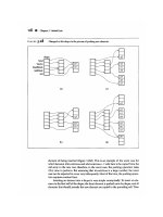
We show an example output from a run of the Duck, Duck, Goose program in
Figure 3.20.
Figure 3.20: Sample output from the Duck, Duck,
Goose program.

Note that each iteration in this particular execution of this program produces a
different outcome, due to the different initial configurations and the use of
random choices to identify ducks and geese. Likewise, whether the "Duck" or the
"Goose" wins the race is also different, depending on random choices. This
execution shows a situation where the next child after the "it" person is
immediately identified as the "Goose," as well a situation where the "it" person
walks all the way around the group of children before identifying the "Goose."
Such situations also illustrate the usefulness of using a circularly linked list to
simulate circular games like Duck, Duck, Goose.
3.4.2 Sorting a Linked List

186
We show in Code Fragment 3.27 theinsertion-sort algorithm (Section 3.1.2) for a
doubly linked list. A Java implementation is given in Code Fragment 3.28.
Code Fragment 3.27: High-level pseudo-code
description of insertion-sort on a doubly linked list.

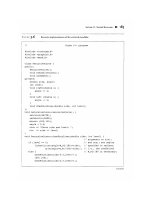
Code Fragment 3.28: Java implementation of the
insertion-sort algorithm on a doubly linked list
represented by class DList (see Code Fragments 3.22
–
3.24
).

187

3.5 Recursion
We have seen that repetition can be achieved by writing loops, such as for loops and
while loops. Another way to achieve repetition is through recursion, which occurs
when a function calls itself. We have seen examples of methods calling other
methods, so it should come as no surprise that most modern programming languages,
including Java, allow a method to call itself. In this section, we will see why this
capability provides an elegant and powerful alternative for performing repetitive
tasks.
The Factorial function
To illustrate recursion, let us begin with a simple example of computing the value
of the factorial function. The factorial of a positive integer n, denoted n!, is defined
as the product of the integers from 1 to n. If n = 0, then n! is defined as 1 by
convention. More formally, for any integer n ≥ 0,

For example, 5! = 5·4·3·2·1 = 120. To make the connection with methods clearer,
we use the notation factorial(n) to denote n!.

188
The factorial function can be defined in a manner that suggests a recursive
formulation. To see this, observe that
factorial(5) = 5 · (4 · 3 · 2 · 1) = 5 · factorial(4).
Thus, we can define factorial(5) in terms of factorial(4). In general, for a
positive integer n, we can define factorial(n) to be n·factorial(n − 1). This
leads to the following recursive definition.

This definition is typical of many recursive definitions. First, it contains one or
more base cases, which are defined nonrecursively in terms of fixed quantities. In
this case, n = 0 is the base case. It also contains one or more recursive cases, which
are defined by appealing to the definition of the function being defined. Observe
that there is no circularity in this definition, because each time the function is

invoked, its argument is smaller by one.
A Recursive Implementation of the Factorial Function
Let us consider a Java implementation of the factorial function shown in Code
Fragment 3.29 under the name recursiveFactorial(). Notice that no
looping was needed here. The repeated recursive invocations of the function takes
the place of looping.
Code Fragment 3.29: A recursive implementation of
the factorial function.

We can illustrate the execution of a recursive function definition by means of a
recursion trace. Each entry of the trace corresponds to a recursive call. Each new
recursive function call is indicated by an arrow to the newly called function. When
the function returns, an arrow showing this return is drawn and the return value may
be indicated with this arrow. An example of a trace is shown in Figure 3.21.
What is the advantage of using recursion? Although the recursive implementation
of the factorial function is somewhat simpler than the iterative version, in this case
there is no compelling reason for preferring recursion over iteration. For some

189
problems, however, a recursive implementation can be significantly simpler and
easier to understand than an iterative implementation. Such an example follows.
Figure 3.21: A recursion trace for the call
recursiveFactorial(4).

Drawing an English Ruler
As a more complex example of the use of recursion, consider how to draw the
markings of a typical English ruler. A ruler is broken up into 1-inch intervals, and
each interval consists of a set of ticks placed at intervals of 1/2 inch, 1/4 inch, and
so on. As the size of the interval decreases by half, the tick length decreases by one.
(See Figure 3.22

.)
Figure 3.22: Three sample outputs of the ruler-
drawing function: (a) a 2-inch ruler with major tick
length 4; (b) a 1-inch ruler with major tick length 5; (c) a
3-inch ruler with major tick length 3.

190

Each multiple of 1 inch also has a numeric label. The longest tick length is called
the major tick length. We will not worry about actual distances, however, and just
print one tick per line.
A Recursive Approach to Ruler Drawing
Our approach to drawing such a ruler consists of three functions. The main function
drawRuler() draws the entire ruler. Its arguments are the total number of inches
in the ruler, nInches, and the major tick length, majorLength. The utility
function drawOneTick() draws a single tick of the given length. It can also be
given an optional integer label, which is printed if it is nonnegative.
The interesting work is done by the recursive function drawTicks(), which
draws the sequence of ticks within some interval. Its only argument is the tick
length associated with the interval's central tick. Consider the 1-inch ruler with
major tick length 5 shown in Figure 3.22(b)
. Ignoring the lines containing 0 and 1,
let us consider how to draw the sequence of ticks lying between these lines. The
central tick (at 1/2 inch) has length 4. Observe that the two patterns of ticks above
and below this central tick are identical, and each has a central tick of length 3. In
general, an interval with a central tick length L ≥ 1 is composed of the following:
• An interval with a central tick length L − 1

191
• A single tick of length L

• A interval with a central tick length L − 1.
With each recursive call, the length decreases by one. When the length drops to
zero, we simply return. As a result, this recursive process will always terminate.
This suggests a recursive process, in which the first and last steps are performed by
calling the drawTicks(L − 1) recursively. The middle step is performed by
calling the function drawOneTick(L). This recursive formulation is shown in
Code Fragment 3.30. As in the factorial example, the code has a base case (when L
= 0). In this instance we make two recursive calls to the function.
Code Fragment 3.30: A recursive implementation of
a function that draws a ruler.

Illustrating Ruler Drawing using a Recursion Trace
The recursive execution of the recursive drawTicks function, defined above, can
be visualized using a recursion trace.

192
The trace for drawTicks is more complicated than in the factorial example,
however, because each instance makes two recursive calls. To illustrate this, we
will show the recursion trace in a form that is reminiscent of an outline for a
document. See Figure 3.23.
Figure 3.23: A partial recursion trace for the call
drawTicks(3). The second pattern of calls for
drawTicks(2) is not shown, but it is identical to the
first.

Throughout this book we shall see many other examples of how recursion can be
used in the design of data structures and algorithms.

193
Further Illustrations of Recursion

As we discussed above, recursion is the concept of defining a method that makes a
call to itself. Whenever a method calls itself, we refer to this as a recursive call. We
also consider a method M to be recursive if it calls another method that ultimately
leads to a call back to M.
The main benefit of a recursive approach to algorithm design is that it allows us to
take advantage of the repetitive structure present in many problems. By making our
algorithm description exploit this repetitive structure in a recursive way, we can
often avoid complex case analyses and nested loops. This approach can lead to
more readable algorithm descriptions, while still being quite efficient.
In addition, recursion is a useful way for defining objects that have a repeated
similar structural form, such as in the following examples.
Example 3.1: Modern operating systems define file-system directories (which
are also sometimes called "folders") in a recursive way. Namely, a file system
consists of a top-level directory, and the contents of this directory consists of files
and other directories, which in turn can contain files and other directories, and so
on. The base directories in the file system contain only files, but by using this
recursive definition, the operating system allows for directories to be nested
arbitrarily deep (as long as there is enough space in memory).
Example 3.2: Much of the syntax in modern programming languages is defined
in a recursive way. For example, we can define an argument list in Java using the
following notation:
argument-list:
argument
argument-list, argument
In other words, an argument list consists of either (i) an argument or (ii) an
argument list followed by a comma and an argument. That is, an argument list
consists of a comma-separated list of arguments. Similarly, arithmetic expressions
can be defined recursively in terms of primitives (like variables and constants) and
arithmetic expressions.
Example 3.3: There are many examples of recursion in art and nature. One of

the most classic examples of recursion used in art is in the Russian Matryoshka
dolls. Each doll is made of solid wood or is hollow and contains another
Matryoshka doll inside it.
3.5.1 Linear Recursion

194
The simplest form of recursion is linear recursion, where a method is defined so
that it makes at most one recursive call each time it is invoked. This type of
recursion is useful when we view an algorithmic problem in terms of a first or last
element plus a remaining set that has the same structure as the original set.
Summing the Elements of an Array Recursively
Suppose, for example, we are given an array, A, of n integers that we wish to sum
together. We can solve this summation problem using linear recursion by
observing that the sum of all n integers in A is equal to A[0], if n = 1, or the sum
of the first n − 1 integers in A plus the last element in A. In particular, we can
solve this summation problem using the recursive algorithm described in Code
Fragment 3.31.
Code Fragment 3.31: Summing the elements in an
array using linear recursion.

This example also illustrates an important property that a recursive method should
always possess—the method terminates. We ensure this by writing a nonrecursive
statement for the case n = 1. In addition, we always perform the recursive call on
a smaller value of the parameter (n − 1) than that which we are given (n), so that,
at some point (at the "bottom" of the recursion), we will perform the nonrecursive
part of the computation (returning A[0]). In general, an algorithm that uses linear
recursion typically has the following form:
• Test for base cases. We begin by testing for a set of base cases (there
should be at least one). These base cases should be defined so that every
possible chain of recursive calls will eventually reach a base case, and the

handling of each base case should not use recursion.
• Recur. After testing for base cases, we then perform a single recursive
call. This recursive step may involve a test that decides which of several
possible recursive calls to make, but it should ultimately choose to make just
one of these calls each time we perform this step. Moreover, we should define
each possible recursive call so that it makes progress towards a base case.

195
Analyzing Recursive Algorithms using Recursion Traces
We can analyze a recursive algorithm by using a visual tool known as a recursion
trace. We used recursion traces, for example, to analyze and visualize the
recursive Fibonacci function of Section 3.5
, and we will similarly use recursion
traces for the recursive sorting algorithms of Sections 11.1
and 11.2.
To draw a recursion trace, we create a box for each instance of the method and
label it with the parameters of the method. Also, we visualize a recursive call by
drawing an arrow from the box of the calling method to the box of the called
method. For example, we illustrate the recursion trace of the LinearSum
algorithm of Code Fragment 3.31 in Figure 3.24. We label each box in this trace
with the parameters used to make this call. Each time we make a recursive call,
we draw a line to the box representing the recursive call. We can also use this
diagram to visualize stepping through the algorithm, since it proceeds by going
from the call for n to the call for n − 1, to the call for n − 2, and so on, all the way
down to the call for 1. When the final call finishes, it returns its value back to the
call for 2, which adds in its value, and returns this partial sum to the call for 3, and
so on, until the call for n − 1 returns its partial sum to the call for n.
Figure 3.24: Recursion trace for an execution of
LinearSum(A,n) with input parameters A = {4,3,6,2,5}
and n = 5.

From Figure 3.24, it should be clear that for an input array of size n, Algorithm
LinearSum makes n calls. Hence, it will take an amount of time that is roughly
proportional to n, since it spends a constant amount of time performing the

196
nonrecursive part of each call. Moreover, we can also see that the memory space
used by the algorithm (in addition to the array A) is also roughly proportional to n,
since we need a constant amount of memory space for each of the n boxes in the
trace at the time we make the final recursive call (for n = 1).
Reversing an Array by Recursion
Next, let us consider the problem of reversing the n elements of an array, A, so
that the first element becomes the last, the second element becomes second to the
last, and so on. We can solve this problem using linear recursion, by observing
that the reversal of an array can be achieved by swapping the first and last
elements and then recursively reversing the remaining elements in the array. We
describe the details of this algorithm in Code Fragment 3.32, using the convention
that the first time we call this algorithm we do so as ReverseArray(A,0,n − 1).
Code Fragment 3.32: Reversing the elements of an
array using linear recursion.

Note that, in this algorithm, we actually have two base cases, namely, when i = j
and when i > j. Moreover, in either case, we simply terminate the algorithm, since
a sequence with zero elements or one element is trivially equal to its reversal.
Furthermore, note that in the recursive step we are guaranteed to make progress
towards one of these two base cases. If n is odd, we will eventually reach the i = j
case, and if n is even, we will eventually reach the i > j case. The above argument
immediately implies that the recursive algorithm of Code Fragment 3.32 is
guaranteed to terminate.
Defining Problems in Ways That Facilitate Recursion

To design a recursive algorithm for a given problem, it is useful to think of the
different ways we can subdivide this problem to define problems that have the
same general structure as the original problem. This process sometimes means we
need to redefine the original problem to facilitate similar-looking subproblems.
For example, with the ReverseArray algorithm, we added the parameters i and
j so that a recursive call to reverse the inner part of the array A would have the
same structure (and same syntax) as the call to reverse all of A. Then, rather than

197
initially calling the algorithm as ReverseArray(A), we call it initially as
ReverseArray(A,0,n−1). In general, if one has difficulty finding the repetitive
structure needed to design a recursive algorithm, it is sometimes useful to work
out the problem on a few concrete examples to see how the subproblems should
be defined.
Tail Recursion
Using recursion can often be a useful tool for designing algorithms that have
elegant, short definitions. But this usefulness does come at a modest cost. When
we use a recursive algorithm to solve a problem, we have to use some of the
memory locations in our computer to keep track of the state of each active
recursive call. When computer memory is at a premium, then, it is useful in some
cases to be able to derive nonrecursive algorithms from recursive ones.
We can use the stack data structure, discussed in Section 5.1, to convert a
recursive algorithm into a nonrecursive algorithm, but there are some instances
when we can do this conversion more easily and efficiently. Specifically, we can
easily convert algorithms that use tail recursion. An algorithm uses tail recursion
if it uses linear recursion and the algorithm makes a recursive call as its very last
operation. For example, the algorithm of Code Fragment 3.32 uses tail recursion
to reverse the elements of an array.
It is not enough that the last statement in the method definition include a recursive
call, however. In order for a method to use tail recursion, the recursive call must

be absolutely the last thing the method does (unless we are in a base case, of
course). For example, the algorithm of Code Fragment 3.31 does not use tail
recursion, even though its last statement includes a recursive call. This recursive
call is not actually the last thing the method does. After it receives the value
returned from the recursive call, it adds this value to A [n − 1] and returns this
sum. That is, the last thing this algorithm does is an add, not a recursive call.
When an algorithm uses tail recursion, we can convert the recursive algorithm
into a nonrecursive one, by iterating through the recursive calls rather than calling
them explicitly. We illustrate this type of conversion by revisiting the problem of
reversing the elements of an array. In Code Fragment 3.33
, we give a
nonrecursive algorithm that performs this task by iterating through the recursive
calls of the algorithm of Code Fragment 3.32.
We initially call this algorithm as
IterativeReverseArray (A, 0,n − 1).
Code Fragment 3.33: Reversing the elements of an
array using iteration.

198

3.5.2 Binary Recursion
When an algorithm makes two recursive calls, we say that it uses binary recursion.
These calls can, for example, be used to solve two similar halves of some problem,
as we did in Section 3.5 for drawing an English ruler. As another application of
binary recursion, let us revisit the problem of summing the n elements of an integer
array A. In this case, we can sum the elements in A by: (i) recursively summing the
elements in the first half of A; (ii) recursively summing the elements in the second
half of A; and (iii) adding these two values together. We give the details in the
algorithm of Code Fragment 3.34, which we initially call as BinarySum(A,0,n).
Code Fragment 3.34: Summing the elements in an

array using binary recursion.

To analyze Algorithm BinarySum, we consider, for simplicity, the case where n
is a power of two. The general case of arbitrary n is considered in Exercise R-4.4.
Figure 3.25 shows the recursion trace of an execution of method BinarySum(0,8).
We label each box with the values of parameters i and n, which represent the
starting index and length of the sequence of elements to be reversed, respectively.
Notice that the arrows in the trace go from a box labeled (i,n) to another box labeled
(i,n/2) or (i + n/2,n/2). That is, the value of parameter n is halved at each recursive
call. Thus, the depth of the recursion, that is, the maximum number of method
instances that are active at the same time, is 1 + log
2
n. Thus, Algorithm
BinarySum uses an amount of additional space roughly proportional to this value.
This is a big improvement over the space needed by the LinearSum method of Code
Fragment 3.31. The running time of Algorithm BinarySum is still roughly

199
proportional to n, however, since each box is visited in constant time when stepping
through our algorithm and there are 2n − 1 boxes.
Figure 3.25: Recursion trace for the execution of
BinarySum(0,8).

Computing Fibonacci Numbers via Binary Recursion
Let us consider the problem of computing the kth Fibonacci number. Recall from
Section 2.2.3, that the Fibonacci numbers are recursively defined as follows:
F
0
= 0
F

1
= 1
F
i
= F
i−1
+ F
i−2
for i < 1.
By directly applying this definition, Algorithm BinaryFib, shown in Code
Fragment 3.35, computes the sequence of Fibonacci numbers using binary
recursion.
Code Fragment 3.35: Computing the kth Fibonacci
number using binary recursion.


200
Unfortunately, in spite of the Fibonacci definition looking like a binary recursion,
using this technique is inefficient in this case. In fact, it takes an exponential
number of calls to compute the kth Fibonacci number in this way. Specifically, let
n
k
denote the number of calls performed in the execution of BinaryFib(k).
Then, we have the following values for the n
k
's:
n
0
= 1
n

1
= 1
n
2
= n
1
+ n
0
+ 1 = 1 + 1 + 1 = 3
n
3
= n
2
+ n
1
+ 1 = 3 + 1 + 1 = 5
n
4
= n
3
+ n2 + 1 = 5 + 3 + 1 = 9
n
5
= n
4
+ n
3
+ 1 = 9 + 5 + 1 = 15
n
6

= n
5
+ n
4
+ 1 = 15 + 9 + 1 = 25
n
7
= n
6
+ n
5
+ 1 = 25 + 15 + 1 = 41
n
8
= n
7
+ n
6
+ 1 = 41 + 25 + 1 = 67.
If we follow the pattern forward, we see that the number of calls more than
doubles for each two consecutive indices. That is, n
4
is more than twice n
2
n
5
is
more than twice n
3
, n

6
is more than twice n
4
, and so on. Thus, n
k
> 2
k/2
, which
means that BinaryFib(k) makes a number of calls that are exponential in k. In
other words, using binary recursion to compute Fibonacci numbers is very
inefficient.
Computing Fibonacci Numbers via Linear Recursion
The main problem with the approach above, based on binary recursion, is that the
computation of Fibonacci numbers is really a linearly recursive problem. It is not
a good candidate for using binary recursion. We simply got tempted into using
binary recursion because of the way the kth Fibonacci number, F
k
, depends on the
two previous values, F
k−1
and F
k−2
. But we can compute F
k
much more efficiently
using linear recursion.
In order to use linear recursion, however, we need to slightly redefine the
problem. One way to accomplish this conversion is to define a recursive function
that computes a pair of consecutive Fibonacci numbers (F
k

,F
k
−1) using the
convention F−1 = 0. Then we can use the linearly recursive algorithm shown in
Code Fragment 3.36.


201
Code Fragment 3.36: Computing the kth Fibonacci
number using linear recursion.

The algorithm given in Code Fragment 3.36 shows that using linear recursion to
compute Fibonacci numbers is much more efficient than using binary recursion.
Since each recursive call to LinearFibonacci decreases the argument k by 1,
the original call LinearFibonacci(k) results in a series of k − 1 additional
calls. That is, computing the kth Fibonacci number via linear recursion requires k
method calls. This performance is significantly faster than the exponential time
needed by the algorithm based on binary recursion, which was given in Code
Fragment 3.35. Therefore, when using binary recursion, we should first try to
fully partition the problem in two (as we did for summing the elements of an
array) or, we should be sure that overlapping recursive calls are really necessary.
Usually, we can eliminate overlapping recursive calls by using more memory to
keep track of previous values. In fact, this approach is a central part of a technique
called dynamic programming, which is related to recursion and is discussed in
Section 12.5.2.
3.5.3 Multiple Recursion
Generalizing from binary recursion, we use multiple recursion when a method may
make multiple recursive calls, with that number potentially being more than two.
One of the most common applications of this type of recursion is used when we
wish to enumerate various configurations in order to solve a combinatorial puzzle.

For example, the following are all instances of summation puzzles:
pot + pan = bib
dog + cat = pig
boy + girl = baby

202
To solve such a puzzle, we need to assign a unique digit (that is, 0,1,…, 9) to each
letter in the equation, in order to make the equation true. Typically, we solve such a
puzzle by using our human observations of the particular puzzle we are trying to
solve to eliminate configurations (that is, possible partial assignments of digits to
letters) until we can work though the feasible configurations left, testing for the
correctness of each one.
If the number of possible configurations is not too large, however, we can use a
computer to simply enumerate all the possibilities and test each one, without
employing any human observations. In addition, such an algorithm can use multiple
recursion to work through the configurations in a systematic way. We show
pseudocode for such an algorithm in Code Fragment 3.37. To keep the description
general enough to be used with other puzzles, the algorithm enumerates and tests all
k-length sequences without repetitions of the elements of a given set U. We build
the sequences of k elements by the following steps:
1. Recursively generating the sequences of k − 1 elements
2. Appending to each such sequence an element not already contained in it.
Throughout the execution of the algorithm, we use the set U to keep track of the
elements not contained in the current sequence, so that an element e has not been
used yet if and only if e is in U.
Another way to look at the algorithm of Code Fragment 3.37 is that it enumerates
every possible size-k ordered subset of U, and tests each subset for being a possible
solution to our puzzle.
For summation puzzles, U = {0,1,2,3,4,5,6,7,8,9} and each position in the sequence
corresponds to a given letter. For example, the first position could stand for b, the

second for o, the third for y, and so on.
Code Fragment 3.37: Solving a combinatorial puzzle
by enumerating and testing all possible configurations.

203

In Figure 3.26, we show a recursion trace of a call to PuzzleSolve(3,S,U),
where S is empty and U = {a,b,c}. During the execution, all the permutations of the
three characters are generated and tested. Note that the initial call makes three
recursive calls, each of which in turn makes two more. If we had executed
PuzzleSolve(3,S, U) on a set U consisting of four elements, the initial call
would have made four recursive calls, each of which would have a trace looking
like the one in Figure 3.26.
Figure 3.26: Recursion trace for an execution of
PuzzleSolve(3,S,U), where S is empty and U = {a, b,
c}. This execution generates and tests all permutations
of a, b, and c. We show the permutations generated
directly below their respective boxes.


204
3.6 Exercises
For source code and help with exercises, please visit
java.datastructures.net
.
Reinforcement
R-3.1
The add and remove methods of Code Fragments 3.3 and 3.4 do not keep
track of the number,n, of non-null entries in the array, a. Instead, the unused
cells point to the null object. Show how to change these methods so that they

keep track of the actual size of a in an instance variable n.
R-3.2
Describe a way to use recursion to add all the elements in a n × n (two
dimensional) array of integers.
R-3.3
Explain how to modify the Caesar cipher program (Code Fragment 3.9) so that
it performs ROT 13 encryption and decryption, which uses 13 as the alphabet
shift amount. How can you further simplify the code so that the body of the
decrypt method is only a single line?
R-3.4
Explain the changes that would have be made to the program of Code Fragment
3.9 so that it could perform the Caesar cipher for messages that are written in an
alphabet-based language other than English, such as Greek, Russian, or Hebrew.
R-3.5
What is the exception that is thrown when advance or remove is called on an
empty list, from Code Fragment 3.25? Explain how to modify these methods so
that they give a more instructive exception name for this condition.
R-3.6
Give a recursive definition of a singly linked list.
R-3.7
Describe a method for inserting an element at the beginning of a singly linked
list. Assume that the list does not have a sentinel header node, and instead uses
a variable head to reference the first node in the list.

205
R-3.8
Give an algorithm for finding the penultimate node in a singly linked list where
the last element is indicated by a null next reference.
R-3.9
Describe a nonrecursive method for finding, by link hopping, the middle node

of a doubly linked list with header and trailer sentinels. (Note: This method
must only use link hopping; it cannot use a counter.) What is the running time
of this method?
R-3.10
Describe a recursive algorithm for finding the maximum element in an array A
of n elements. What is your running time and space usage?
R-3.11
Draw the recursion trace for the execution of method ReverseArray (A ,0,4)
(Code Fragment 3.32) on array A = {4,3,6,2,5}.
R-3.12
Draw the recursion trace for the execution of method PuzzleSolve(3,S, U)
(Code Fragment 3.37), where S is empty and U = {a,b,c,d}.
R-3.13
Write a short Java method that repeatedly selects and removes a random entry
from an array until the array holds no more entries.
R-3.14
Write a short Java method to count the number of nodes in a circularly linked
list.
Creativity
C-3.1
Give Java code for performing add(e) and remove(i) methods for game
entries, stored in an array a, as in Code Fragments 3.3 and 3.4, except now don't
maintain the game entries in order. Assume that we still need to keep n entries
stored in indices 0 to n − 1. Try to implement the add and remove methods
without using any loops, so that the number of steps they perform does not
depend on n.

206
C-3.2
Let A be an array of size n ≥ 2 containing integers from 1 to n − 1, inclusive,

with exactly one repeated. Describe a fast algorithm for finding the integer in A
that is repeated.
C-3.3
Let B be an array of size n ≥ 6 containing integers from 1 to n − 5, inclusive,
with exactly five repeated. Describe a good algorithm for finding the five
integers in B that are repeated.
C-3.4
Suppose you are designing a multi-player game that has n ≥ 1000 players,
numbered 1 to n, interacting in an enchanted forest. The winner of this game is
the first player who can meet all the other players at least once (ties are
allowed). Assuming that there is a method meet(i,j), which is called each time a
player i meets a player j (with i ≠ j), describe a way to keep track of the pairs of
meeting players and who is the winner.
C-3.5
Give a recursive algorithm to compute the product of two positive integers, m
and n, using only addition and subtraction.
C-3.6
Describe a fast recursive algorithm for reversing a singly linked list L, so that
the ordering of the nodes becomes opposite of what it was before, a list has only
one position, then we are done; the list is already reversed. Otherwise, remove
C-3.7
Describe a good algorithm for concatenating two singly linked lists L and M,
with header sentinels, into a single list L ′ that contains all the nodes of L
followed by all the nodes of M.
C-3.8
Give a fast algorithm for concatenating two doubly linked lists L and M, with
header and trailer sentinel nodes, into a single list L ′.
C-3.9
Describe in detail how to swap two nodes x and y in a singly linked list L given
references only to x and y. Repeat this exercise for the case when L is a doubly

linked list. Which algorithm takes more time?

207
C-3.10
Describe in detail an algorithm for reversing a singly linked list L using only a
constant amount of additional space and not using any recursion.
C-3.11
In the Towers of Hanoi puzzle, we are given a platform with three pegs, a, b,
and c, sticking out of it. On peg a is a stack of n disks, each larger than the next,
so that the smallest is on the top and the largest is on the bottom. The puzzle is
to move all the disks from peg a to peg c, moving one disk at a time, so that we
never place a larger disk on top of a smaller one. See Figure 3.27
for an
example of the case n = 4. Describe a recursive algorithm for solving the
Towers of Hanoi puzzle for arbitrary n. (Hint: Consider first the subproblem of
moving all but the nth disk from peg a to another peg using the third as
"temporary storage." )
Figure 3.27: An illustration of the Towers of Hanoi
puzzle.

C-3.12
Describe a recursive method for converting a string of digits into the integer it
represents. For example, "13531" represents the integer 13,531.
C-3.13
Describe a recursive algorithm that counts the number of nodes in a singly
linked list.
C-3.14

208
Write a recursive Java program that will output all the subsets of a set of n

elements (without repeating any subsets).
C-3.15
Write a short recursive Java method that finds the minimum and maximum
values in an array of int values without using any loops.
C-3.16
Describe a recursive algorithm that will check if an array A of integers contains
an integer A[i] that is the sum of two integers that appear earlier in A, that is,
such that A[i] = A[j] +A[k] for j,k > i.
C-3.17
Write a short recursive Java method that will rearrange an array of int values
so that all the even values appear before all the odd values.
C-3.18
Write a short recursive Java method that takes a character string s and outputs
its reverse. So for example, the reverse of "pots&pans" would be
"snap&stop".
C-3.19
Write a short recursive Java method that determines if a string s is a palindrome,
that is, it is equal to its reverse. For example, "racecar" and
"gohangasalamiimalasagnahog" are palindromes.
C-3.20
Use recursion to write a Java method for determining if a string s has more
vowels than consonants.
C-3.21
Suppose you are given two circularly linked lists, L and M, that is, two lists of
nodes such that each node has a nonnull next node. Describe a fast algorithm for
telling if L and M are really the same list of nodes, but with different (cursor)
starting points.
C-3.22
Given a circularly linked list L containing an even number of nodes, describe
how to split L into two circularly linked lists of half the size.

209
Projects
P-3.1
Write a Java program for a matrix class that can add and multiply arbitrary two-
dimensional arrays of integers.
P-3.2
Perform the previous project, but use generic types so that the matrices involved
can contain arbitrary number types.
P-3.3
Write a class that maintains the top 10 scores for a game application,
implementing the add and remove methods of Section 3.1.1, but using a
singly linked list instead of an array.
P-3.4
Perform the previous project, but use a doubly linked list. Moreover, your
implementation of remove(i) should make the fewest number of pointer hops
to get to the game entry at index i.
P-3.5
Perform the previous project, but use a linked list that is both circularly linked
and doubly linked.
P-3.6
Write a program for solving summation puzzles by enumerating and testing all
possible configurations. Using your program, solve the three puzzles given in
Section 3.5.3.

P-3.7
Write a program that can perform encryption and decryption using an arbitrary
substitution cipher. In this case, the encryption array is a random shuffling of
the letters in the alphabet. Your program should generate a random encryption
array, its corresponding decryption array, and use these to encode and decode a

message.
P-3.8
Write a program that can perform the Caesar cipher for English messages that
include both upper and lowercase characters.

210