Data Structures and Algorithms in Java 4th phần 7 pptx

• If k = e.getKey(), then we have found the entry we were looking for,
and the search terminates successfully returning e.
• If k < e.getKey(), then we recur on the first half of the array list, that is,
on the range of indices from low to mid − 1.
• If k > e.getKey(), we recur on the range of indices from mid + 1 to
high.
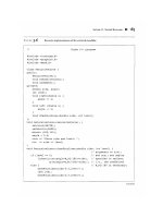
This search method is called binary search, and is given in pseudo-code in Code
Fragment 9.9. Operation find(k) on an n-entry dictionary implemented with an
ordered array list S consists of calling BinarySearch(S,k,0,n − 1).
Code Fragment 9.9: Binary search in an ordered
array list.

We illustrate the binary search algorithm in Figure 9.8.
Figure 9.8: Example of a binary search to perform
operation find(22), in a dictio nary with integer
keys, implemented with an ordered array list. For
simplicity, we show the keys stored in the dictionary
but not the whole entries.

554

Considering the running time of binary search, we observe that a constant num
ber of primitive operations are executed at each recursive call of method Binary
Search. Hence, the running time is proportional to the number of recursive calls
performed. A crucial fact is that with each recursive call the number of candidate
entries still to be searched in the array list S is given by the value
high − low + 1.
Moreover, the number of remaining candidates is reduced by at least one half with
each recursive call. Specifically, from the definition of mid, the number of remain
ing candidates is either

or

Initially, the number of candidate entries is n; after the first call to
BinarySearch, it is at most n/2; after the second call, it is at most n/4; and so
on. In general, after the ith call to BinarySearch, the number of candidate
entries remaining is at most n/2
i
. In the worst case (unsuccessful search), the
recursive calls stop when there are no more candidate entries. Hence, the
maximum number of recursive calls performed, is the smallest integer m such that
n/2
m
< 1.

555
In other words (recalling that we omit a logarithm's base when it is 2), m > logn.
Thus, we have
m = logn + 1,
which implies that binary search runs in O(logn) time.
There is a simple variation of binary search that performs findAll(k) in time
O(logn + s), where s is the number of entries in the iterator returned. The details
are left as an exercise (C-9.4).
Thus, we can use an ordered search table to perform fast dictionary searches, but
using such a table for lots of dictionary updates would take a considerable amount
of time. For this reason, the primary applications for search tables are in situations
where we expect few updates to the dictionary but many searches. Such a
situation could arise, for example, in an ordered list of English words we use to
order entries in an encyclopedia or help file.
Comparing Dictionary Implementations
Table 9.3 compares the running times of the methods of a dictionary realized by

either an unordered list, a hash table, or an ordered search table. Note that an
unordered list allows for fast insertions but slow searches and removals, whereas
a search table allows for fast searches but slow insertions and removals.
Incidentally, although we don't explicitly discuss it, we note that a sorted list
implemented with a doubly linked list would be slow in performing almost all the
dictionary operations. (See Exercise R-9.3.)
Table 9.3: Comparison of the running times of the
methods of a dictionary realized by means of an
unordered list, a hash table, or an ordered search
table. We let n denote the number of entries in the
dictionary, N denote the capacity of the bucket array
in the hash table implementations, and s denote the
size of collection returned by operation findAll. The
space requirement of all the implementations is O(n),
assuming that the arrays supporting the hash table
and search table implementations are maintained such
that their capacity is proportional to the number of
entries in the dictionary.

556
Method
List
Hash Table
Search Table
size, isEmpty
O(1)
O(1)
O(1)
entries
O(n)

O(n)
O(n)
find
O(n)
O(1) exp., O(n) worst-case
O(logn)
findAll
O(n)
O(1 + s) exp., O(n) worst-case
O(logn + s)
insert
O(1)
O(1)
O(n)
remove

557
O(n)
O(1) exp., O(n) worst-case
O(n)
9.4 Skip Lists
An interesting data structure for efficiently realizing the dictionary ADT is the skip
list. This data structure makes random choices in arranging the entries in such a way
that search and update times are O(logn) on average, where n is the number of entries
in the dictionary. Interestingly, the notion of average time complexity used here does
not depend on the probability distribution of the keys in the input. Instead, it depends
on the use of a random-number generator in the implementation of the insertions to
help decide where to place the new entry. The running time is averaged over all
possible outcomes of the random numbers used when inserting entries.
Because they are used extensively in computer games, cryptography, and computer

simulations, methods that generate numbers that can be viewed as random numbers
are built into most modern computers. Some methods, called pseudorandom number
generators, generate random-like numbers deterministically, starting with an initial
number called a seed. Other methods use hardware devices to extract "true" random
numbers from nature. In any case, we will assume that our computer has access to
numbers that are sufficiently random for our analysis.
The main advantage of using randomization in data structure and algorithm design is
that the structures and methods that result are usually simple and efficient. We can
devise a simple randomized data structure, called the skip list, which has the same
logarithmic time bounds for searching as is achieved by the binary searching
algorithm. Nevertheless, the bounds are expected for the skip list, while they are
worst-case bounds for binary searching in a look-up table. On the other hand, skip
lists are much faster than look-up tables for dictionary updates.
A skip list S for dictionary D consists of a series of lists {S
0
, S
1
, , S
h
}. Each list S
i

stores a subset of the entries of D sorted by a nondecreasing key plus entries with two
special keys, denoted −∞ and +∞, where −∞ is smaller than every possible key that
can be inserted in D and +∞ is larger than every possible key that can be inserted in
D. In addition, the lists in S satisfy the following:
• List S
0
contains every entry of dictionary D (plus the special entries with keys −∞
and +∞).

• For i = 1, , h − 1, list S
i
contains (in addition to −∞ and +∞) a randomly
generated subset of the entries in list S
i−1
.
• List S
h
contains only −∞ and +∞.

558
An example of a skip list is shown in Figure 9.9. It is customary to visualize a skip
list S with list S
0
at the bottom and lists S
1
,…,S
h
above it. Also, we refer to h as the
height of skip list S.
Figure 9.9: Example of a skip list storing 10 entries.
For simplicity, we show only the keys of the entries.

Intuitively, the lists are set up so that S
i+1
contains more or less every other entry in
S
i
. As we shall see in the details of the insertion method, the entries in S
i+1

are chosen
at random from the entries in S

th
i
by picking each entry from S
i
to also be in S
i+1
wi
probability 1/2. That is, in essence, we "flip a coin" for each entry in S
i
and place that
entry in S
i+1
if the coin comes up "heads." Thus, we expect S
1
to have about n/2
entries, S
2
to have about n/4 entries, and, in general, S
i
to have about n/2
i
entries. In
other words, we expect the height h of S to be about logn. The halving of the number
of entries from one list to the next is not enforced as an explicit property of skip lists,
however. Instead, randomization is used.
Using the position abstraction used for lists and trees, we view a skip list as a two-
dimensional collection of positions arranged horizontally into levels and vertically

into towers. Each level is a list S
i
and each tower contains positions storing the same
entry across consecutive lists. The positions in a skip list can be traversed using the
following operations:
next(p): Return the position following p on the same level.
prev(p): Return the position preceding p on the same level.
below(p): Return the position below p in the same tower.
above(p): Return the position above p in the same tower.
We conventionally assume that the above operations return a null position if the
position requested does not exist. Without going into the details, we note that we can
easily implement a skip list by means of a linked structure such that the above
traversal methods each take O(1) time, given a skip-list position p. Such a linked

559
structure is essentially a collection of h doubly linked lists aligned at towers, which
are also doubly linked lists.
9.4.1 Search and Update Operations in a Skip List
The skip list structure allows for simple dictionary search and update algorithms. In
fact, all of the skip list search and update algorithms are based on an elegant
SkipSearch method that takes a key k and finds the position p of the entry e in
list S
0
such that e has the largest key (which is possibly −∞) less than or equal to k.
Searching in a Skip List
Suppose we are given a search key k. We begin the SkipSearch method by
setting a position variable p to the top-most, left position in the skip list S, called
the start position of S. That is, the start position is the position of S
h
storing the

special entry with key −∞. We then perform the following steps (see Figure 9.10),
where key(p) denotes the key of the entry at position p:
1. If S.below(p) is null, then the search terminates—we are at the bottom
and have located the largest entry in S with key less than or equal to the search
key k. Otherwise, we drop down to the next lower level in the present tower by
setting p ← S.below(p).
2. Starting at position p, we move p forward until it is at the right-most
position on the present level such that key(p) ≤ k. We call this the scan forward
step. Note that such a position always exists, since each level contains the keys
+∞ and −∞. In fact, after we perform the scan forward for this level, p may
remain where it started. In any case, we then repeat the previous step.
Figure 9.10: Example of a search in a skip list. The
positions visited when searching for key 50 are
highlighted in blue.


560
We give a pseudo-code description of the skip-list search algorithm,
SkipSearch, in Code Fragment 9.10. Given this method, it is now easy to
implement the operation find(k)we simply perform p ← SkipSearch(k) and
test whether or not key(p) = k. If these two keys are equal, we return p;
otherwise, we return null.
Code Fragment 9.10: Search in a skip list S. Variable
s holds the start position of S.

As it turns out, the expected running time of algorithm SkipSearch on a skip
list with n entries is O(logn). We postpone the justification of this fact, however,
until after we discuss the implementation of the update methods for skip lists.
Insertion in a Skip List
The insertion algorithm for skip lists uses randomization to decide the height of

the tower for the new entry. We begin the insertion of a new entry (k,v) by
performing a SkipSearch(k) operation. This gives us the position p of the
bottom-level entry with the largest key less than or equal to k (note that p may
hold the special entry with key −∞). We then insert (k, v) immediately after
position p. After inserting the new entry at the bottom level, we "flip" a coin. If
the flip comes up tails, then we stop here. Else (the flip comes up heads), we
backtrack to the previous (next higher) level and insert (k,v) in this level at the
appropriate position. We again flip a coin; if it comes up heads, we go to the next
higher level and repeat. Thus, we continue to insert the new entry (k,v) in lists
until we finally get a flip that comes up tails. We link together all the references to
the new entry (k, v) created in this process to create the tower for the new entry. A
coin flip can be simulated with Java's built-in pseudo-random number generator
java.util.Random by calling nextInt(2), which returns 0 of 1, each with
probability 1/2.
We give the insertion algorithm for a skip list S in Code Fragment 9.11
and we
illustrate it in Figure 9.11. The algorithm uses method insertAfterAbove(p,

561
q, (k, v)) that inserts a position storing the entry (k, v) after position p (on the same
level as p) and above position q, returning the position r of the new entry (and
setting internal references so that next, prev, above, and below methods will
work correctly for p, q, and r). The expected running time of the insertion
algorithm on a skip list with n entries is O(logn), which we show in Section 9.4.2.

Code Fragment 9.11: Insertion in a skip list. Method
coinFlip() returns "heads" or "tails", each with
probability 1/2. Variables n, h, and s hold the number
of entries, the height, and the start node of the skip
list.

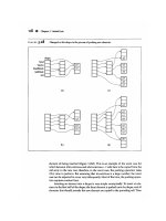
Figure 9.11: Insertion of an entry with key 42 into the
skip list of Figure 9.9
. We assume that the random
"coin flips" for the new entry came up heads three
times in a row, followed by tails. The positions visited
are highlighted in blue. The positions inserted to hold

562
the new entry are drawn with thick lines, and the
positions preceding them are flagged.

Removal in a Skip List
Like the search and insertion algorithms, the removal algorithm for a skip list is
quite simple. In fact, it is even easier than the insertion algorithm. That is, to
perform a remove(k) operation, we begin by executing method
SkipSearch(k). If the position p stores an entry with key different from k, we
return null. Otherwise, we remove p and all the positions above p, which are
easily accessed by using above operations to climb up the tower of this entry in
S starting at position p. The removal algorithm is illustrated in Figure 9.12 and a
detailed description of it is left as an exercise (R-9.16). As we show in the next
subsection, operation remove in a skip list with n entries has O(logn) expected
running time.
Before we give this analysis, however, there are some minor improvements to the
skip list data structure we would like to discuss. First, we don't actually need to
store references to entries at the levels of the skip list above the bottom level,
because all that is needed at these levels are references to keys. Second, we don't
actually need the above method. In fact, we don't need the prev method either.
We can perform entry insertion and removal in strictly a top-down, scan-forward
fashion, thus saving space for "up" and "prev" references. We explore the details

of this optimization in Exercise C-9.10
. Neither of these optimizations improve
the asymptotic performance of skip lists by more than a constant factor, but these
improvements can, nevertheless, be meaningful in practice. In fact, experimental
evidence suggests that optimized skip lists are faster in practice than AVL trees
and other balanced search trees, which are discussed in Chapter 10
.
The expected running time of the removal algorithm is O(logn), which we show
in Section 9.4.2.

Figure 9.12: Removal of the entry with key 25 from
the skip list of Figure 9.11
. The positions visited after

563
the search for the position of S
0
holding the entry are
highlighted in blue. The positions removed are drawn
with dashed lines.

Maintaining the Top-most Level
A skip-list S must maintain a reference to the start position (the top-most, left
position in S) as an instance variable, and must have a policy for any insertion that
wishes to continue inserting a new entry past the top level of S. There are two
possible courses of action we can take, both of which have their merits.
One possibility is to restrict the top level, h, to be kept at some fixed value that is
a function of n, the number of entries currently in the dictionary (from the
analysis we will see that h = max{ 10,2 log n} is a reasonable choice, and
picking h = 3 logn is even safer). Implementing this choice means that we

must modify the insertion algorithm to stop inserting a new position once we
reach the top-most level (unless logn < log(n + 1), in which case we can
now go at least one more level, since the bound on the height is increasing).
The other possibility is to let an insertion continue inserting a new position as
long as heads keeps getting returned from the random number generator. This is
the approach taken in Algorithm SkipInsert of Code Fragment 9.11
. As we
show in the analysis of skip lists, the probability that an insertion will go to a level
that is more than O(logn) is very low, so this design choice should also work.
Either choice will still result in the expected O(logn) time to perform search,
insertion, and removal, however, which we show in the next section.
9.4.2 A Probabilistic Analysis of Skip Lists 
As we have shown above, skip lists provide a simple implementation of an ordered
dictionary. In terms of worst-case performance, however, skip lists are not a
superior data structure. In fact, if we don't officially prevent an insertion from
continuing significantly past the current highest level, then the insertion algorithm

564
can go into what is almost an infinite loop (it is not actually an infinite loop,
however, since the probability of having a fair coin repeatedly come up heads
forever is 0). Moreover, we cannot infinitely add positions to a list without
eventually running out of memory. In any case, if we terminate position insertion at
the highest level h, then the worst-case running time for performing the find,
insert, and remove operations in a skip list S with n entries and height h is O(n
+ h). This worst-case performance occurs when the tower of every entry reaches
level h−1, where h is the height of S. However, this event has very low probability.
Judging from this worst case, we might conclude that the skip list structure is
strictly inferior to the other dictionary implementations discussed earlier in this
chapter. But this would not be a fair analysis, for this worst-case behavior is a gross
overestimate.

Bounding the Height of a Skip List
Because the insertion step involves randomization, a more accurate analysis of
skip lists involves a bit of probability. At first, this might seem like a major
undertaking, for a complete and thorough probabilistic analysis could require
deep mathematics (and, indeed, there are several such deep analyses that have
appeared in data structures research literature). Fortunately, such an analysis is
not necessary to understand the expected asymptotic behavior of skip lists. The
informal and intuitive probabilistic analysis we give below uses only basic
concepts of probability theory.
Let us begin by determining the expected value of the height h of a skip list S with
n entries (assuming that we do not terminate insertions early). The probability that
a given entry has a tower of height i ≥ 1 is equal to the probability of getting i
consecutive heads when flipping a coin, that is, this probability is 1/2
i
. Hence, the
probability PP
i
that level i has at least one position is at most
P
i
≤ n/2
i
,
for the probability that any one of n different events occurs is at most the sum of
the probabilities that each occurs.
The probability that the height h of S is larger than i is equal to the probability that
level i has at least one position, that is, it is no more than P
i
This means that h is
larger than, say, 3 log n with probability at most

P
3 log n
≤ n/2
3 log n

= n/n
3
= 1/n
2
.
For example, if n = 1000, this probability is a one-in-a-million long shot. More
generally, given a constant c > 1, h is larger than c log n with probability at most
1/n
c−1
. That is, the probability that h is smaller than c log n is at least 1 − 1/n
c−1
.
Thus, with high probability, the height h of S is O(logn).

565
Analyzing Search Time in a Skip List
Next, consider the running time of a search in skip list S, and recall that such a
search involves two nested while loops. The inner loop performs a scan forward
on a level of S as long as the next key is no greater than the search key k, and the
outer loop drops down to the next level and repeats the scan forward iteration.
Since the height h of S is O(logn) with high probability, the number of drop-down
steps is O(logn) with high probability.
So we have yet to bound the number of scan-forward steps we make. Let n
i
be the

number of keys examined while scanning forward at level i. Observe that, after
the key at the starting position, each additional key examined in a scan-forward at
level i cannot also belong to level i+1. If any of these keys were on the previous
level, we would have encountered them in the previous scan-forward step. Thus,
the probability that any key is counted in n
i
is 1/2. Therefore, the expected value
of n
i
is exactly equal to the expected number of times we must flip a fair coin
before it comes up heads. This expected value is 2. Hence, the expected amount
of time spent scanning forward at any level i is O(1). Since S has O(logn) levels
with high probability, a search in S takes expected time O(logn). By a similar
analysis, we can show that the expected running time of an insertion or a removal
is O(logn).
Space Usage in a Skip List
Finally, let us turn to the space requirement of a skip list S with n entries. As we
observed above, the expected number of positions at level i is n/2
i
, which means
that the expected total number of positions in S is
.
Using Proposition 4.5 on geometric summations, we have
for all h ≥ 0.
Hence, the expected space requirement of S is O(n).
Table 9.4 summarizes the performance of a dictionary realized by a skip list.
Table 9.4: Performance of a dictionary
implemented with a skip list. We denote the number

566

of entries in the dictionary at the time the operation is
performed with n, and the size of the collection
returned by operation findAll with s. The expected
space requirement is O(n).
Operation
Time
size, isEmpty
O(1)
entries
O(n)
find, insert, remove
O(logn) (expected)
findAll
O(logn + s) (expected)
9.5 Extensions and Applications of Dictionaries
In this section, we explore several extensions and applications of dictionaries.
9.5.1 Supporting Location-Aware Dictionary Entries
As we did for priority queues (Section 8.4.2), we can also use location-aware
entries to speed up the running time for some operations in a dictionary. In
particular, a location-aware entry can greatly speed up entry removal in a
dictionary. For in removing a location-aware entry e, we can simply go directly to
the place in our data structure where we are storing e and remove it. We could
implement a location-aware entry, for example, by augmenting our entry class with
a private location variable and protected methods, location() and
setLocation(p), which return and set this variable respectively. We then require
that the location variable for an entry e, always refer to e's position or index in
the data structure implementing our dictionary. We would, of course, have to update
this variable any time we moved an entry, so it would probably make the most
sense for this entry class to be closely related to the class implementing the
dictionary (the location-aware entry class could even be nested inside the dictionary

567
class). Below, we show how to set up location-aware entries for several data
structures presented in this chapter.
• Unordered list : In an unordered list, L, implementing a dictionary, we can
maintain the location variable of each entry e to point to e's position in the
underlying linked list for L. This choice allows us to perform remove(e) as
L.remove(e.location()), which would run in O(1) time.
• Hash table with separate chaining : Consider a hash table,
with bucket array A and hash function h, that uses separate chaining for handling
collisions. We use the location variable of each entry e to point to e's position
in the list L implementing the mini-map A[h(k)]. This choice allows us to perform
the main work of a remove(e) as L.remove(e.location()), which would
run in constant expected time.
• Ordered search table : In an ordered table, T, implementing a dictionary,
we should maintain the location variable of each entry e to be e's index in T.
This choice would allow us to perform remove(e) as
T.remove(e.location()). (Recall that location() now returns an
integer.) This approach would run fast if entry e was stored near the end of T.
• Skip list : In a skip list, S, implementing a dictionary, we should maintain
the location variable of each entry e to point to e's position in the bottom level
of S. This choice would allow us to skip the search step in our algorithm for
performing remove(e) in a skip list.
We summarize the performance of entry removal in a dictionary with location-
aware entries in Table 9.5.
Table 9.5: Performance of the remove method in
dictionaries implemented with location-aware entries.
We use n to denote the number of entries in the
dictionary.
List

Hash Table
Search Table
Skip List
O(1)
O(1) (expected)

568
O(n)
O(logn) (expected)
9.5.2 The Ordered Dictionary ADT
In an ordered dictionary, we want to perform the usual dictionary operations, but
also maintain an order relation for the keys in our dictionary. We can use a
comparator to provide the order relation among keys, as we did for the ordered
search table and skip list dictionary implementations described above. Indeed, all of
the dictionary implementations discussed in Chapter 10 use a comparator to store
the dictionary in nondecreasing key order.
When the entries of a dictionary are stored in order, we can provide efficient
implementations for additional methods in the dictionary ADT. For example, we
could consider adding the following methods to the dictionary ADT so as to define
the ordered dictionary ADT.
first(): Return an entry with smallest key.
last(): Return an entry with largest key.
successors(k): Return an iterator of the entries with keys greater than or
equal to k, in nondecreasing order.
predecessors(k): Return an iterator of the entries with keys less than or equal to
k, in nonincreasing order.
Implementing an Ordered Dictionary
The ordered nature of the operations above makes the use of an unordered list or a
hash table inappropriate for implementing the dictionary, because neither of these
data structures maintains any ordering information for the keys in the dictionary.

Indeed, hash tables achieve their best search speeds when their keys are
distributed almost at random. Thus, we should consider an ordered search table or
skip list (or a data structure from Chapter 10) when dealing with ordered
dictionaries.
for example, using a skip list to implement an ordered dictionary, we can
implement methods first() and last() in O(1) time by accessing the second
and second to last positions of the bottom list. Also methods successors(k)
and predecessors(k) can be implemented to run in O(logn) expected time.
Moreover, the iterators returned by the successors(k) and
predecessors(k) methods could be implemented using a reference to a current

569
position in the bottom level of the skip list. Thus, the hasNext and next
methods of these iterators would each run in constant time using this approach.
The java.util.Sorted Map Interface
Java provides an ordered version of the java.util.Map interface in its
interface called java.util.SortedMap. This interface extends the
java.util.Map interface with methods that take order into account. Like the
parent interface, a SortedMap does not allow for duplicate keys.
Ignoring the fact that dictionaries allow for multiple entries with the same key,
possible correspondences between methods of our ordered dictionary ADT and
methods of interface java.util.SortedMap are shown in Table 9.6.
Table 9.6: Loose correspondences between
methods of the ordered dictionary ADT and methods
of the java.util.SortedMap interface, which
supports other methods as well. The
java.util.SortedMap expression for
predecessors(k) is not an exact correspondence,
however, as the iterator returned would be by
increasing keys and would not include the entry with

key equal to k. There appears to be no efficient way of
getting a true correspondence to predecessors(k)
using java.util.SortedMap methods.
Ordered Dictionary Methods
java.util.SortedMap Methods
first().getKey()
firstKey()
first().getValue()
get(firstKey())
last().getKey()

570
lastKey()
last().getValue()
get(lastKey())
successors(k)
tailMap(k).entrySet().iterator()
predecessors(k)
headMap(k).entrySet().iterator()
9.5.3 Flight Databases and Maxima Sets
As we have mentioned in the preceding sections, unordered and ordered
dictionaries have many applications.
In this section, we explore some specific applications of ordered dictionaries.
Flight Databases
There are several web sites on the Internet that allow users to perform queries on
flight databases to find flights between various cities, typically with the intent to
buy a ticket. To make a query, a user specifies origin and destination cities, a
departure date, and a departure time. To support such queries, we can model the
flight database as a dictionary, where keys are Flight objects that contain fields
corresponding to these four parameters. That is, a key is a tuple

k = (origin, destination, date, time).
Additional information about a flight, such as the flight number, the number of
seats still available in first (F) and coach (Y) class, the flight duration, and the
fare, can be stored in the value object.
Finding a requested flight is not simply a matter of finding a key in the dictionary
matching the requested query, however. The main difficulty is that, although a
user typically wants to exactly match the origin and destination cities, as well as
the departure date, he or she will probably be content with any departure time that
is close to his or her requested departure time. We can handle such a query, of
course, by ordering our keys lexicographically. Thus, given a user query key k,
we can call successors(k) to return an iteration of all the flights between the
desired cities on the desired date, with departure times in strictly increasing order
from the requested departure time. A similar use of predecessors(k) would
give us flights with times before the requested time. Therefore, an efficient

571
implementation for an ordered dictionary, say, one that uses a skip list, would be a
good way to satisfy such queries. For example, calling successors(k) on a
query key k = (ORD, PVD, 05May, 09:30), could result in an iterator with the
following entries:
((ORD, PVD, 05May, 09:53), (AA 1840, F5, Y15, 02:05,
$251))
((ORD, PVD, 05May, 13:29), (AA 600, F2, Y0, 02:16,
$713))
((ORD, PVD, 05May, 17:39), (AA 416, F3, Y9, 02:09,
$365))
((ORD, PVD, 05May, 19:50), (AA 1828, F9, Y25, 02:13,
$186))
Maxima Sets
Life is full of trade-offs. We often have to trade off a desired performance

measure against a corresponding cost. Suppose, for the sake of an example, we
are interested in maintaining a database rating automobiles by their maximum
speeds and their cost. We would like to allow someone with a certain amount to
spend to query our database to find the fastest car they can possibly afford.
We can model such a trade-off problem as this by using a key-value pair to model
the two parameters that we are trading off, which in this case would be the pair
(cost, speed) for each car. Notice that some cars are strictly better than other
cars using this measure. For example, a car with cost-speed pair (20,000,100) is
strictly better than a car with cost-speed pair (30,000,90). At the same time, there
are some cars that are not strictly dominated by another car. For example, a car
with cost-speed pair (20000,100) may be better or worse than a car with cost-
speed pair (30000,120), depending on how much money we have to spend. (See
Figure 9.13
.)
Figure 9.13: Illustrating the cost-performance trade-
off with key-value pairs represented by points in the
plane. Notice that point p is strictly better than points
c, d, and e, but may be better or worse than points a,
b, f, g, and h, depending on the price we are willing to
pay. Thus, if we were to add p to our set, we could
remove the points c, d, and e, but not the others.

572

Formally, we say a price-performance pair (a, b) dominates a pair (c, d) if a < c
and b > d. A pair (a, b) is called a maximum pair if it is not dominated by any
other pairs. We are interested in maintaining the set of maxima of a collection C
of price-performance pairs. That is, we would like to add new pairs to this
collection (for example, when a new car is introduced), and we would like to
query this collection for a given dollar amount d to find the fastest car that costs

no more than d dollars.
We can store the set of maxima pairs in an ordered dictionary, D, ordered by cost,
so that the cost is the key field and performance (speed) is the value field. We can
then implement operations add(c,p), which adds a new cost-performance pair
(c,p), and best(c), which returns the best pair with cost at most c, as shown in
Code Fragment 9.12.
Code Fragment 9.12: The methods for maintaining
a set of maxima, as implemented with an ordered
dictionary D.

573

if we implement D using a skip list, then we can perform best(c) queries in
O(logn) expected time and add(c,p) updates in O((1 + r)log n) expected time,
where r is the number of points removed. Thus, we are able to achieve good
running times for the methods that maintain our set of maxima.
9.6 Exercises
for source code and help with exercises, please visit
java.datastructures.net.
Reinforcement
R-9.1

574
What is the worst-case running time for inserting n key-value entries into an
initially empty map M that is implemented with a list?
R-9.2
Describe how to use a map to implement the dictionary ADT, assuming that the
user does not attempt to insert entries with the same key.
R-9.3
Describe how an ordered list implemented as a doubly linked list could be used

to implement the map ADT.
R-9.4
What would be a good hash code for a vehicle identification number, that is a
string of numbers and letters of the form "9X9XX99X9XX999999," where a
"9" represents a digit and an "X" represents a letter?
R-9.5
Draw the 11-entry hash table that results from using the hash function, h(i) + (2i
+ 5) mod 11, to hash the keys 12,44, 13, 88, 23, 94, 11, 39, 20, 16, and 5,
assuming collisions are handled by chaining.
R-9.6
What is the result of the previous exercise, assuming collisions are handled by
linear probing?
R-9.7
Show the result of Exercise R-9.5
, assuming collisions are handled by quadratic
probing, up to the point where the method fails.
R-9.8
What is the result of Exercise R-9.5 when collisions are handled by double
hashing using the secondary hash function h ′(k) = 7 − (k mod 7)?
R-9.9
Give a pseudo-code description of an insertion into a hash table that uses
quadratic probing to resolve collisions, assuming we also use the trick of
replacing deleted entries with a special "deactivated entry" object.
R-9.10

575
Give a Java description of the values() and entries() methods that could
be included in the hash table implementation of Code Fragments 9.3–9.5.
R-9.11
Explain how to modify class HashTableMap given in Code Fragments 9.3

–
9.5
, so that it implements the dictionary ADT instead of the map ADT.
R-9.12
Show the result of rehashing the hash table shown in Figure 9.4
into a table of
size 19 using the new hash function h(k) = 2k mod 19.
R-9.13
Argue why a hash table is not suited to implement an ordered dictionary.
R-9.14
What is the worst-case time for putting n entries in an initially empty hash table,
with collisions resolved by chaining? What is the best case?
R-9.15
Draw an example skip list that results from performing the following series of
operations on the skip list shown in Figure 9.12
: remove(38), insert(48,x),
insert(24,y), remove(55). Record your coin flips, as well.
R-9.16
Give a pseudo-code description of the remove operation in a skip list.
R-9.17
What is the expected running time of the methods for maintaining a maxima set
if we insert n pairs such that each pair has lower cost and performance than one
before it? What is contained in the ordered dictionary at the end of this series of
operations? What if each pair had a lower cost and higher performance than the
one before it?
R-9.18
Argue why location-aware entries are not really needed for a dictionary
implemented with a good hash table.
Creativity
C-9.1

576
Describe how to use a map to implement the dictionary ADT, assuming that the
user may attempt to insert entries with the same key.
C-9.2
Suppose we are given two ordered search tables S and T, each with n entries
(with S and T being implemented with arrays). Describe an O(log
2
n)-time
algorithm for finding the kth smallest key in the union of the keys from S and T
(assuming no duplicates).
C-9.3
Give an O(logn)-time solution for the previous problem.
C-9.4
Design a variation of binary search for performing operation findAll(k) in a
dictionary implemented with an ordered search table, and show that it runs in
time O(logn + s), where n is the number of elements in the dictionary and s is
the size of the iterator returned.
C-9.5
Describe the changes that must be made in the pseudo-code descriptions of the
fundamental dictionary methods when we implement a dictionary with a hash
table such that collisions are handled via separate chaining, but we add the
space optimization that if a bucket stores just a single entry, then we simply
have the bucket reference that entry directly.
C-9.6
The hash table dictionary implementation requires that we find a prime number
between a number M and a number 2M. Implement a method for finding such a
prime by using the sieve algorithm. In this algorithm, we allocate a 2M cell
Boolean array A, such that cell i is associated with the integer i. We then
initialize the array cells to all be "true" and we "mark off all the cells that are

multiples of 2, 3, 5, 7, and so on. This process can stop after it reaches a number
larger than
. (Hint: Consider a bootstrapping method for finding the
primes up to
.)
C-9.7
Describe how to perform a removal from a hash table that uses linear probing to
resolve collisions where we do not use a special marker to represent deleted
elements. That is, we must rearrange the contents so that it appears that the
removed entry was never inserted in the first place.

577
C-9.8
Given a collection C of n cost-performance pairs (c,p), describe an algorithm for
finding the maxima pairs of C in O(n logn) time.
C-9.9
The quadratic probing strategy has a clustering problem related to the way it
looks for open slots. Namely, when a collision occurs at bucket h(k), it checks
buckets A[(h(k) + j
2
) mod N], for j = 1,2,…, N − 1.
a.
Show that j
2
mod N will assume at most (N + 1)/2 distinct values, for N
prime, as j ranges from 1 to N − 1. As a part of this justification, note that j
2

mod N = (N − j)
2

mod N for all j.
b.
A better strategy is to choose a prime N such that N mod 4 = 3 and then to
check the bucketsA[(h(k) ± j
2
) mod N] as j ranges from 1 to (N − 1)/2,
alternating between plus and minus. Show that this alternate version is
guaranteed to check every bucket in A.
C-9.10
Show that the methods above(p) and prev(p) are not actually needed to
efficiently implement a dictionary using a skip list. That is, we can implement
entry insertion and removal in a skip list using a strictly top-down, scan-forward
approach, without ever using the above or prev methods. (Hint: In the
insertion algorithm, first repeatedly flip the coin to determine the level where
you should start inserting the new entry.)
C-9.11
Describe how to implement successors(k) in an ordered dictionary realized
using an ordered search table. What is its running time?
C-9.12
Repeat the previous exercise using a skip list. What is the expected running time
in this case?
C-9.13
Suppose that each row of an n × n array A consists of 1's and 0's such that, in
any row of A, all the 1's come before any 0's in that row. Assuming A is already

578