Data Structures and Algorithms in Java 4th phần 9 doc

Partition the set S into …n/5… groups of size 5 each (except possibly for one
group). Sort each little set and identify the median element in this set. From this
set of …n/5… "baby" medians, apply the selection algorithm recursively to find
the median of the baby medians. Use this element as the pivot and proceed as in
the quick-select algorithm.
Show that this deterministic method runs in O(n) time by answering the
following questions (please ignore floor and ceiling functions if that simplifies
the mathematics, for the asymptotics are the same either way):
a.
How many baby medians are less than or equal to the chosen pivot? How
many are greater than or equal to the pivot?
b.
For each baby median less than or equal to the pivot, how many other
elements are less than or equal to the pivot? Is the same true for those
greater than or equal to the pivot?
c.
Argue why the method for finding the deterministic pivot and using it to
partition S takes O(n) time.
d.
Based on these estimates, write a recurrence equation to bound the worst-
case running time t(n) for this selection algorithm (note that in the worst
case there are two recursive calls—one to find the median of the baby
medians and one to recur on the larger of L and G).
e.
Using this recurrence equation, show by induction that t(n) is O(n).
Projects
P-11.1
Experimentally compare the performance of in-place quick-sort and a version of
quick-sort that is not in-place.
P-11.2

738
Design and implement a stable version of the bucket-sort algorithm for sorting a
sequence of n elements with integer keys taken from the range [0,N − 1], for N
≥ 2. The algorithm should run in O(n + N) time.
P-11.3
Implement merge-sort and deterministic quick-sort and perform a series of
benchmarking tests to see which one is faster. Your tests should include
sequences that are "random" as well as "almost" sorted.
P-11.4
Implement deterministic and randomized versions of the quick-sort algorithm
and perform a series of benchmarking tests to see which one is faster. Your tests
should include sequences that are very "random" looking as well as ones that
are "almost" sorted.
P-11.5
Implement an in-place version of insertion-sort and an in-place version of
quick-sort. Perform benchmarking tests to determine the range of values of n
where quick-sort is on average better than insertion-sort.
P-11.6
Design and implement an animation for one of the sorting algorithms described
in this chapter. Your animation should illustrate the key properties of this
algorithm in an intuitive manner.
P-11.7
Implement the randomized quick-sort and quick-select algorithms, and design a
series of experiments to test their relative speeds.
P-11.8
Implement an extended set ADT that includes the methods union(B),
intersect(B), subtract(B), size(), isEmpty(), plus the methods equals(B),
contains(e), insert(e), and remove(e) with obvious meaning.
P-11.9
Implement the tree-based union/find partition data structure with both the

union-by-size and path-compression heuristics.
Chapter Notes

739
Knuth's classic text on Sorting and Searching [63] contains an extensive history of
the sorting problem and algorithms for solving it. Huang and Langston [52] describe
how to merge two sorted lists in-place in linear time. Our set ADT is derived from the
set ADT of Aho, Hopcroft, and Ullman [5]
. The standard quick-sort algorithm is due
to Hoare [49]
. More information about randomization, including Chernoff bounds,
can be found in the appendix and the book by Motwani and Raghavan [79]. The
quick-sort analysis given in this chapter is a combination of an analysis given in a
previous edition of this book and the analysis of Kleinberg and Tardos [59]. The
quick-sort analysis of Exercise C-11.7
is due to Littman. Gonnet and Baeza-Yates
[41]
provide experimental comparisons and theoretical analyses of a number of
different sorting algorithms. The term "prune-and-search" comes originally from the
computational geometry literature (such as in the work of Clarkson [22] and Megiddo
[72, 73]). The term "decrease-and-conquer" is from Levitin [68].

Chapter 12 Text Processing

740

Contents
12.1
String Operations
540
12.1.1
The Java String Class
541
12.1.2
The Java StringBuffer Class
542
12.2
PatternMatching Algorithms
543
12.2.1
Brute Force
543
12.2.2
The Boyer-Moore Algorithm
545

12.2.3

741
The Knuth-Morris-Pratt Algorithm
549
12.3
Tries
554
12.3.1
Standard Tries
554
12.3.2
Compressed Tries
558
12.3.3
Suffix Tries
560
12.3.4
Search Engines
564
12.4
Text Compression
565
12.4.1
The Huffman Coding Algorithm
566
12.4.2
The Greedy Method

742

567
12.5
Text Similarity Testing
568
12.5.1
The Longest Common Subsequence Problem
568
12.5.2
Dynamic Programming
569
12.5.3
Applying Dynamic Programming to the LCS Problem
569
12.6
12.6 Exercises
573
java.datastructures.net

12.1 String Operations
Document processing is rapidly becoming one of the dominant functions of
computers. Computers are used to edit documents, to search documents, to transport
documents over the Internet, and to display documents on printers and computer
screens. For example, the Internet document formats HTML and XML are primarily
text formats, with added tags for multimedia content. Making sense of the many
terabytes of information on the Internet requires a considerable amount of text
processing.
In addition to having interesting applications, text processing algorithms also
highlight some important algorithmic design patterns. In particular, the pattern
matching problem gives rise to the brute-force method, which is often inefficient but
has wide applicability. For text compression, we can apply the greedy method, which

743
often allows us to approximate solutions to hard problems, and for some problems
(such as in text compression) actually gives rise to optimal algorithms. Finally, in
discussing text similarity, we introduce the dynamic programming design pattern,
which can be applied in some special instances to solve a problem in polynomial time
that appears at first to require exponential time to solve.
Text Processing
At the heart of algorithms for processing text are methods for dealing with character
strings. Character strings can come from a wide variety of sources, including
scientific, linguistic, and Internet applications. Indeed, the following are examples
of such strings:
P = "CGTAAACTGCTTTAATCAAACGC"
S = "".
The first string, P, comes from DNA applications, and the second string, S, is the
Internet address (URL) for the Web site that accompanies this book.
Several of the typical string processing operations involve breaking large strings
into smaller strings. In order to be able to speak about the pieces that result from
such operations, we use the term substring of an m-character string P to refer to a
string of the form P[i]P[i + 1]P[i + 2] … P[j], for some 0 ≤ i ≤ j ≤ m− 1, that is, the
string formed by the characters in P from index i to index j, inclusive. Technically,
this means that a string is actually a substring of itself (taking i = 0 and j = m − 1),
so if we want to rule this out as a possibility, we must restrict the definition to
proper substrings, which require that either i > 0 or j − 1.
To simplify the notation for referring to substrings, let us use P[i j] to denote the
substring of P from index i to index j, inclusive. That is,
P[i j]=P[i]P[i+1]…P[j].
We use the convention that if i > j, then P[i j] is equal to the null string, which has
length 0. In addition, in order to distinguish some special kinds of substrings, let us
refer to any substring of the form P [0 i], for 0 ≤ i ≤ m −1, as a prefix of P, and any

substring of the form P[i m − 1], for 0 ≤ i ≤ m − 1, as a suffix of P. For example, if
we again take P to be the string of DNA given above, then "CGTAA" is a prefix of
P, "CGC" is a suffix of P, and "TTAATC" is a (proper) substring of P. Note that the
null string is a prefix and a suffix of any other string.
To allow for fairly general notions of a character string, we typically do not restrict
the characters in T and P to explicitly come from a well-known character set, like
the Unicode character set. Instead, we typically use the symbol σ to denote the
character set, or alphabet, from which characters can come. Since most document
processing algorithms are used in applications where the underlying character set is

744
finite, we usually assume that the size of the alphabet σ, denoted with |σ|, is a fixed
constant.
String operations come in two flavors: those that modify the string they act on and
those that simply return information about the string without actually modifying it.
Java makes this distinction precise by defining the String class to represent
immutable strings, which cannot be modified, and the StringBuffer class to
represent mutable strings, which can be modified.
12.1.1 The Java String Class
The main operations of the Java String class are listed below:
length():
Return the length, n, of S.
charAt(i):
Return the character at index i in S.
startsWith(Q):
Determine if Q is a prefix of S.
endsWith(Q):
Determine if Q is a suffix of S.
substring(i,j):
Return the substring S[i,j].

concat(Q):
Return the concatenation of S and Q, that is, S+Q.
equals(Q):
Determine if Q is equal to S.
indexOf(Q):
If Q is a substring of S, return the index of the beginning of the first
occurrence of Q in S, else return −1.
This collection forms the typical operations for immutable strings.

745
Example 12.1: Consider the following set of operations, which are performed
on the string S = "abcdefghijklmnop":
Operation
Output
length()
16
charAt(5)
'f'
concat("qrs")
"abcdefghijklmnopqrs"
endsWith("javapop")
false
indexOf("ghi")
6
startsWith("abcd")
true
substring(4,9)
"efghij"
With the exception of the indexOf(Q) method, which we discuss in Section 12.2
,

all the methods above are easily implemented simply by representing the string as
an array of characters, which is the standard String implementation in Java.
12.1.2 The Java StringBuffer Class
The main methods of the Java StringBuffer class are listed below:
append(Q):
Return S+Q, replacing S with S + Q.
insert(i, Q):

746
Return and update S to be the string obtained by inserting Q inside S
starting at index i.
reverse():
Reverse and return the string S.
setCharAt(i,ch):
Set the character at index i in S to be ch.
charAt(i):
Return the character at index i in S.
Error conditions occur when the index i is out of the bounds of the indices of the
string. With the exception of the charAt method, most of the methods of the
String class are not immediately available to a StringBuffer object S in
Java. Fortunately, the Java StringBuffer class provides a toString()
method that returns a String version of S, which can be used to access String
methods.
Example 12.2: Consider the following sequence of operations, which are
performed on the mutable string that is initially S = abcdefghijklmnop":
Operation
S
append("qrs")
"abcdefghijklmnopqrs"
insert(3,"xyz")

"abcxyzdefghijklmnopqrs"
reverse()
"srqponmlkjihgfedzyxcba"
setCharAt(7,'W')
"srqponmWkjihgfedzyxcba"
12.2 Pattern Matching Algorithms

747
In the classic pattern matching problem on strings, we are given a text string T of
length n and apattern string P of length m, and want to find whether P is a substring
of T. The notion of a "match" is that there is a substring of T starting at some index i
that matches P, character by character, so that T[i] = P[0], T[i + 1] = P[1], …, T[i +
m− 1] = P[m − 1]. That is, P = T[i i + m − 1]. Thus, the output from a pattern
matching algorithm could either be some indication that the pattern P does not exist
in T or an integer indicating the starting index in T of a substring matching P. This is
exactly the computation performed by the indexOf method of the Java String
interface. Alternatively, one may want to find all the indices where a substring of T
matching P begins.
In this section, we present three pattern matching algorithms (with increasing levels
of difficulty).
12.2.1 Brute Force.
The brute force algorithmic design pattern is a powerful technique for algorithm
design when we have something we wish to search for or when we wish to optimize
some function. In applying this technique in a general situation we typically
enumerate all possible configurations of the inputs involved and pick the best of all
these enumerated configurations.
In applying this technique to design the brute-force pattern matching algorithm,
we derive what is probably the first algorithm that we might think of for solving the
pattern matching problem—we simply test all the possible placements of P relative
to T. This algorithm, shown in Code Fragment 12.1, is quite simple.

Algorithm BruteForceMatch(T,P): Input: Strings T (text) with n characters and P
(pattern) with m characters Output: Starting index of the first substring of T
matching P, or an indication that P is not a substring of T for i ← 0 to n − m {for
each candidate index in T} do j ← 0 while (j and T[i + j] = P[j]) do j ← j + 1 if j =
m then return i return "There is no substring of T matching P."
Code Fragment 12.1: Brute-force pattern matching.

748

Performance
The brute-force pattern matching algorithm could not be simpler. It consists of
two nested loops, with the outer loop indexing through all possible starting
indices of the pattern in the text, and the inner loop indexing through each
character of the pattern, comparing it to its potentially corresponding character in
the text. Thus, the correctness of the brute-force pattern matching algorithm
follows immediately from this exhaustive search approach.
The running time of brute-force pattern matching in the worst case is not good,
however, because, for each candidate index in T, we can perform up to m
character comparisons to discover that P does not match T at the current index.
Referring to Code Fragment 12.1, we see that the outer for loop is executed at
most n − m+ 1 times, and the inner loop is executed at most m times. Thus, the
running time of the brute-force method is O((n − m+ 1)m), which is simplified as
O(nm). Note that when m = n/2, this algorithm has quadratic running time O(n
2
).
Example 12.3: Suppose we are given the text string
T = "abacaabaccabacabaabb"
and the pattern string
P= "abacab".
In Figure 12.1

we illustrate the execution of the brute-force pattern matching
algorithm on T and P.
Figure 12.1: Example run of the brute-force pattern
matching algorithm. The algorithm performs 27
character comparisons, indicated above with numerical
labels.

749

12.2.2 The Boyer-Moore Algorithm
At first, we might feel that it is always necessary to examine every character in T in
order to locate a pattern P as a substring. But this is not always the case, for the
Boyer-Moore (BM) pattern matching algorithm, which we study in this section, can
sometimes avoid comparisons between P and a sizable fraction of the characters in
T. The only caveat is that, whereas the brute-force algorithm can work even with a
potentially unbounded alphabet, the BM algorithm assumes the alphabet is of fixed,
finite size. It works the fastest when the alphabet is moderately sized and the pattern
is relatively long. Thus, the BM algorithm is ideal for searching words in
documents. In this section, we describe a simplified version of the original
algorithm by Boyer and Moore.
The main idea of the BM algorithm is to improve the running time of the brute-
force algorithm by adding two potentially time-saving heuristics. Roughly stated,
these heuristics are as follows:
Looking-Glass Heuristic: When testing a possible placement of P against T, begin
the comparisons from the end of P and move backward to the front of P.
Character-Jump Heuristic: During the testing of a possible placement of P against
T, a mismatch of text character T[i] = c with the corresponding pattern character
P[j] is handled as follows. If c is not contained anywhere in P, then shift P
completely past T[i] (for it cannot match any character in P). Otherwise, shift P
until an occurrence of character c in P gets aligned with T[i].

750
We will formalize these heuristics shortly, but at an intuitive level, they work as an
integrated team. The looking-glass heuristic sets up the other heuristic to allow us to
avoid comparisons between P and whole groups of characters in T. In this case at
least, we can get to the destination faster by going backwards, for if we encounter a
mismatch during the consideration of P at a certain location in T, then we are likely
to avoid lots of needless comparisons by significantly shifting P relative to T using
the character-jump heuristic. The character-jump heuristic pays off big if it can be
applied early in the testing of a potential placement of P against T.
Let us therefore get down to the business of defining how the character-jump
heuristics can be integrated into a string pattern matching algorithm. To implement
this heuristic, we define a function last(c) that takes a character c from the
alphabet and characterizes how far we may shift the pattern P if a character equal to
c is found in the text that does not match the pattern. In particular, we define
last(c) as
• If c is in P, last(c) is the index of the last (right-most) occurrence of c in P.
Otherwise, we conventionally define last(c) = − 1.
If characters can be used as indices in arrays, then the last function can be easily
implemented as a look-up table. We leave the method for computing this table in
O(m+|σ|) time, given P, as a simple exercise (R-12.6). This last function will give
us all the information we need to perform the character-jump heuristic.
In Code Fragment 12.2, we show the BM pattern matching algorithm.
Code Fragment 12.2: The Boyer-Moore pattern
matching algorithm.

751

The jump step is illustrated in Figure 12.2.
Figure 12.2: Illustration of the jump step in the

algorithm of Code Fragment 12.2
, where we let l =
last(T[i]). We distinguish two cases: (a) 1 +l ≤ j,
where we shift the pattern by j − l units; (b) j < 1 + l,
where we shift the pattern by one unit.

752

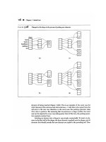
In Figure 12.3, we illustrate the execution of the Boyer-Moore pattern matching
algorithm on an input string similar to Example 12.3.
Figure 12.3: An illustration of the BM pattern
matching algorithm. The algorithm performs 13
character comparisons, which are indicated with
numerical labels.

753

The correctness of the BM pattern matching algorithm follows from the fact that
each time the method makes a shift, it is guaranteed not to "skip" over any possible
matches. For last(c) is the location of the last occurrence of c in P.
The worst-case running time of the BM algorithm is O(nm+|σ|). Namely, the
computation of the last function takes time O(m+|σ|) and the actual search for the
pattern takes O(nm) time in the worst case, the same as the brute-force algorithm.
An example of a text-pattern pair that achieves the worst case is



The worst-case performance, however, is unlikely to be achieved for English text,
for, in this case, the BM algorithm is often able to skip large portions of text. (See
Figure 12.4

.) Experimental evidence on English text shows that the average number
of comparisons done per character is 0.24 for a five-character pattern string.
Figure 12.4: An example of a Boyer-Moore execution
on English text.

754

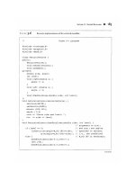
A Java implementation of the BM pattern matching algorithm is shown in Code
Fragment 12.3.
Code Fragment 12.3: Java implementation of the
BM pattern matching algorithm. The algorithm is
expressed by two static methods: Method BMmatch
performs the matching and calls the auxiliary method
build LastFunction to compute the last function,
expressed by an array indexed by the ASCII code of the
character. Method BMmatch indicates the absence of a
match by returning the conventional value − 1.

755

We have actually presented a simplified version of the Boyer-Moore (BM)
algorithm. The original BM algorithm achieves running time O(n + m + |σ|) by

756
using an alternative shift heuristic to the partially matched text string, whenever it
shifts the pattern more than the character-jump heuristic. This alternative shift
heuristic is based on applying the main idea from the Knuth-Morris-Pratt pattern
matching algorithm, which we discuss next.
12.2.3 The Knuth-Morris-Pratt Algorithm
In studying the worst-case performance of the brute-force and BM pattern matching

algorithms on specific instances of the problem, such as that given in Example 12.3,
we should notice a major inefficiency. Specifically, we may perform many
comparisons while testing a potential placement of the pattern against the text, yet if
we discover a pattern character that does not match in the text, then we throw away
all the information gained by these comparisons and start over again from scratch
with the next incremental placement of the pattern. The Knuth-Morris-Pratt (or
"KMP") algorithm, discussed in this section, avoids this waste of information and,
in so doing, it achieves a running time of O(n + m), which is optimal in the worst
case. That is, in the worst case any pattern matching algorithm will have to examine
all the characters of the text and all the characters of the pattern at least once.
The Failure Function
The main idea of the KMP algorithm is to preprocess the pattern string P so as to
compute failure function f that indicates the proper shift of P so that, to the
largest extent possible, we can reuse previously performed comparisons.
Specifically, the failure function f(j) is defined as the length of the longest prefix
of P that is a suffix of P[1 j] (note that we did not put P[0 j] here). We also use
the convention that f(0) = 0. Later, we will discuss how to compute the failure
function efficiently. The importance of this failure function is that it "encodes"
repeated substrings inside the pattern itself.
Example 12.4: Consider the pattern string P = "abacab" from Example 12.3.
The Knuth-Morris-Pratt (KMP) failure function f(j) for the string P is as shown in
the following table:

The KMP pattern matching algorithm, shown in Code Fragment 12.4
,
incrementally processes the text string T comparing it to the pattern string P. Each
time there is a match, we increment the current indices. On the other hand, if there
is a mismatch and we have previously made progress in P, then we consult the
failure function to determine the new index in P where we need to continue
checking P against T. Otherwise (there was a mismatch and we are at the

757
beginning of P), we simply increment the index for T (and keep the index variable
for P at its beginning). We repeat this process until we find a match of P in T or
the index for T reaches n, the length of T (indicating that we did not find the
pattern PinT).
Code Fragment 12.4: The KMP pattern matching
algorithm.

The main part of the KMP algorithm is the while loop, which performs a
comparison between a character in T and a character in P each iteration.
Depending upon the outcome of this comparison, the algorithm either moves on
to the next characters in T and P, consults the failure function for a new candidate
character in P, or starts over with the next index in T. The correctness of this
algorithm follows from the definition of the failure function. Any comparisons
that are skipped are actually unnecessary, for the failure function guarantees that
all the ignored comparisons are redundant—they would involve comparing the
same matching characters over again.
Figure 12.5: An illustration of the KMP pattern
matching algorithm. The failure function f for this
pattern is given in Example 12.4.
The algorithm
performs 19 character comparisons, which are
indicated with numerical labels.

758

In Figure 12.5, we illustrate the execution of the KMP pattern matching algorithm
on the same input strings as in Example 12.3. Note the use of the failure function
to avoid redoing one of the comparisons between a character of the pattern and a

character of the text. Also note that the algorithm performs fewer overall
comparisons than the brute-force algorithm run on the same strings (Figure 12.1).
Performance
Excluding the computation of the failure function, the running time of the KMP
algorithm is clearly proportional to the number of iterations of the while loop. For
the sake of the analysis, let us define k = i − j. Intuitively, k is the total amount by
which the pattern P has been shifted with respect to the text T. Note that
throughout the execution of the algorithm, we have k ≤ n. One of the following
three cases occurs at each iteration of the loop.
• If T[i] = P[j], then i increases by 1, and k does not change, since j also
increases by 1.
• If T[i] ≠ P[j] and j > 0, then i does not change and k increases by at least 1,
since in this case k changes from i − j to i − f(j − 1), which is an addition of j −
f(j − 1), which is positive because f(j − 1) < j.
• If T[i] ≠ P[j] and j = 0, then i increases by 1 and k increases by 1, since j
does not change.
Thus, at each iteration of the loop, either i or k increases by at least 1 (possibly
both); hence, the total number of iterations of the while loop in the KMP pattern
matching algorithm is at most 2n. Achieving this bound, of course, assumes that
we have already computed the failure function for P.

759
Constructing the KMP Failure Function
To construct the failure function, we use the method shown in Code Fragment
12.5, which is a "bootstrapping" process quite similar to the KMPMatch
algorithm. We compare the pattern to itself as in the KMP algorithm. Each time
we have two characters that match, we set f(i) = j + 1. Note that since we have i >
j throughout the execution of the algorithm, f(j − 1) is always defined when we
need to use it.
Code Fragment 12.5: Computation of the failure

function used in the KMP pattern matching algorithm.
Note how the algorithm uses the previous values of
the failure function to efficiently compute new values.

Algorithm KMPFailureFunction runs in O(m) time. Its analysis is analogous
to that of algorithm KMPMatch. Thus, we have:
Proposition 12.5: The Knuth-Morris-Pratt algorithm performs pattern
matching on a text string of length n and a pattern string of length m in O(n + m)
time.

760
A Java implementation of the KMP pattern matching algorithm is shown in Code
Fragment 12.6.
Code Fragment 12.6: Java implementation of the
KMP pattern matching algorithm. The algorithm is
expressed by two static methods: method KMPmatch
performs the matching and calls the auxiliary method
computeFailFunction to compute the failure function,
expressed by an array. Method KMPmatch indicates
the absence of a match by returning the conventional
value −1.

761


762