Data Structures and Algorithms in Java 4th phần 10 pdf

As with undirected graphs, we can explore a digraph in a systematic way with
methods akin to the depth-first search (DFS) and breadth-first search (BFS)
algorithms defined previously for undirected graphs (Sections 13.3.1 and 13.3.3).
Such explorations can be used, for example, to answer reachability questions. The
directed depth-first search and breadth-first search methods we develop in this
section for performing such explorations are very similar to their undirected
counterparts. In fact, the only real difference is that the directed depth-first search
and breadth-first search methods only traverse edges according to their respective
directions.
The directed version of DFS starting at a vertex v can be described by the recursive
algorithm in Code Fragment 13.11. (See Figure 13.9.)
Code Fragment 13.11: The Directed DFS
algorithm.

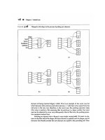
Figure 13.9: An example of a DFS in a digraph: (a)
intermediate step, where, for the first time, an already
visited vertex (DFW) is reached; (b) the completed DFS.
The tree edges are shown with solid blue lines, the back
edges are shown with dashed blue lines, and the
forward and cross edges are shown with dashed black
lines. The order in which the vertices are visited is
indicated by a label next to each vertex. The edge
(ORD,DFW) is a back edge, but (DFW,ORD) is a forward
edge. Edge (BOS,SFO) is a forward edge, and (SFO,LAX)
is a cross edge.

830

A DFS on a digraph partitions the edges of reachable from the starting
vertex into tree edges or discovery edges, which lead us to discover a new vertex,
and nontree edges, which take us to a previously visited vertex. The tree edges

form a tree rooted at the starting vertex, called the depth-first search tree, and there
are three kinds of nontree edges:
• back edges, which connect a vertex to an ancestor in the DFS tree
• forward edges, which connect a vertex to a descendent in the DFS tree
• cross edges, which connect a vertex to a vertex that is neither its ancestor
nor its descendent.
Refer back to Figure 13.9b to see an example of each type of nontree edge.
Proposition 13.16: Let be a digraph. Depth-first search on starting at
a vertex s visits all the vertices of that are reachable from s. Also, the DFS tree
contains directed paths from s to every vertex reachable from s.
Justification: Let V
s
be the subset of vertices of visited by DFS starting
at vertex s. We want to show that V
s
contains s and every vertex reachable from s
belongs to V
s
. Suppose now, for the sake of a contradiction, that there is a vertex w
reachable from s that is not in V
s
. Consider a directed path from s to w, and let (u, v)
be the first edge on such a path taking us out of V
s
, that is, u is in V
s
but v is not in
V
s
. When DFS reaches u, it explores all the outgoing edges of u, and thus must

reach also vertex v via edge (u,v). Hence, v should be in V
s
, and we have obtained a
contradiction. Therefore, V
s
must contain every vertex reachable from s

Analyzing the running time of the directed DFS method is analogous to that for its
undirected counterpart. In particular, a recursive call is made for each vertex exactly

831
once, and each edge is traversed exactly once (from its origin). Hence, if ns vertices
and ms edges are reachable from vertex s, a directed DFS starting at s runs in O(n
s

+ m
s
) time, provided the digraph is represented with a data structure that supports
constant-time vertex and edge methods. The adjacency list structure satisfies this
requirement, for example.
By Proposition 13.16, we can use DFS to find all the vertices reachable from a
given vertex, and hence to find the transitive closure of . That is, we can perform
a DFS, starting from each vertex v of , to see which vertices w are reachable
from v, adding an edge (v, w) to the transitive closure for each such w. Likewise, by
repeatedly traversing digraph with a DFS, starting in turn at each vertex, we can
easily test whether is strongly connected. Namely, is strongly connected if
each DFS visits all the vertices of
Thus, we may immediately derive the proposition that follows.
Proposition 13.17: Let be a digraph with n vertices and m edges. The
following problems can be solved by an algorithm that traverses n times using

DFS, runs in O (n(n+m)) time, and uses O(n) auxiliary space:
• Computing, for each vertex v of , the subgraph reachable from v
• Testing whether is strongly connected
• Computing the transitive closure of .
Testing for Strong Connectivity
Actually, we can determine if a directed graph is strongly connected much
faster than this, just using two depth-first searches. We begin by performing a
DFS of our directed graph starting at an arbitrary vertex s. If there is any
vertex of that is not visited by this DFS, and is not reachable from s, then the
graph is not strongly connected. So, if this first DFS visits each vertex of , then
we reverse all the edges of (using the reverse Direction method) and perform
another DFS starting at s in this "reverse" graph. If every vertex of is visited
by this second DFS, then the graph is strongly connected, for each of the vertices
visited in this DFS can reach s. Since this algorithm makes just two DFS
traversals of , it runs in O(n + m) time.

832
Directed Breadth-First Search
As with DFS, we can extend breadth-first search (BFS) to work for directed
graphs. The algorithm still visits vertices level by level and partitions the set of
edges into tree edges (or discovery edges), which together form a directed
breadth-first search tree rooted at the start vertex, and nontree edges. Unlike the
directed DFS method, however, the directed BFS method only leaves two kinds of
nontree edges: back edges, which connect a vertex to one of its ancestors, and
cross edges, which connect a vertex to another vertex that is neither its ancestor
nor its descendent. There are no forward edges, which is a fact we explore in an
Exercise (C-13.10).
13.4.2 Transitive Closure
In this section, we explore an alternative technique for computing the transitive
closure of a digraph. Let be a digraph with n vertices and m edges. We compute

the transitive closure of in a series of rounds. We initialize = . We also
arbitrarily number the vertices of as v
1
, v
2
,…, v
n
. We then begin the
computation of the rounds, beginning with round 1. In a generic round k, we
truct digraph cons starting with = and adding to the direct
edge (v
ed
v
j
) if d
i
, igraph contains both the edges (v
i
,v
K
) and (v
k
,v
j
). In thi
way, we will enforce a simple rule embodied in the proposition t
s
hat follows.
Proposition 13.18: For i=1,…,n, digraph has an edge (v
i

, v
j
) if and
only if digraph has a directed path from v
i
to v
j
, whose intermediate vertices (if
any) are in the set{v
1
,…,v
k
}. In particular, is equal to , the transitive
closure of .
Proposition 13.18
suggests a simple algorithm for computing the transitive closure
of that is based on the series of rounds we described above. This algorithm is
known as the Floyd-Warshall algorithm, and its pseudo-code is given in Code
Fragment 13.12. From this pseudo-code, we can easily analyze the running time of
the Floyd-Warshall algorithm assuming that the data structure representing G
supports methods areAdjacent and insertDirectedEdge in O(1) time. The main loop
is executed n times and the inner loop considers each of O(n
2
) pairs of vertices,
performing a constant-time computation for each one. Thus, the total running time
of the Floyd-Warshall algorithm is O(n
3
).
Code Fragment 13.12: Pseudo-code for the Floyd-
Warshall algorithm. This algorithm computes the

833
transitive closure of G by incrementally computing a
series of digraphs
, , , , where for k = 1, , n.

This description is actually an example of an algorithmic design pattern known as
dynamic programming, which is discussed in more detail in Section 12.5.2. From
the description and analysis above we may immediately derive the following
proposition.
Proposition 13.19: Let be a digraph with n vertices, and let be
represented by a data structure that supports lookup and update of adjacency
information in O(1) time. Then the Floyd-Warshall algorithm computes the
transitive closure
of in O(n
3
) time.
We illustrate an example run of the Floyd-Warshall algorithm in Figure 13.10.
Figure 13.10: Sequence of digraphs computed by the
Floyd-Warshall algorithm: (a) initial digraph
=
and numbering of the vertices; (b) digraph
; (c) ,
(d)
; (e) ; (f) . Note that = = . If
digraph
has the edges (v
i
,v
k

) and (v
k
, v
j
), but not
the edge (vi, vj), in the drawing of digraph
we show

834
edges (vi,vk) and (vk,vj) with dashed blue lines, and
edge (vi, vj) with a thick blue line.

Performance of the Floyd-Warshall Algorithm

835
The running time of the Floyd-Warshall algorithm might appear to be slower than
performing a DFS of a directed graph from each of its vertices, but this depends
upon the representation of the graph. If a graph is represented using an adjacency
matrix, then running the DFS method once on a directed graph takes O(n
2
) time
(we explore the reason for this in Exercise R-13.10
). Thus, running DFS n times
takes O(n3) time, which is no better than a single execution of the Floyd-Warshall
algorithm, but the Floyd-Warshall algorithm would be much simpler to
implement. Nevertheless, if the graph is represented using an adjacency list
structure, then running the DFS algorithm n times would take O(n(n+m)) time to
compute the transitive closure. Even so, if the graph is dense, that is, if it has
&(n
2

) edges, then this approach still runs in O(n
3
) time and is more complicated
than a single instance of the Floyd-Warshall algorithm. The only case where
repeatedly calling the DFS method is better is when the graph is not dense and is
represented using an adjacency list structure.
13.4.3 Directed Acyclic Graphs
Directed graphs without directed cycles are encountered in many applications. Such
a digraph is often referred to as a directed acyclic graph, or DAG, for short.
Applications of such graphs include the following:
• Inheritance between classes of a Java program.
• Prerequisites between courses of a degree program.
• Scheduling constraints between the tasks of a project.
Example 13.20: In order to manage a large project, it is convenient to break it
up into a collection of smaller tasks. The tasks, however, are rarely independent,
because scheduling constraints exist between them. (For example, in a house
building project, the task of ordering nails obviously precedes the task of nailing
shingles to the roof deck.) Clearly, scheduling constraints cannot have circularities,
because they would make the project impossible. (For example, in order to get a job
you need to have work experience, but in order to get work experience you need to
have a job.) The scheduling constraints impose restrictions on the order in which
the tasks can be executed. Namely, if a constraint says that task a must be
completed before task b is started, then a must precede b in the order of execution
of the tasks. Thus, if we model a feasible set of tasks as vertices of a directed graph,
and we place a directed edge from v tow whenever the task for v must be executed
before the task for w, then we define a directed acyclic graph.
The example above motivates the following definition. Let
be a digraph with n
vertices. A topological ordering of
is an ordering v

1
, ,v
n
of the vertices of
such that for every edge (vi, vj) of
, i < j. That is, a topological ordering is an

836
ordering such that any directed path in G traverses vertices in increasing order. (See
Figure 13.11.) Note that a digraph may have more than one topological ordering.
Figure 13.11: Two topological orderings of the same
acyclic digraph.

Proposition 13.21: has a topological ordering if and only if it is acyclic.
Justification: The necessity (the "only if" part of the statement) is easy to
demonstrate. Suppose
is topologically ordered. Assume, for the sake of a
contradiction, that has a cycle consisting of edges (vi
0
, vi
1
), (vi
1
, vi
2
),…, (vik−
1
, vi
0
). Because of the topological ordering, we must have i

0
< i
1
< ik−
1
< i
0
,
which is clearly impossible. Thus, must be acyclic.
We now argue the sufficiency of the condition (the "if" part). Suppose is
acyclic. We will give an algorithmic description of how to build a topological
ordering for
. Since is acyclic, must have a vertex with no incoming edges
(that is, with in-degree 0). Let v
1
be such a vertex. Indeed, if v
1
did not exist, then
in tracing a directed path from an arbitrary start vertex we would eventually
encounter a previously visited vertex, thus contradicting the acyclicity of
. If we
remove v
1
from , together with its outgoing edges, the resulting digraph is sti
acyclic. Hence, the resulting digraph also has a vertex with no incoming edges, and
we let v
ll
2
be such a vertex. By repeating this process until the digraph becomes

837
empty, we obtain an ordering v
1
, ,v
n
of the vertices of . Because of the
construction above, if ( ,vj) is an edge of vi , then vi must be deleted before vj can
be deleted, and thus i<j. Thus, v
1
, , vn is a topological ordering.

Proposition 13.21 's justification suggests an algorithm (Code Fragment 13.13),
called topological sorting, for computing a topological ordering of a digraph.
Code Fragment 13.13: Pseudo-code for the
topological sorting algorithm. (We show an example
application of this algorithm in Figure 13.12
).

Proposition 13.22: Let be a digraph with n vertices andm edges. The
topological sorting algorithm runs in O(n + m) time using O(n) auxiliary space, and
either computes a topological ordering of
or fails to number some vertices,
which indicates that
has a directed cycle.

838
Justification: The initial computation of in-degrees and setup of the
incounter variables can be done with a simple traversal of the graph, which takes
O(n + m) time. We use the decorator pattern to associate counter attributes with the
vertices. Say that a vertex u is visited by the topological sorting algorithm when u is

removed from the stack S. A vertex u can be visited only when incounter (u) = 0,
which implies that all its predecessors (vertices with outgoing edges into u) were
previously visited. As a consequence, any vertex that is on a directed cycle will
never be visited, and any other vertex will be visited exactly once. The algorithm
traverses all the outgoing edges of each visited vertex once, so its running time is
proportional to the number of outgoing edges of the visited vertices. Therefore, the
algorithm runs in O(n + m) time. Regarding the space usage, observe that the stack
S and the incounter variables attached to the vertices use O(n) space.

As a side effect, the topological sorting algorithm of Code Fragment 13.13 also tests
whether the input digraph is acyclic. Indeed, if the algorithm terminates without
ordering all the vertices, then the subgraph of the vertices that have not been
ordered must contain a directed cycle.
Figure 13.12: Example of a run of algorithm
TopologicalSort (Code Fragment 13.13
): (a) initial
configuration; (b-i) after each while-loop iteration. The
vertex labels show the vertex number and the current
incounter value. The edges traversed are shown with
dashed blue arrows. Thick lines denote the vertex and
edges examined in the current iteration.

839

13.5 Weighted Graphs
As we saw in Section 13.3.3, the breadth-first search strategy can be used to find a
shortest path from some starting vertex to every other vertex in a connected graph.
This approach makes sense in cases where each edge is as good as any other, but
there are many situations where this approach is not appropriate. For example, we
might be using a graph to represent a computer network (such as the Internet), and we

might be interested in finding the fastest way to route a data packet between two

840
computers. In this case, it is probably not appropriate for all the edges to be equal to
each other, for some connections in a computer network are typically much faster
than others (for example, some edges might represent slow phone-line connections
while others might represent high-speed, fiber-optic connections). Likewise, we
might want to use a graph to represent the roads between cities, and we might be
interested in finding the fastest way to travel cross-country. In this case, it is again
probably not appropriate for all the edges to be equal to each other, for some intercity
distances will likely be much larger than others. Thus, it is natural to consider graphs
whose edges are not weighted equally.
A weighted graph is a graph that has a numeric (for example, integer) label w(e)
associated with each edge e, called the weight of edge e. We show an example of a
weighted graph in Figure 13.13.
Figure 13.13: A weighted graph whose vertices
represent major U.S. airports and whose edge weights
represent distances in miles. This graph has a path from
JFK to LAX of total weight 2,777 (going through ORD and
DFW). This is the minimum weight path in the graph
from JFK to LAX.

In the remaining sections of this chapter, we study weighted graphs.
13.6 Shortest Paths
Let G be a weighted graph. The length (or weight) of a path is the sum of the weights
of the edges of P. That is, if P = ((v
0
,v
1
),(v

1
,v
2
), , (vk
−1
,vk)), then the length of P,
denoted w(P), is defined as


841

The distance from a vertex v to a vertex U in G, denoted d(v, U), is the length of a
minimum length path (also called shortest path) from v to u, if such a path exists.
People often use the convention that d(v, u) = +∞ if there is no path at all from v to u
in G. Even if there is a path from v to u in G, the distance from v to U may not be
defined, however, if there is a cycle in G whose total weight is negative. For example,
suppose vertices in G represent cities, and the weights of edges in G represent how
much money it costs to go from one city to another. If someone were willing to
actually pay us to go from say JFK to ORD, then the "cost" of the edge (JFK,ORD)
would be negative. If someone else were willing to pay us to go from ORD to JFK,
then there would be a negative-weight cycle in G and distances would no longer be
defined. That is, anyone could now build a path (with cycles) in G from any city A to
another city B that first goes to JFK and then cycles as many times as he or she likes
from JFK to ORD and back, before going on to B. The existence of such paths would
allow us to build arbitrarily low negative-cost paths (and, in this case, make a fortune
in the process). But distances cannot be arbitrarily low negative numbers. Thus, any
time we use edge weights to represent distances, we must be careful not to introduce
any negative-weight cycles.
Suppose we are given a weighted graph G, and we are asked to find a shortest path
from some vertex v to each other vertex in G, viewing the weights on the edges as

distances. In this section, we explore efficient ways of finding all such shortest paths,
if they exist. The first algorithm we discuss is for the simple, yet common, case when
all the edge weights in G are nonnegative (that is, w(e) ≥ 0 for each edge e of G);
hence, we know in advance that there are no negative-weight cycles in G. Recall that
the special case of computing a shortest path when all weights are equal to one was
solved with the BFS traversal algorithm presented in Section 13.3.3.

There is an interesting approach for solving this single-source problem based on the
greedy method design pattern (Section 12.4.2
). Recall that in this pattern we solve the
problem at hand by repeatedly selecting the best choice from among those available
in each iteration. This paradigm can often be used in situations where we are trying to
optimize some cost function over a collection of objects. We can add objects to our
collection, one at a time, always picking the next one that optimizes the function from
among those yet to be chosen.
13.6.1 Dijkstra's Algorithm
The main idea in applying the greedy method pattern to the single-source shortest-
path problem is to perform a "weighted" breadth-first search starting at v. In
particular, we can use the greedy method to develop an algorithm that iteratively
grows a "cloud" of vertices out of v, with the vertices entering the cloud in order of

842
their distances from v. Thus, in each iteration, the next vertex chosen is the vertex
outside the cloud that is closest to v. The algorithm terminates when no more
vertices are outside the cloud, at which point we have a shortest path from v to
every other vertex of G. This approach is a simple, but nevertheless powerful,
example of the greedy method design pattern.
A Greedy Method for Finding Shortest Paths
Applying the greedy method to the single-source, shortest-path problem, results in
an algorithm known as Dijkstra's algorithm. When applied to other graph

problems, however, the greedy method may not necessarily find the best solution
(such as in the so-called traveling salesman problem, in which we wish to find
the shortest path that visits all the vertices in a graph exactly once). Nevertheless,
there are a number of situations in which the greedy method allows us to compute
the best solution. In this chapter, we discuss two such situations: computing
shortest paths and constructing a minimum spanning tree.
In order to simplify the description of Dijkstra's algorithm, we assume, in the
following, that the input graph G is undirected (that is, all its edges are
undirected) and simple (that is, it has no self-loops and no parallel edges). Hence,
we denote the edges of G as unordered vertex pairs (u,z).
In Dijkstra's algorithm for finding shortest paths, the cost function we are trying
to optimize in our application of the greedy method is also the function that we
are trying to compute—the shortest path distance. This may at first seem like
circular reasoning until we realize that we can actually implement this approach
by using a "bootstrapping" trick, consisting of using an approximation to the
distance function we are trying to compute, which in the end will be equal to the
true distance.
Edge Relaxation
Let us define a label D[u] for each vertex u in V, which we use to approximate the
distance in G from v to u. The meaning of these labels is that D[u] will always
store the length of the best path we have found so far from v to U. Initially, D[v]
= 0 and D[u] = +∞ for each u, ≠≠ v, and we define the set C, which is our
"cloud" of vertices, to initially be the empty set t. At each iteration of the
algorithm, we select a vertex u not in C with smallest D[u] label, and we pull u
into C. In the very first iteration we will, of course, pull v into C. Once a new
vertex u is pulled into C, we then update the label D[z] of each vertex z that is
adjacent to u and is outside of C, to reflect the fact that there may be a new and
better way to get to z via u. This update operation is known as a relaxation
procedure, for it takes an old estimate and checks if it can be improved to get
closer to its true value. (A metaphor for why we call this a relaxation comes from

a spring that is stretched out and then "relaxed" back to its true resting shape.) In
the case of Dijkstra's algorithm, the relaxation is performed for an edge (u,z) such

843
that we have computed a new value of D[u] and wish to see if there is a better
value for D[z] using the edge (u,z). The specific edge relaxation operation is as
follows:
Edge Relaxation:
if D[u] +w((u,z)) D[z] then
D[z]←D[u]+w((u,z))
We give the pseudo-code for Dijkstra's algorithm in Code Fragment 13.14. Note
that we use a priority queue Q to store the vertices outside of the cloud C.
Code Fragment 13.14: Dijkstra's algorithm for the
single-source shortest path problem.

We illustrate several iterations of Dijkstra's algorithm in Figures 13.14
and 13.15.
Figure 13.14: An execution of Dijkstra's algorithm on a
weighted graph. The start vertex is BWI. A box next to
each vertex v stores the label D[v]. The symbol • is
used instead of +∞. The edges of the shortest-path
tree are drawn as thick blue arrows, and for each
vertex u outside the "cloud" we show the current best

844
edge for pulling in u with a solid blue line. (Continues
in Figure 13.15
).

Figure 13.15: An example execution of Dijkstra's

algorithm. (Continued from Figure 13.14
.)

845

Why It Works
The interesting, and possibly even a little surprising, aspect of the Dijkstra
algorithm is that, at the moment a vertex u is pulled into C, its label D[u] stores
the correct length of a shortest path from v to u. Thus, when the algorithm
terminates, it will have computed the shortest-path distance from v to every vertex
of G. That is, it will have solved the single-source shortest path problem.
It is probably not immediately clear why Dijkstra's algorithm correctly finds the
shortest path from the start vertex v to each other vertex u in the graph. Why is it
that the distance from v to u is equal to the value of the label D[u] at the time
vertex u is pulled into the cloud C (which is also the time u is removed from the
priority queue Q)? The answer to this question depends on there being no
negative-weight edges in the graph, for it allows the greedy method to work
correctly, as we show in the proposition that follows.

846
Proposition 13.23: In Dijkstra's algorithm, whenever a vertex u is pulled
into the cloud, the label D[u] is equal to d(v, u), the length of a shortest path from
v to u.
Justification: Suppose that D[t]>d(v,t) for some vertex t in V, and let u be
the first vertex the algorithm pulled into the cloud C (that is, removed from Q)
such that D[u]>d(v,u). There is a shortest path P from v to u (for otherwise d(v,
u)=+∞ = D[u]). Let us therefore consider the moment when u is pulled into C, and
let z be the first vertex of P (when going from v to u) that is not in C at this
moment. Let y be the predecessor of z in path P (note that we could have y = v).
(See Figure 13.16). We know, by our choice of z, that y is already in C at this

point. Moreover, D[y] = d(v,y), since u is the first incorrect vertex. When y was
pulled into C, we tested (and possibly updated) D[z] so that we had at that point
D[z]≤D[y]+w((y,z))=d(v,y)+w((y,z)).
But since z is the next vertex on the shortest path from v to u, this implies that
D[z] = d(v,z).
But we are now at the moment when we are picking u, not z, to join C; hence,
D[u] ≤D[z].
It should be clear that a subpath of a shortest path is itself a shortest path. Hence,
since z is on the shortest path from v to u,
d(v,z)+d(z,u)=d(v,u)
Moreover, d(z, u) ≥ 0 because there are no negative-weight edges. Therefore,
D[u] ≤ D[z] = d(v,z) ≤ d(v,z) + d(z,u) = d(v,u).
But this contradicts the definition of u; hence, there can be no such vertex u.

Figure 13.16: A schematic illustration for the
justification of Proposition 13.23.


847

The Running Time of Dijkstra's Algorithm
In this section, we analyze the time complexity of Dijkstra's algorithm. We denote
with n and m, the number of vertices and edges of the input graph G, respectively.
We assume that the edge weights can be added and compared in constant time.
Because of the high level of the description we gave for Dijkstra's algorithm in
Code Fragment 13.14, analyzing its running time requires that we give more
details on its implementation. Specifically, we should indicate the data structures
used and how they are implemented.
Let us first assume that we are representing the graph G using an adjacency list
structure. This data structure allows us to step through the vertices adjacent to u

during the relaxation step in time proportional to their number. It still does not
settle all the details for the algorithm, however, for we must say more about how
to implement the other principle data structure in the algorithm—the priority
queue Q.
An efficient implementation of the priority queue Q uses a heap (Section 8.3).
This allows us to extract the vertex u with smallest D label (call to the removeMin
method) in O(logn) time. As noted in the pseudo-code, each time we update a
D[z] label we need to update the key of z in the priority queue. Thus, we actually
need a heap implementation of an adaptable priority queue (Section 8.4
). If Q is
an adaptable priority queue implemented as a heap, then this key update can, for
example, be done using the replaceKey(e, k), where e is the entry storing the key
for the vertex z. If e is location-aware, then we can easily implement such key
updates in O(logn) time, since a location-aware entry for vertex z would allow Q
to have immediate access to the entry e storing z in the heap (see Section 8.4.2
).
Assuming this implementation of Q, Dijkstra's algorithm runs in O((n + m) logn)
time.

848
Referring back to Code Fragment 13.14, the details of the running-time analysis
are as follows:
• Inserting all the vertices in Q with their initial key value can be done in
O(n logn) time by repeated insertions, or in O(n) time using bottom-up heap
construction (see Section 8.3.6).
• At each iteration of the while loop, we spend O(logn) time to remove
vertex u from Q, and O(degree(v)log n) time to perform the relaxation
procedure on the edges incident on u.
• The overall running time of the while loop is

which is O((n +m) log n) by Proposition 13.6.
Note that if we wish to express the running time as a function of n only, then it is
O(n
2
log n) in the worst case.
An Alternative Implementation for Dijkstra's Algorithm
Let us now consider an alternative implementation for the adaptable priority
queue Q using an unsorted sequence. This, of course, requires that we spend O(n)
time to extract the minimum element, but it allows for very fast key updates,
provided Q supports location-aware entries (Section 8.4.2). Specifically, we can
implement each key update done in a relaxation step in O(1) time—we simply
change the key value once we locate the entry in Q to update. Hence, this
implementation results in a running time that is O(n2 + m), which can be
simplified to O(n2) since G is simple.
Comparing the Two Implementations
We have two choices for implementing the adaptable priority queue with
location-aware entries in Dijkstra's algorithm: a heap implementation, which
yields a running time of O((n + m)log n), and an unsorted sequence
implementation, which yields a running time of O(n
2
). Since both
implementations would be fairly simple to code up, they are about equal in terms
of the programming sophistication needed. These two implementations are also
about equal in terms of the constant factors in their worst-case running times.
Looking only at these worst-case times, we prefer the heap implementation when
the number of edges in the graph is small (that is, when m < n
2
/log n), and we
prefer the sequence implementation when the number of edges is large (that is,
when m > n

2
/log n).

849
Proposition 13.24: Given a simple undirected weighted graph G with n
vertices and m edges, such that the weight of each edge is nonnegative, and a
vertex v of G, Dijkstra's algorithm computes the distance from v to all other
vertices of G in O((n +m) log n) worst-case time, or, alternatively, in O(n2) worst-
case time.
In Exercise R-13.17, we explore how to modify Dijkstra's algorithm to output a
tree T rooted at v, such that the path in T from v to a vertex u is a shortest path in
G from v to u.
Programming Dijkstra's Algorithm in Java
Having given a pseudo-code description of Dijkstra's algorithm, let us now
present Java code for performing Dijkstra's algorithm, assuming we are given an
undirected graph with positive integer weights. We express the algorithm by
means of class Dijkstra (Code Fragments 13.15–13.16), which uses a weight
decoration for each edge e to extract e's weight. Class Dijkstra assumes that each
edge has a weight decoration.
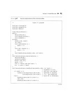
Code Fragment 13.15: Class Dijkstra implementing
Dijkstra's algorithm. (Continues in Code Fragment
13.16.)

850

The main computation of Dijkstra's algorithm is performed by method dijkstra
Visit. An adaptable priority queue Q supporting location-aware entries (Section
8.4.2) is used. We insert a vertex u into Q with method insert, which returns the
location-aware entry of u in Q. We "attach" to u its entry in Q by means of
method setEntry, and we retrieve the entry of u by means of method getEntry.

Note that associating entries to the vertices is an instance of the decorator design
pattern (Section 13.3.2). Instead of using an additional data structure for the labels
D[u], we exploit the fact that D[u] is the key of vertex u in Q, and thus D[u] can
be retrieved given the entry for u in Q. Changing the label of a vertex z to d in the
relaxation procedure corresponds to calling method replaceKey(e,d), where e is
the location-aware entry for z in Q.

851
Code Fragment 13.16: Method dijkstraVisit of class
Dijkstra . (Continued from Code Fragment 13.15
.)


852
13.7 Minimum Spanning Trees
Suppose we wish to connect all the computers in a new office building using the least
amount of cable. We can model this problem using a weighted graph G whose
vertices represent the computers, and whose edges represent all the possible pairs (u,
v) of computers, where the weight w((v, u)) of edge (v, u) is equal to the amount of
cable needed to connect computer v to computer u. Rather than computing a shortest
path tree from some particular vertex v, we are interested instead in finding a (free)
tree T that contains all the vertices of G and has the minimum total weight over all
such trees. Methods for finding such a tree are the focus of this section.
Problem Definition
Given a weighted undirected graph G, we are interested in finding a tree T that
contains all the vertices in G and minimizes the sum

A tree, such as this, that contains every vertex of a connected graph G is said to be a
spanning tree, and the problem of computing a spanning tree T with smallest total
weight is known as the minimum spanning tree (or MST) problem.

The development of efficient algorithms for the minimum spanning tree problem
predates the modern notion of computer science itself. In this section, we discuss
two classic algorithms for solving the MST problem. These algorithms are both
applications of the greedy method, which, as was discussed briefly in the previous
section, is based on choosing objects to join a growing collection by iteratively
picking an object that minimizes some cost function. The first algorithm we discuss
is Kruskal's algorithm, which "grows" the MST in clusters by considering edges in
order of their weights. The second algorithm we discuss is the Prim-Jarník
algorithm, which grows the MST from a single root vertex, much in the same way
as Dijkstra's shortest-path algorithm.
As in Section 13.6.1, in order to simplify the description of the algorithms, we
assume, in the following, that the input graph G is undirected (that is, all its edges
are undirected) and simple (that is, it has no self-loops and no parallel edges).
Hence, we denote the edges of G as unordered vertex pairs (u,z).
Before we discuss the details of these algorithms, however, let us give a crucial fact
about minimum spanning trees that forms the basis of the algorithms.
A Crucial Fact about Minimum Spanning Trees

853
The two MST algorithms we discuss are based on the greedy method, which in this
case depends crucially on the following fact. (See Figure 13.17.)
Figure 13.17: An illustration of the crucial fact about
minimum spanning trees.

Proposition 13.25: Let G be a weighted connected graph, and let V
1
and V
2

be a partition of the vertices of G into two disjoint nonempty sets. Furthermore, lete

be an edge in G with minimum weight from among those with one endpoint in V
1

and the other in V
2
. There is a minimum spanning tree T that has e as one of its
edges.
Justification: Let T be a minimum spanning tree of G. If T does not contain
edge e, the addition of e to T must create a cycle. Therefore, there is some edge f of
this cycle that has one endpoint in V
1
and the other in V
2
. Moreover, by the choice
of e, w(e) ≤ w(f). If we remove f from T { e}, we obtain a spanning tree whose total
weight is no more than before. Since T was a minimum spanning tree, this new tree
must also be a minimum spanning tree.

In fact, if the weights in G are distinct, then the minimum spanning tree is unique;
we leave the justification of this less crucial fact as an exercise (C-13.18)
. In
addition, note that Proposition 13.25 remains valid even if the graph G contains
negative-weight edges or negative-weight cycles, unlike the algorithms we
presented for shortest paths.

854