Ethernet Networks: Design, Implementation, Operation, Management 4th phần 6 doc
Bạn đang xem bản rút gọn của tài liệu. Xem và tải ngay bản đầy đủ của tài liệu tại đây (370.17 KB, 60 trang )
bridging and switching methods and performance issues 287
A
8
1
4
6
C
D
B
3
Figure 6.5 A weighted network graph.
Kruskal’s algorithm can be expressed as follows:
1. Sort the edges of the graph (G) in their increasing order by weight
or length.
2. Construct a subgraph (S) of G and initially set it to the empty state.
3. For each edge (e) in sorted order:
If the endpoints of the edges (e) are disconnected in S, add them to S.
Using the graph shown in Figure 6.5, let’s apply Kruskal’s algorithm
as follows:
1. The sorted edges of the graph in their increasing order by weight or
length produces the following table:
Edge
Weight/Length
A-C 1
B-D 3
C-B 4
C-D 6
A-B 8
2. Set the subgraph of G to the empty state. Thus, S = null.
3. For each edge add to S as long as the endpoints are disconnected. Thus,
the first operation produces:
A
C
S = A,C or
288 chapter six
The next operation produces:
A
S = (A,C) + (B,D) or
C
B
D
The third operation produces:
A
S = (A,B) + (B,D) + (C,B) or
C
B
D
Note that we cannot continue as the endpoints in S are now all connected.
Thus, the minimum spanning tree consists of the edges or links (A, B) +
(B, D) + (C, B) and has the weight 1 + 4 + 3, or 7. Now that we have an
appreciation for the method by which a minimum spanning tree is formed, let’s
turn our attention to its applicability in transparent bridge-based networks.
Similar to the root of a tree, one bridge in a spanning tree network will
be assigned to a unique position in the network. Known as the root bridge,
this bridge is assigned as the top of the spanning tree, and because of this
position, it has the potential to carry the largest amount of intranet traffic due
to its position.
Because bridges and bridge ports can be active or inactive, a mechanism
is required to identify bridges and bridge ports. Each bridge in a spanning
tree network is assigned a unique bridge identifier. This identifier is the MAC
address on the bridge’s lowest port number and a two-byte bridge priority
level. The priority level is defined when a bridge is installed and functions
as a bridge number. Similar to the bridge priority level, each adapter on
a bridge that functions as a port has a two-byte port identifier. Thus, the
unique bridge identifier and port identifier enable each port on a bridge to be
uniquely identified.
Path Cost
Under the spanning tree algorithm, the difference in physical routes between
bridges is recognized, and a mechanism is provided to indicate the preference
for one route over another. That mechanism is accomplished by the ability
bridging and switching methods and performance issues 289
to assign a path cost to each path. Thus, you could assign a low cost to a
preferred route and a high cost to a route you only want to be used in a
backup situation.
Once path costs are assigned to each path in an intranet, each bridge will
have one or more costs associated with different paths to the root bridge. One
of those costs is lower than all other path costs. That cost is known as the
bridge’s root path cost, and the port used to provide the least path cost toward
the root bridge is known as the root port.
Designated Bridge
As previously discussed, the spanning tree algorithm does not permit active
loops in an interconnected network. To prevent this situation from occurring,
only one bridge linking two networks can be in a forwarding state at any
particular time. That bridge is known as the designated bridge, while all other
bridges linking two networks will not forward frames and will be in a blocking
state of operation.
Constructing the Spanning Tree
The spanning tree algorithm employs a three-step process to develop an active
topology. F irst, the root bridge is identified. To accomplish this, each bridge
in the intranet will initially assume it is the root bridge. To determine which
bridge should actually act as the root bridge, each bridge will periodically
transmit bridge protocol data unit (BPDU) frames that are described in the
following section. BPDU frames under Ethernet version 2 are referred to as
HELLO frames or messages and are transmitted on all bridge ports. Each
BPDU frame includes the priority of the bridge defined at installation time. As
the bridges in the intranet periodically transmit their BPDU frames, bridges
receiving a BPDU with a lower priority value than its own cease transmitting
their BPDUs; however, they forward BPDUs with a lower priority value.
Thus, after a short period of time the bridge with the lowest priority value
is recognized as the root bridge. In Figure 6.3b we will assume bridge 1 was
selected as the root bridge. Next, the path cost from each bridge to the root
bridge is determined, and the minimum cost from each bridge becomes the
root path cost. The port in the direction of the least path cost to the root
bridge, known as the root port, is then determined for each bridge. If the root
path cost is the same for two or more bridges linking LANs, then the bridge
with the highest priority will be selected to furnish the minimum path cost.
Once the paths are selected, the designated ports are activated.
290 chapter six
In examining Figure 6.3a, let u s now use the cost entries assigned to
each bridge. Let us assume that bridge 1 was selected as the root bridge,
since we expect a large amount of traffic to flow between Token-Ring 1 and
Ethernet 1 networks. Therefore, bridge 1 will become the designated bridge
between Token-Ring 1 and Ethernet 1 networks. Here the term designated
bridge references the bridge that has the bridge port with the lowest-cost path
to the root bridge.
In examining the path costs to the root bridge, note that the path through
bridge 2 was assigned a cost of 10, while the path through bridge 3 was
assigned a cost of 15. Thus, the path from Token-Ring 2 via bridge 2 to Token-
Ring 1 becomes the designated bridge between those two networks. Hence,
Figure 6.3b shows bridge 3 inactive by the omission of a connection to the
Token-Ring 2 network. Similarly, the path cost for connecting the Ethernet 3
network to the root bridge is lower by routing through the Token-Ring 2 and
Token-Ring 1 networks. Thus, bridge 5 becomes the designated bridge for the
Ethernet 3 and Token-Ring 2 networks.
Bridge Protocol Data Unit
As previously noted, bridges obtain topology information by the use of
bridge protocol data unit (BPDU) frames. Once a root bridge is selected, that
bridge is responsible for periodically transmitting a ‘‘HELLO’’ BPDU frame
to all networks to which it is connected. According to the spanning tree
protocol, H ELLO frames must be transmitted every 1 to 10 seconds. The
BPDU has the group MAC address 800143000000, which is recognized by
each bridge. A designated bridge will then update the path cost and timing
information and forward the frame. A standby bridge will monitor the BPDUs,
but will not update nor forward them. If the designated bridge does not
receive a BPDU on its root port for a predefined period of time (default is
20 seconds), the designated bridge will assume that either a link or device
failure occurred. That bridge, if it is still receiving configuration BPDU frames
on other ports, will then switch its root port to a port that is receiving the best
configuration BPDUs.
When a standby bridge is required to assume the role of the root or designated
bridge, the HELLO BPDU will indicate that a standby bridge should become
a designated bridge. The process by which bridges determine their role in
a spanning tree network is iterative. As new bridges enter a network, they
assume a listening state to determine their role in the network. Similarly,
when a bridge is removed, another iterative process occurs to reconfigure the
remaining bridges.
bridging and switching methods and performance issues 291
Although the STP algorithm procedure eliminates duplicate frames and
degraded intranet performance, it can be a hindrance for situations where
multiple active paths between networks are desired. In addition, if a link or
device fails, the time required for a new spanning tree to be formed via the
transmission of BPDUs can easily require 45 to 60 seconds or more. Another
disadvantage of STP occurs when it is used in remote bridges connecting
geographically dispersed networks. For example, returning to Figure 6.2,
suppose Ethernet 1 were located in Los Angeles, E thernet 2 in New York, and
Ethernet 3 in Atlanta. If the link between Los Angeles and New York were
placed in a standby mode of operation, all frames from Ethernet 2 routed to
Ethernet 1 would be routed through Atlanta. Depending on the traffic between
networks, this situation might require an upgrade in the bandwidth of the links
connecting each network to accommodate the extra traffic flowing through
Atlanta. Since the yearly cost of upgrading a 56- or 64-Kbps circuit to a 128-
Kbps fractional T1 link can easily exceed the cost of a bridge or router, you
might wish to consider the use of routers to accommodate this networking
situation. In comparison, when using local bridges, the higher operating
rate of local bridges in interconnecting local area networks normally allows
an acceptable level of performance when LAN traffic is routed through an
intermediate bridge.
Protocol Dependency
Another problem associated with the use of transparent bridges concerns the
differences between Ethernet and IEEE 802.3 frame field compositions. As
noted in Chapter 4, the Ethernet frame contains a type field that indicates
the higher-layer protocol in use. Under the IEEE 802.3 frame format, the type
field is replaced by a length field, and the data field is subdivided to include
logical link control (LLC) information in the form of destination (DSAP) and
source (SSAP) service access points. Here, the DSAP and SSAP are similar to
the type field in an Ethernet frame: they also point to a higher-level process.
Unfortunately, this small difference can create problems when you are using
a transparent bridge to interconnect Ethernet and IEEE 802.3 networks.
The top portion of Figure 6.6 shows the use of a bridge to connect an
AppleTalk network supporting several Macintosh computers to an Ethernet
network on which a Digital Equipment Corporation VAX computer is located.
Although the VAX may be capable of supporting DecNet Phase IV, which
is true Ethernet, and AppleTalk if both modules are resident, a pointer is
required to direct the IEEE 802.3 frames generated by the Macintosh to
the right protocol on the VAX. Unfortunately, the Ethernet connection used
292 chapter six
Dec
phase IV
Apple
talk
Ethernet NIC
Ethernet
Ethernet
B
M
M
M
IEEE 802.3
IEEE 802.3
Length
InformationInformation
Information
DSAP
SSAP
Control
Type
Frame differences
Legend:
= Workstation
= Macintosh
Figure 6.6 Protocol differences preclude linking IEEE 802.3 and Ethernet
networks using transparent bridges. A Macintosh computer connected on an
IEEE 802.3 network using AppleTalk will not have its frame pointed to the
right process on a VAX on an Ethernet. Thus, the differences between Ethernet
and IEEE 802.3 networks require transparent bridges for interconnecting
similar networks.
by the VAX will not provide the required pointer. This explains why you
should avoid connecting Ethernet and IEEE 802.3 networks via transparent
bridges. Fortunately, almost all Ethernet NICs manufactured today are IEEE
802.3–compatible to alleviate this problem; however, older NICs may operate
as true Ethernets and result in the previously mentioned problem.
Source Routing
Source routing is a bridging technique developed by IBM for connecting
Token-Ring networks. The key to the implementation of source routing is the
bridging and switching methods and performance issues 293
use of a portion of the information field in the Token-Ring frame to carry
routing information and the transmission of discovery packets to d etermine
the best route between two networks.
The presence of source routing is indicated by the setting of the first bit
position in the source address field of a Token-Ring frame to a binary 1. When
set, this indicates that the information field is preceded by a route information
field (RIF), which contains both control and routing information.
The RIF Field
Figure 6.7 illustrates the composition of a Token-Ring RIF. This field is
variable in length and is developed during a discovery process, described
later in this section.
2 bytes
Up to 16 bytes
Control
Ring
#
Ring
#
Ring
#
Bridge
#
Bridge
#
Bridge
#
12 bits
4 bits
BBB
L
LL
L
L
LF LF
LF LF
RRRD
Field format
B are broadcast bits
Bit settings Designator
Bit settings
0XX
10X
11X
Nonbroadcast
All-routes broadcast
Single route broadcast
L are length bits which denote length of the RIF in bytes
D is direction bit
LF identifies largest frame
Size in bytes
000
001
010
011
100
101
110
111
516
1500
2052
4472
8191
Reserved
Reserved
Used in all-routes broadcast frame
R are reserved bits
Figure 6.7 Token-Ring route information field. The Token-Ring RIF is vari-
able in length.
294 chapter six
The control field contains information that defines how information will be
transferred and interpreted and what size the remainder of the RIF will be. The
three broadcast bit positions indicate a nonbroadcast, all-routes broadcast, or
single-route broadcast situation. A nonbroadcast designator indicates a local
or specific route frame. An all-routes broadcast d esignator indicates that a
frame will be transmitted along every route to the destination station. A
single-route broadcast designator is used only by designated bridges to relay
a frame from one network to another. In examining the broadcast bit settings
shown in Figure 6.7, note that the letter X indicates an unspecified bit setting
that can be either a 1 or 0.
The length bits identify the length of the RIF in bytes, while the D bit
indicates how the field is scanned, left to right or right to left. Since vendors
have incorporated different memory in bridges which may limit frame sizes,
the LF bits enable different devices to negotiate the size of the frame. Normally,
a default setting indicates a frame size of 512 bytes. Each bridge can select
a number, and if it is supported by other bridges, that number is then used
to represent the negotiated frame size. Otherwise, a smaller number used
to represent a smaller frame size is selected, and the negotiation process is
repeated. Note that a 1500-byte frame is the largest frame size supported
by Ethernet IEEE 802.3 networks. Thus, a bridge used to connect Ethernet
and Token-Ring networks cannot support the use of Token-Ring frames
exceeding 1500 bytes.
Up to eight route number subfields, each consisting of a 12-bit ring number
and a 4-bit bridge number, can be contained in the routing information field.
This permits two to eight route designators, enabling frames to traverse up
to eight rings across seven bridges in a given direction. Both ring numbers
and bridge numbers are expressed as hexadecimal characters, with three h ex
characters u sed to denote the ring number and one hex character used to
identify the bridge number.
Operation Example
To illustrate the concept behind source routing, consider the intranet illus-
trated in Figure 6.8. In this example, let us assume that two Token-Ring
networks are located in Atlanta and one network is located in New York.
Each Token-Ring and bridge is assigned a ring or bridge number. For sim-
plicity, ring numbers R1, R2, and R3 are used here, although as previously
explained, those numbers are actually represented in hexadecimal. Simi-
larly, bridge numbers are shown here as B1, B2, B3, B4, and B5 instead of
hexadecimal characters.
bridging and switching methods and performance issues 295
A
A
A
A
A
A
A
B
R1
R1
R1 R1
R1
R1
R1
B1
B2
B2
B1
B1
R3
R3
R3
0
0
C
D
B5
B5
R2
R2
R2
B4
B4
B4
R2
B3
B3
B3
B3
New York
Atlanta
Figure 6.8 Source routing discovery operation. The route discovery process
results in each bridge entering the originating ring number and its bridge
number into the RIF.
When a station wants to originate communications, it is responsible for
finding the destination by transmitting a discovery packet to network bridges
and other network stations whenever it has a message to transmit to a new
destination address. If station A wishes to transmit to station C, it sends a
route discovery packet containing an empty RIF and its source address, as
indicated in the upper left portion of Figure 6.8. This packet is recognized
by each source routing bridge in the network. When a source routing bridge
receives the packet, it enters the packet’s ring number and its own bridge
identifier in the packet’s routing information field. The bridge then transmits
the p acket to all of its connections except the connection on which the packet
was received, a process known as flooding. Depending on the topology of the
interconnected networks, it is more than likely that multiple copies of the
discovery packet will reach the recipient. This is illustrated in the upper right
corner of Figure 6.8, in which two discovery packets reach station C. Here, one
packet contains the sequence R1B1R1B2R30 — the zero indicates that there is
no bridging in the last ring. The second packet contains the route sequence
R1B3R2B4R2B5R30. Station C then picks the best route, based on either the
most direct path or the earliest arriving packet, and transmits a response to
296 chapter six
the discover packet originator. The response indicates the specific route to
use, and station A then enters that route into memory for the duration of the
transmission session.
Under source routing, bridges do not keep routing tables like transparent
bridges. Instead, tables are maintained at each station throughout the network.
Thus, each station must check its routing table to determine what route frames
must traverse to reach their destination station. This routing method results
in source routing using distributed routing tables instead of the centralized
routing tables used by transparent bridges.
Advantages
There are several advantages associated with source routing. One advantage is
the ability to construct mesh networks with loops for a fault-tolerant design;
this cannot be accomplished with the use of transparent bridges. Another
advantage is the inclusion of routing information in the information frames.
Several vendors have developed network management software products that
use that information to p rovide statistical information concerning intranet
activity. Those products may assist you in determining how heavily your
wide area network links are being used, and whether you need to modify the
capacity of those links; they may also inform you if one or more workstations
are hogging communications between networks.
Disadvantages
Although the preceding advantages are considerable, they are not without
a price. That price includes a requirement to identify bridges and links
specifically, higher bursts of network activity, and an incompatibility between
Token-Ring and Ethernet networks. In addition, because the structure of the
Token-Ring RIF supports a maximum of seven entries, routing of frames is
restricted to crossing a maximum of seven bridges.
When using source routing bridges to connect Token-Ring networks, you
must configure each bridge with a unique bridge/ring number. In addition,
unless you wish to accept the default method by which stations select a frame
during the route discovery process, you will have to reconfigure your LAN
software. Thus, source routing creates an administrative burden not incurred
by transparent bridges.
Due to the route discovery process, the flooding of discovery frames occurs in
bursts when stations are turned on or after a power outage. Depending upon
the complexity of an intranet, the discovery process can degrade network
bridging and switching methods and performance issues 297
performance. This is perhaps the most problematic for organizations that
require the interconnection of Ethernet and Token-Ring networks.
A source routing bridge can be used only to interconnect Token-Ring
networks, since it operates on RIF data not included in an Ethernet frame.
Although transparent bridges can operate in Ethernet, Token-Ring, and mixed
environments, their use precludes the ability to construct loop or mesh
topologies, and inhibits the ability to establish operational redundant paths
for load sharing. Another problem associated with bridging Ethernet and
Token-Ring networks involves the RIF in a Token-Ring frame. Unfortunately,
different LAN operating systems use the RIF data in different ways. Thus,
the use of a transparent bridge to interconnect Ethernet and Token-Ring
networks may require the same local area network operating system on each
network. To alleviate these problems, several vendors introduced source
routing transparent (SRT) bridges, which function in accordance with the
IEEE 802.1D standard approved during 1992.
Source Routing Transparent Bridges
A source routing transparent bridge supports both IBM’s source routing and
the IEEE transparent STP operations. This type of bridge can be considered
two bridges in one; it has been standardized by the IEEE 802.1 committee as
the IEEE 802.1D standard.
Operation
Under source routing, the MAC packets contain a status bit in the source field
that identifies whether source routing is to be used for a message. If source
routing is indicated, the bridge forwards the frame as a source routing frame. If
source routing is not indicated, the bridge determines the destination address
and processes the packet using a transparent mode of operation, using routing
tables generated by a spanning tree algorithm.
Advantages
There are several advantages associated with source routing transparent
bridges. First and perhaps foremost, they enable different networks to use
different local area network operating systems and protocols. This capabil-
ity enables you to interconnect networks developed independently of one
another, and allows organization departments and branches to use LAN
operating systems without restriction. Secondly, also a very important con-
sideration, source routing transparent bridges can connect Ethernet and
298 chapter six
Token-Ring networks while preserving the ability to mesh or loop Token-
Ring networks. Thus, their use provides an additional level of flexibility for
network construction.
Translating Operations
When interconnecting Ethernet/IEEE 802.3 and Token-Ring networks, the
difference between frame formats requires the conversion of frames. A bridge
that performs this conversion is referred to as a translating bridge.
As previously noted in Chapter 4, there are several types of Ethernet frames,
such as Ethernet, IEEE 802.3, Novell’s Ethernet-802.3, and Ethernet-SNAP.
The latter two frames represent variations of the physical IEEE 802.3 frame
format. Ethernet and Ethernet-802.3 do not use logical link control, while IEEE
802.3 CSMA/CD LANs specify the use of IEEE 802.2 logical link control. In
comparison, all IEEE 802.5 Token-Ring networks either directly or indirectly
use the IEEE 802.2 specification for logical link control.
The conversion from IEEE 802.3 to IEEE 802.5 can be accomplished by
discarding portions of the IEEE 802.3 frame not applicable to a Token-
Ring frame, copying the 802.2 LLC protocol data unit (PDU) from one
frame to another, and inserting fields applicable to the Token-Ring frame.
Figure 6.9 illustrates the conversion process performed by a translating bridge
Preamble
DA
DA
SA
SA
Length
DSAP
DSAP
SSAP
SSAP
Control
Control
Information
Information
FCS
FCS
Discard
insert
Discard
insert
Discard
insert
Copy
Copy
SD
AC
FC
RIF
ED
FS
Legend:
DA
SA
AC
FC
RIF
DSAP
SSAP
ED
FS
= Destination Address
= Source Address
= Access Control
= Frame Control
= Routing Information Field
= Destination Service Access Point
= Source Service Access Point
= End Delimiter
= Frame Status Field
IEEE 802.3
Figure 6.9 IEEE 802.3 to 802.5 frame conversion.
bridging and switching methods and performance issues 299
Preamble
DA
DA
SA
SA
DSAP
SSAP
Control
FCS
FCS
FCS
Discard
insert
Discard
insert
Copy
Copy
SD
AC
FC
RIF
ED
FS
Legend:
DA
SA
AC
FC
RIF
DSAP
SSAP
ED
FS
OC
= Destination Address
= Source Address
= Access Control
= Frame Control
= Routing Information Field
= Destination Service Access Point
= Source Service Access Point
= End Delimiter
= Frame Status Field
= Organization Code
Type
Type
Data
Data
OC
Ethernet
Token-
ring
Figure 6.10 Ethernet to Token-Ring frame conversion.
linking an IEEE 802.3 network to an IEEE 802.5 network. Note that fields
unique to the IEEE 802.3 frame are discarded, while fields common to both
frames are copied. Fields unique to the IEEE 802.5 frame are inserted by
the bridge.
Since an Ethernet frame, as well as Novell’s Ethernet-802.3 frame, does not
support logical link control, the conversion process to IEEE 802.5 requires
more processing. In addition, each conversion is more specific and may or
may not be supported by a specific translating bridge. For example, consider
the conversion of Ethernet frames to Token-Ring frames. Since Ethernet does
not support LLC PDUs, the translation process results in the generation of a
Token-Ring-SNAP frame. This conversion or translation process is illustrated
in Figure 6.10.
6.2 Bridge Network Utilization
In this section, we will examine the use of bridges to interconnect separate
local area networks and to subdivide networks to improve performance.
In addition, we will focus our attention on how we can increase network
300 chapter six
availability by employing bridges to provide alternate communications paths
between networks.
Serial and Sequential Bridging
The top of Figure 6.11 illustrates the basic use of a bridge to interconnect two
networks serially. Suppose that monitoring of each network indicates a high
level of intranetwork use. One possible configuration to reduce intra-LAN
traffic on each network can be obtained by moving some stations off each of
the two existing networks to form a third network. The three networks would
then be interconnected through the use of an additional bridge, as illustrated
in the middle portion of Figure 6.11. This extension results in sequential or
cascaded bridging, and is appropriate when intra-LAN traffic is necessary but
minimal. This intranet topology is also extremely useful when the length of an
Ethernet must be extended beyond the physical cabling of a single network. By
locating servers appropriately within each network segment, you may be able
to minimize inter-LAN transmission. For example, the first network segment
could be used to connect marketing personnel, while the second and third
segments could be used to connect engineering and personnel departments.
This might minimize the use of a server on one network by persons connected
to another network segment.
A word of caution is in order concerning the use of bridges. Bridging
formswhatisreferredtoasaflat network topology, because it makes its
forwarding decisions using layer 2 MAC addresses, which cannot distinguish
one network from another. This means that broadcast traffic generated on
one segment will be bridged onto other segments which, depending upon
the amount of broadcast traffic, can adversely affect the performance on
other segments.
The only way to reduce broadcast traffic between segments is to use a
filtering feature included with some bridges or install routers to link seg-
ments. Concerning the latter, routers operate at the network layer and forward
packets explicitly addressed to a different network. Through the use of net-
work addresses for forwarding decisions, routers form hierarchical structured
networks, eliminating the so-called broadcast storm effect that occurs when
broadcast traffic generated from different types of servers on different segments
are automatically forwarded by bridges onto other segments.
Both serial and sequential bridging are applicable to transparent, source
routing, and source routing transparent bridges that do not provide redun-
dancy nor the ability to balance traffic flowing between networks. Each of these
deficiencies can be alleviated through the use of parallel bridging. However,
bridging and switching methods and performance issues 301
B
B
B
B
B
Serial bridging
Sequential or cascaded bridging
Parallel bridging
Legend:
B
= Workstation
= Bridge
Figure 6.11 Serial, sequential, and parallel bridging.
this bridging technique creates a loop and is only applicable to source routing
and source routing transparent bridges.
Parallel Bridging
The lower portion of Figure 6.11 illustrates the use of p arallel bridges to
interconnect two Token-Ring networks. This bridging configuration permits
302 chapter six
one bridge to back up the other, providing a level of redundancy for linking
the two networks as well as a significant increase in the availability of one
network to communicate with another. For example, assume the availability
of each bridge used at the top of Figure 6.11 (serial bridging) and bottom
of Figure 6.11 (parallel bridging) is 90 percent. The availability through two
serially connected bridges would be 0.9 × 0.9 (availability of bridge 1 ×
availability of bridge 2), or 81 percent. In comparison, the availability through
parallel bridges would be 1 − (0.1 × 0.1), which is 99 percent.
The dual paths between networks also improve inter-LAN communications
performance, because communications between stations on each network can
be load balanced. The use of parallel bridges can thus be expected to provide a
higher level of inter-LAN communications than the use of serial or sequential
bridges. However, as previously noted, this topology is not supported by
transparent bridging.
Star Bridging
With a multiport bridge, you can connect three or more networks to form a
star intranet topology. The top portion of Figure 6.12 shows the use of one
bridge to form a star topology by interconnecting four separate networks.
This topology, or a variation on this topology, could be used to interconnect
networks on separate floors within a building. For example, the top network
could be on floor N + 1, while the bottom network could be on floor N − 1in
a building. The bridge and the two networks to the left and right of the bridge
might then be located on floor N.
Although star bridging permits several networks located on separate floors
within a building to be interconnected, all intranet data must flow through
one bridge. This can result in both performance and reliability constraints to
traffic flow. Thus, to interconnect separate networks on more than a few floors
in a building, you should consider using backbone bridging.
Backbone Bridging
The lower portion of Figure 6.12 illustrates the use of backbone bridging. In
this example, one network runs vertically through a building with Ethernet
ribs extending from the backbone onto each floor. Depending upon the amount
of intranet traffic and the vertical length required for the backbone network,
the backbone can be either a conventional Ethernet bus-based network or a
fiber-optic backbone.
bridging and switching methods and performance issues 303
Star bridging
Backbone bridging
B
B
B
B
B
Legend:
= Workstation
= Bridge
Figure 6.12 Star and backbone bridging.
6.3 Bridge Performance Issues
The key to obtaining an appropriate level of performance when intercon-
necting networks is planning. The actual planning process will depend upon
several factors, such as whether separate networks are in operation, the type
of networks to be connected, and the type of bridges to be used — local
or remote.
Traffic Flow
If separate networks are in operation and you have appropriate monitoring
equipment, you can determine the traffic flow on each of the networks to be
304 chapter six
interconnected. Once this is accomplished, you can expect an approximate
10- to 20-percent increase in network traffic. This additional traffic represents
the flow of information between networks after an interconnection links previ-
ously separated local area networks. Although this traffic increase represents
an average encountered by the author, your network traffic may not represent
the typical average. To explore further, you can examine the potential for
intranet communications in the form of electronic messages that may be trans-
mitted to users on other networks, potential file transfers of word processing
files, and other types of data that would flow between networks.
Network Types
The types of networks to be connected will govern the rate at which frames
are presented to bridges. This rate, in turn, will govern the filtering rate at
which bridges should operate so that they do not become bottlenecks on
a network. For example, the maximum number of frames per second will
vary between different types of Ethernet and Token-Ring networks, as well as
between different types of the same network. The operating rate of a bridge
may thus be appropriate for connecting some networks while inappropriate
for connecting other types of networks.
Type of Bridge
Last but not least, the type of bridge — local or remote — will have a con-
siderable bearing upon performance issues. Local bridges pass data between
networks at their operating rates. In comparison, remote bridges pass data
between networks using wide area network transmission facilities, which
typically provide a transmission rate that is only a fraction of a local area
network operating rate. Now that we have discussed some of the aspects
governing bridge and intranet performance using bridges, let’s probe deeper
by estimating network traffic.
Estimating Network Traffic
If we do not have access to monitoring equipment to analyze an existing
network, or if we are planning to install a new network, we can spend some
time developing a reasonable estimate of network traffic. To do so, we should
attempt to classify stations into groups based on the type of general activity
performed, and then estimate the network activity for one station per group.
This will enable us to multiply the number of stations in the group by the
bridging and switching methods and performance issues 305
station activity to determine the group network traffic. Adding up the activity
of all groups will then provide us with an estimate of the traffic activity for
the network.
As an example of local area network traffic estimation, let us assume that our
network will support 20 engineers, 5 managers, and 3 secretaries. Table 6.1
shows how we would estimate the network traffic in terms of the bit rate
for each station group and the total activity per group, and then sum up the
network traffic for the three groups that will use the network. In this example,
which for the sake of simplicity does not include the transmission of data to
a workstation printer, the total network traffic was estimated to be slightly
below 50,000 bps.
TABLE 6.1 Estimating Network Traffic
Activity
Message Size
(Bytes) Frequency Bit Rate
∗
Engineering workstations
Request program 1,500 1/hour 4
Load program 480,000 1/hour 1,067
Save files 120,000 2/hour 533
Send/receive e-mail 2,000 2/hour 9
Total engineering activity
= 1,613 × 20 = 32,260 bps 1,613
Managerial workstations
Request program 1,500 2/hour 7
Load program 320,000 2/hour 1,422
Save files 30,000 2/hour 134
Send/receive e-mail 3,000 4/hour 27
Total managerial activity
= 1,590 × 5 = 7,950 bps 1,590
Secretarial workstations
Request program 1,500 4/hour 14
Load program 640,000 2/hour 2,844
Save files 12,000 8/hour 214
Send/receive e-mail 3,000 6/hour 40
Total secretarial activity
= 3,112 × 3 = 9,336 bps 3,112
Total estimated network activity
= 49,546 bps
∗
Note: Bit rate is computed by multiplying message rate by frequency by 8 bits/byte and dividing
by 3,600 seconds/hour.
306 chapter six
To plan for the interconnection of two or more networks through the use
of bridges, our next step should be to perform a similar traffic analysis for
each of the remaining networks. After this is accomplished, we can use the
network traffic to estimate inter-LAN traffic, using 10 to 20 percent of total
intranetwork traffic as an estimate of the intranet traffic that will result from
the connection of separate networks.
Intranet Traffic
To illustrate the traffic estimation process for the interconnection of separate
LANs, let us assume that network A’s traffic was determined to be 50,000 bps,
while network B’s traffic was estimated to be approximately 100,000 bps.
Figure 6.13 illustrates the flow of data between networks connected by a local
bridge. Note that the data flow in each direction is expressed as a range, based
on the use of an industry average of 10 to 20 percent of network traffic routed
between interconnected networks.
Network Types
Our next area of concern is to examine the types of networks to be intercon-
nected. In doing so, we should focus our attention on the operating rate of
Network A
Local traffic
50,000 bps
Network B
Local traffic
100,000 bps
10,000 to 20,000 bps
B
Total traffic 60,000 to 70,000 bps
Total traffic 105,000 to 110,000 bps
5,000 to 10,000 bps
Legend:
= Workstation
Figure 6.13 Considering intranet data flow. To determine the traffic flow on
separate networks after they are interconnected, you must consider the flow
of data onto each network from the other network.
bridging and switching methods and performance issues 307
each LAN. If network A’s traffic was estimated to be approximately 50,000 bps,
then the addition of 10,000 to 20,000 bps from network B onto network A will
raise network A’s traffic level to between 60,000 and 70,000 bps. Similarly,
the addition of traffic from network A onto network B will raise network B’s
traffic level to between 105,000 and 110,000 bps. In this example, the resulting
traffic on each network is well below the operating rate of all types of local
area networks, and will not present a capacity problem for either network.
Bridge Type
As previously mentioned, local bridges transmit data between networks at
the data rate of the destination network. This means that a local bridge will
have a lower probability of being a bottleneck than a remote bridge, since the
latter provides a connection between networks using a wide area transmission
facility, which typically operates at a fraction of the operating r ate of a LAN.
In examining the bridge operating rate required to connect networks, we
will use a bottom-up and a top-down approach. That is, we will first determine
the operating rate in frames per second for the specific example previously
discussed. This will be followed by computing the maximum frame rate
supported by an Ethernet network.
For the bridge illustrated in Figure 6.13, we previously computed that its
maximum transfer rate would be 20,000 bps from network B onto network A.
This is equivalent to 2500 bytes per second. If we assume that data is trans-
ported in 512-byte frames, this would be equivalent to 6 frames per second — a
minimal transfer rate supported by every bridge manufacturer. However, when
remote bridges are used, the frame forwarding rate of the bridge will more
than likely be constrained by the operating rate of the wide area network
transmission facility.
Bridge Operational Considerations
A remote bridge wraps a LAN frame into a higher-level protocol packet
for transmission over a wide area network communications facility. This
operation requires the addition of a header, protocol control, error detection,
and trailer fields, and results in a degree of overhead. A 20,000-bps data flow
from network B to network A, therefore, could not be accommodated by a
transmission facility operating at that data rate.
In converting LAN traffic onto a wide area network transmission facility,
you can expect a protocol overhead of approximately 20 percent. Thus, your
actual operating rate must be at least 24,000 bps before the wide area network
communications link becomes a bottleneck and degrades communications.
308 chapter six
Now that we have examined the bridging performance requirements for two
relatively small networks, let us focus our attention on determining the
maximum frame rates of an Ethernet network. This will provide us with the
ability to determine the rate at which the frame processing rate of a bridge
becomes irrelevant, since any processing rate above the maximum network
rate will not be useful. In addition, we can use the maximum network
frame rate when estimating traffic, because if we approach that rate, network
performance will begin to degrade significantly when use exceeds between 60
to 70 percent of that rate.
Ethernet Traffic Estimation
An Ethernet frame can vary between a minimum of 72 bytes and a maximum
of 1526 bytes. Thus, the maximum frame rate on an Ethernet will vary with
the frame size.
Ethernet operations require a dead time between frames of 9.6 µsec. The bit
time for a 10-Mbps Ethernet is 1/10
7
or 100 nsec. Based upon the preceding,
we can compute the maximum number of frames/second for 1526-byte frames.
Here, the time per frame becomes:
9.6 µsec + 1526 bytes × 8 bits/byte
or 9.6 µsec + 12,208 bits × 100 nsec/bit
or 1.23 msec
Thus, in one second there can be a maximum of 1/1.23 msec or 812 maximum-
size frames. For a minimum frame size of 72 bytes, the time per frame is:
9.6 µsec + 72 bytes × 8 bits/byte × 100 nsec/bit
or 67.2 × 10
−6
sec.
Thus, in one second there can be a maximum of 1/67.2 × 10
−6
or 14,880
minimum-size 72-byte frames. Since 100BASE-T Fast Ethernet uses the same
frame composition as Ethernet, the maximum frame rate for maximum- and
minimum-length frames are ten times that of Ethernet. That is, Fast Ethernet
supports a maximum of 8120 maximum-size 1526-byte frames per second
and a maximum of 148,800 minimum-size 72-byte frames per second. Sim-
ilarly, Gigabit Ethernet uses the same frame composition as Ethernet but is
100 times faster. This means that Gigabit Ethernet is capable of support-
ing a maximum of 81,200 maximum-length 1526-byte frames per second
bridging and switching methods and performance issues 309
and a maximum of 1,488,000 minimum-length 72-byte frames per second.
As you might expect, 10 Gigabit Ethernet expands support by an order of
magnitude beyond the frame rate of Gigabit Ethernet. For both Gigabit and
10 Gigabit Ethernet the maximum frame rates are for full-duplex operations.
Table 6.2 summarizes the frame processing requirements for a 10-Mbps Ether-
net, Fast Ethernet, Gigabit Ethernet, and 10 Gigabit Ethernet under 50 percent
and 100 percent load conditions, based on minimum and maximum frame
lengths. Note that those frame processing requirements define the frame exam-
ination (filtering) operating rate of a bridge connected to different types of
Ethernet networks. That rate indicates the number of frames per second a
bridge connected to different types of Ethernet local area networks must be
capable of examining under heavy (50-percent load) and full (100-percent
load) traffic conditions.
In examining the different E thernet network frame processing requirements
indicated in Table 6.2, it is important to note that the frame processing require-
ments associated with Fast Ethernet, Gigabit Ethernet, and 10 Gigabit Ethernet
commonly preclude the ability to upgrade a bridge by simply changing its
adapter cards. Due to the much greater frame processing requirements associ-
ated with very high speed Ethernet networks, bridges are commonly designed
to support those technologies from the ground up to include adapters and a
TABLE 6.2 Ethernet Frame Processing Requirements
(Frames per Second)
Frame Processing Requirements
Average Frame Size (Bytes) 50% Load 100% Load
Ethernet
1526 406 812
72 7440 14,880
Fast Ethernet
1526 4050 8120
72 74,400 148,800
Gigabit Ethernet
1526 40,600 81,200
72 744,000 1,488,000
10 Gigabit Ethernet
1526 406,000 812,000
72 7,440,000 14,880,000
310 chapter six
central processor to support the additional frame processing associated with
their higher operating rate.
We can extend our analysis of Ethernet frames by considering the frame
rate supported by different link speeds. For example, let us consider a pair of
remote bridges connected by a 9.6-Kbps line. The time per frame for a 72-byte
frame at 9.6 Kbps is:
9.6 × 10
−6
+ 72 × 8 × 0.0001041 s/bit or 0.0599712 seconds per frame
Thus, in one second the number of frames is 1/.0599712, or 16.67 frames per
second. Table 6.3 compares the frame-per-second rate supported by different
link speeds for minimum- and maximum-size Ethernet frames. As expected,
the frame transmission rate supported by a 10-Mbps link for minimum- and
maximum-size frames is exactly the same as the frame processing requirements
under 100 percent loading for a 10-Mbps Ethernet LAN, as indicated in
Table 6.2.
In examining Table 6.3, note that the entries in this table do not consider
the effect of the overhead of a protocol used to transport frames between
two networks. You should therefore decrease the frame-per-second rate by
approximately 20 percent for all link speeds through 1.536 Mbps. The reason
the 10-Mbps rate should not be adjusted is that it represents a local 10-
Mbps Ethernet bridge connection that does not require the use of a wide
area network protocol to transport frames. Also note that the link speed of
1.536 Mbps represents a T1 transmission facility that operates at 1.544 Mbps.
However, since the framing bits on a T1 circuit use 8 Kbps, the effective line
speed available for the transmission of data is 1.536 Mbps.
TABLE 6.3 Link Speed versus Frame Rate
Frames per Second
Link Speed Minimum Maximum
9.6 Kbps 16.67 0.79
19.2 Kbps 33.38 1.58
56.0 Kbps 97.44 4.60
64.0 Kbps 111.17 5.25
1.536 Mbps 2815.31 136.34
10.0 Mbps 14,880.00 812.00
bridging and switching methods and performance issues 311
Predicting Throughput
Until now, we have assumed that the operating rate of each LAN linked
by a bridge is the same. However, in many organizations this may not
be true, because LANs are implemented at different times using different
technologies. Thus, accounting may be using a 10-Mbps LAN, while the
personnel department might be using a 100-Mbps LAN.
Suppose we wanted to interconnect the two LANs via the use of a multi-
media bridge. To predict throughput between LANs, let us use the network
configuration illustrated in Figure 6.14. Here, the operating rate of LAN A is
assumed to be R
1
bps, while the operating rate of LAN B is assumed to be
R
2
bps.
In one second, R
1
bits can be transferred on LAN A and R
2
bits can be
transferred on LAN B. Similarly, it takes 1/R
1
seconds to transfer one bit on
LAN A and 1/R
2
seconds to transfer one bit on LAN B. So, to transfer one
bit across the bridge from LAN A to LAN B, ignoring the transfer time at
the bridge:
1
R
T
=
1
R
1
+
1
R
2
or
R
T
=
1
(1/R
1
) + (1/R
2
)
We computed that a 10-Mbps Ethernet would support a maximum transfer of
812 maximum-sized frames per second. If we assume that the second LAN
operating at 100 Mbps is also an Ethernet, we would compute its transfer rate
to be approximately 8120 maximum-sized frames per second. The throughput
in frames per second would then become:
R
T
=
1
(1/812) + (1/8120)
= 738 frames per second
Knowing the transfer rate between LANs can help us answer many common
questions. It can also provide us with a mechanism for determining whether
LAN A
LAN B
R
1
R
2
Bridge
Figure 6.14 Linking LANs with different operating rates. When LANs with
different operating rates (R
1
and R
2
) are connected via a bridge, access of files
across the bridge may result in an unacceptable level of performance.