INTRODUCTION TO KNOWLEDGE DISCOVERY AND DATA MINING - CHAPTER 3 pot
Bạn đang xem bản rút gọn của tài liệu. Xem và tải ngay bản đầy đủ của tài liệu tại đây (379.5 KB, 15 trang )
33
Chapter 3
Data Mining with Decision Trees
Decision trees are powerful and popular tools for classification and prediction. The
attractiveness of tree-based methods is due in large part to the fact that, in contrast to
neural networks, decision trees represent rules. Rules can readily be expressed so
that we humans can understand them or in a database access language like SQL so
that records falling into a particular category may be retrieved.
In some applications, the accuracy of a classification or prediction is the only thing
that matters; if a direct mail firm obtains a model that can accurately predict which
members of a prospect pool are most likely to respond to a certain solicitation, they
may not care how or why the model works. In other situations, the ability to explain
the reason for a decision is crucial. In health insurance underwriting, for example,
there are legal prohibitions against discrimination based on certain variables. An in-
surance company could find itself in the position of having to demonstrate to the sat-
isfaction of a court of law that it has not used illegal discriminatory practices in
granting or denying coverage. There are a variety of algorithms for building decision
trees that share the desirable trait of explicability. Most notably are two methods and
systems CART and C4.5 (See5/C5.0) that are gaining popularity and are now avail-
able as commercial software.
3.1 How a decision tree works
Decision tree is a classifier in the form of a tree structure where each node is either:
a leaf node, indicating a class of instances, or
a decision node that specifies some test to be carried out on a single attribute
value, with one branch and sub-tree for each possible outcome of the test.
A decision tree can be used to classify an instance by starting at the root of the tree
and moving through it until a leaf node, which provides the classification of the in-
stance.
Example: Decision making in the London stock market
Suppose that the major factors affecting the London stock market are:
what it did yesterday;
what the New York market is doing today;
bank interest rate;
Knowledge Discovery and Data Mining
34
unemployment rate;
England’s prospect at cricket.
Table 3.1 is a small illustrative dataset of six days about the London stock market.
The lower part contains data of each day according to five questions, and the second
row shows the observed result (Yes (Y) or No (N) for “It rises today”). Figure 3.1 il-
lustrates a typical learned decision tree from the data in Table 3.1.
Instance No.
It rises today
1
Y
2
Y
3
Y
4
N
5
N
6
N
It rose yesterday
NY rises today
Bank rate high
Unemployment high
England is losing
Y
Y
N
N
Y
Y
N
Y
Y
Y
N
N
N
Y
Y
Y
N
Y
N
Y
N
N
N
N
Y
N
N
Y
N
Y
Table 3.1: Examples of a small dataset on the London stock market
is unemployment high?
YES NO
The London market
will rise today {2,3}
is the New York market
rising today?
YES NO
The London market
will rise today {1}
The London market
will not rise today {4, 5, 6}
Figure 3.1: A decision tree for the London stock market
The process of predicting an instance by this decision tree can also be expressed by
answering the questions in the following order:
Is unemployment high?
YES: The London market will rise today
NO: Is the New York market rising today?
YES: The London market will rise today
NO: The London market will not rise today.
35
Decision tree induction is a typical inductive approach to learn knowledge on classi-
fication. The key requirements to do mining with decision trees are:
Attribute-value description: object or case must be expressible in terms of a
fixed collection of properties or attributes.
Predefined classes: The categories to which cases are to be assigned must
have been established beforehand (supervised data).
Discrete classes: A case does or does not belong to a particular class, and
there must be for more cases than classes.
Sufficient data: Usually hundreds or even thousands of training cases.
“Logical” classification model: Classifier that can be only expressed as deci-
sion trees or set of production rules
3.2 Constructing decision trees
3.2.1 The basic decision tree learning algorithm
Most algorithms that have been developed for learning decision trees are variations
on a core algorithm that employs a top-down, greedy search through the space of
possible decision trees. Decision tree programs construct a decision tree T from a set
of training cases. The original idea of construction of decision trees goes back to the
work of Hoveland and Hunt on concept learning systems (CLS) in the late 1950s.
Table 3.2 briefly describes this CLS scheme that is in fact a recursive top-down di-
vide-and-conquer algorithm. The algorithm consists of five steps.
1. T the whole training set. Create a T node.
2. If all examples in T are positive, create a ‘P’ node with T as its parent and
stop.
3. If all examples in T are negative, create a ‘N’ node with T as its parent and
stop.
4. Select an attribute X with values v
1
, v
2
, …, v
N
and partition T into subsets T
1
,
T
2
, …, T
N
according their values on X. Create N nodes T
i
(i = 1, , N) with T
as their parent and X = v
i
as the label of the branch from T to T
i
.
5. For each T
i
do: T T
i
and goto step 2.
Table 3.2: CLS algorithm
We present here the basic algorithm for decision tree learning, corresponding ap-
proximately to the ID3 algorithm of Quinlan, and its successors C4.5, See5/C5.0 [12].
To illustrate the operation of ID3, consider the learning task represented by training
examples of Table 3.3. Here the target attribute PlayTennis (also called class attrib-
ute), which can have values yes or no for different Saturday mornings, is to be pre-
dicted based on other attributes of the morning in question.
Knowledge Discovery and Data Mining
36
Day Outlook Temperature Humidity Wind PlayTennis?
D1
D2
D3
D4
D5
D6
D7
D8
D9
D10
D11
D12
D13
D14
Sunny
Sunny
Overcast
Rain
Rain
Rain
Overcast
Sunny
Sunny
Rain
Sunny
Overcast
Overcast
Rain
Hot
Hot
Hot
Mild
Cool
Cool
Cool
Mild
Cool
Mild
Mild
Mild
Hot
Mild
High
High
High
High
Normal
Normal
Normal
High
Normal
Normal
Normal
High
Normal
High
Weak
Strong
Weak
Weak
Weak
Strong
Strong
Weak
Weak
Weak
Strong
Strong
Weak
Strong
No
No
Yes
Yes
Yes
No
Yes
No
Yes
Yes
Yes
Yes
Yes
No
Table 3.3: Training examples for the target concept PlayTennis
3.2.1 Which attribute is the best classifier?
The central choice in the ID3 algorithm is selecting which attribute to test at each
node in the tree, according to the first task in step 4 of the CLS algorithm. We would
like to select the attribute that is most useful for classifying examples. What is a good
quantitative measure of the worth of an attribute? We will define a statistical prop-
erty called information gain that measures how well a given attribute separates the
training examples according to their target classification. ID3 uses this information
gain measure to select among the candidate attributes at each step while growing the
tree.
Entropy measures homogeneity of examples. In order to define information gain
precisely, we begin by defining a measure commonly used in information theory,
called entropy, that characterizes the (im)purity of an arbitrary collection of exam-
ples. Given a collection S, containing positive and negative examples of some target
concept, the entropy of S relative to this Boolean classification is
Entropy(S) = - p
⊕
log
2
p
⊕
- p
⊖
log
2
p
⊖
(3.1)
where p
⊕
is the proportion of positive examples in S and p
⊖
is the proportion of nega-
tive examples in S. In all calculations involving entropy we define 0log0 to be 0.
To illustrate, suppose S is a collection of 14 examples of some Boolean concept, in-
cluding 9 positive and 5 negative examples (we adopt the notation [9+, 5-] to sum-
marize such a sample of data). Then the entropy of S relative to this Boolean classifi-
cation is
37
Entropy([9+, 5-]) = - (9/14) log
2
(9/14) - (5/14) log
2
(5/14) = 0.940 (3.2)
Notice that the entropy is 0 if all members of S belong to the same class. For exam-
ple, if all members are positive (p
⊕
= 1 ), then p
⊖
is 0, and Entropy(S) = -1 log
2
(1) -
0log
2
0 = -10 - 0log
2
0 = 0. Note the entropy is 1 when the collection contains an
equal number of positive and negative examples. If the collection contains unequal
numbers of positive and negative examples, the entropy is between 0 and 1. Figure
3.1 shows the form of the entropy function relative to a Boolean classification, as p
⊕
varies between 0 and 1.
Figure 3.1: The entropy function relative to a Boolean classification, as the propor-
tion of positive examples p
⊕
varies between 0 and 1.
One interpretation of entropy from information theory is that it specifies the mini-
mum number of bits of information needed to encode the classification of an arbi-
trary member of S (i.e., a member of S drawn at random with uniform probability).
For example, if p
⊕
is 1, the receiver knows the drawn example will be positive, so no
message need be sent, and the entropy is 0. On the other hand, if p
⊕
is 0.5, one bit is
required to indicate whether the drawn example is positive or negative. If p
⊕
is 0.8,
then a collection of messages can be encoded using on average less than 1 bit per
message by assigning shorter codes to collections of positive examples and longer
codes to less likely negative examples.
Thus far we have discussed entropy in the special case where the target classification
is Boolean. More generally, if the target attribute can take on c different values, then
the entropy of S relative to this c-wise classification is defined as
log)(
2
1
i
c
i
i
ppSEntropy
(3.3)
where p
i
is the proportion of S belonging to class i. Note the logarithm is still base 2
because entropy is a measure of the expected encoding length measured in bits. Note
Knowledge Discovery and Data Mining
38
also that if the target attribute can take on c possible values, the entropy can be as
large as log
2
c.
Information gain measures the expected reduction in entropy. Given entropy as a
measure of the impurity in a collection of training examples, we can now define a
measure of the effectiveness of an attribute in classifying the training data. The
measure we will use, called information gain, is simply the expected reduction in en-
tropy caused by partitioning the examples according to this attribute. More precisely,
the information gain, Gain (S, A) of an attribute A, relative to a collection of exam-
ples S, is defined as
)(
||
||
)(),(
)(
v
AValuesv
v
SEntropy
S
S
SEntropyASGain
(3.4)
where Values(A) is the set of all possible values for attribute A, and S
v
is the subset of
S for which attribute A has value v (i.e., S
v
= {s ∊ S |A(s) = v}). Note the first term in
Equation (3.4) is just the entropy of the original collection S and the second term is
the expected value of the entropy after S is partitioned using attribute A. The ex-
pected entropy described by this second term is simply the sum of the entropies of
each subset S
v
, weighted by the fraction of examples |S
v
|/|S| that belong to S
v
. Gain
(S,A) is therefore the expected reduction in entropy caused by knowing the value of
attribute A. Put another way, Gain(S,A) is the information provided about the target
function value, given the value of some other attribute A. The value of Gain(S,A) is
the number of bits saved when encoding the target value of an arbitrary member of S,
by knowing the value of attribute A.
For example, suppose S is a collection of training-example days described in Table
3.3 by attributes including Wind, which can have the values Weak or Strong. As be-
fore, assume S is a collection containing 14 examples ([9+, 5-]). Of these 14 exam-
ples, 6 of the positive and 2 of the negative examples have Wind = Weak, and the
remainder have Wind = Strong. The information gain due to sorting the original 14
examples by the attribute Wind may then be calculated as
0.048
(6/14)1.00- 1(8/14)0.81 - 0.940
)()14/6()(8/14) -
)(
||
||
)(),(
]3,3[
]2,6[
,5-][9
, )(
},{
StrongWeak
v
StrongWeakv
v
Strong
Weak
SEntropyEntropy(SEntropy(S)
SEntropy
S
S
SEntropyWindSGain
S
S
S
StrongWeakWindValues
39
Information gain is precisely the measure used by ID3 to select the best attribute at
each step in growing the tree.
An Illustrative Example. Consider the first step through the algorithm, in which the
topmost node of the decision tree is created. Which attribute should be tested first in
the tree? ID3 determines the information gain for each candidate attribute (i.e., Out-
look, Temperature, Humidity, and Wind), then selects the one with highest informa-
tion gain. The information gain values for all four attributes are
Gain(S, Outlook) = 0.246
Gain(S, Humidity) = 0.151
Gain(S, Wind) = 0.048
Gain(S, Temperature) = 0.029
where S denotes the collection of training examples from Table 3.3.
According to the information gain measure, the Outlook attribute provides the best
prediction of the target attribute, PlayTennis, over the training examples. Therefore,
Outlook is selected as the decision attribute for the root node, and branches are cre-
ated below the root for each of its possible values (i.e., Sunny, Overcast, and Rain).
The final tree is shown in Figure 3.2.
Outlook
Humidity Wind
Sunny Overcast Rain
No Yes No Yes
High Normal Strong Weak
Yes
Figure 3.2. A decision tree for the concept PlayTennis
The process of selecting a new attribute and partitioning the training examples is now
repeated for each non-terminal descendant node, this time using only the training ex-
amples associated with that node. Attributes that have been incorporated higher in
the tree are excluded, so that any given attribute can appear at most once along any
path through the tree. This process continues for each new leaf node until either of
two conditions is met:
1. every attribute has already been included along this path through the tree, or
2. the training examples associated with this leaf node all have the same target
attribute value (i.e., their entropy is zero).
Knowledge Discovery and Data Mining
40
3.3 Issues in data mining with decision trees
Practical issues in learning decision trees include determining how deeply to grow
the decision tree, handling continuous attributes, choosing an appropriate attribute
selection measure, handling training data with missing attribute values, handing at-
tributes with differing costs, and improving computational efficiency. Below we dis-
cuss each of these issues and extensions to the basic ID3 algorithm that address them.
ID3 has itself been extended to address most of these issues, with the resulting sys-
tem renamed C4.5 and See5/C5.0 [12].
3.3.1 Avoiding over-fitting the data
The CLS algorithm described in Table 3.2 grows each branch of the tree just deeply
enough to perfectly classify the training examples. While this is sometimes a reason-
able strategy, in fact it can lead to difficulties when there is noise in the data, or when
the number of training examples is too small to produce a representative sample of
the true target function. In either of these cases, this simple algorithm can produce
trees that over-fit the training examples.
Over-fitting is a significant practical difficulty for decision tree learning and many
other learning methods. For example, in one experimental study of ID3 involving
five different learning tasks with noisy, non-deterministic data, over-fitting was
found to decrease the accuracy of learned decision trees by l0-25% on most problems.
There are several approaches to avoiding over-fitting in decision tree learning. These
can be grouped into two classes:
approaches that stop growing the tree earlier, before it reaches the point
where it perfectly classifies the training data,
approaches that allow the tree to over-fit the data, and then post prune the tree.
Although the first of these approaches might seem more direct, the second approach
of post-pruning over-fit trees has been found to be more successful in practice. This
is due to the difficulty in the first approach of estimating precisely when to stop
growing the tree.
Regardless of whether the correct tree size is found by stopping early or by post-
pruning, a key question is what criterion is to be used to determine the correct final
tree size. Approaches include:
Use a separate set of examples, distinct from the training examples, to evalu-
ate the utility of post-pruning nodes from the tree.
41
Use all the available data for training, but apply a statistical test to estimate
whether expanding (or pruning) a particular node is likely to produce an im-
provement beyond the training set. For example, Quinlan [12] uses a chi-
square test to estimate whether further expanding a node is likely to improve
performance over the entire instance distribution, or only on the current sam-
ple of training data.
Use an explicit measure of the complexity for encoding the training examples
and the decision tree, halting growth of the tree when this encoding size is
minimized. This approach, based on a heuristic called the Minimum Descrip-
tion Length principle.
The first of the above approaches is the most common and is often referred to as a
training and validation set approach. We discuss the two main variants of this ap-
proach below. In this approach, the available data are separated into two sets of ex-
amples: a training set, which is used to form the learned hypothesis, and a separate
validation set, which is used to evaluate the accuracy of this hypothesis over subse-
quent data and, in particular, to evaluate the impact of pruning this hypothesis.
Reduced error pruning. How exactly might we use a validation set to prevent over-
fitting? One approach, called reduced-error pruning (Quinlan, 1987), is to consider
each of the decision nodes in the tree to be candidates for pruning. Pruning a decision
node consists of removing the sub-tree rooted at that node, making it a leaf node, and
assigning it the most common classification of the training examples affiliated with
that node. Nodes are removed only if the resulting pruned tree performs no worse
than the original over the validation set. This has the effect that any leaf node added
due to coincidental regularities in the training set is likely to be pruned because these
same coincidences are unlikely to occur in the validation set. Nodes are pruned itera-
tively, always choosing the node whose removal most increases the decision tree ac-
curacy over the validation set. Pruning of nodes continues until further pruning is
harmful (i.e., decreases accuracy of the tree over the validation set).
3.3.2 Rule post-pruning
In practice, one quite successful method for finding high accuracy hypotheses is a
technique we shall call rule post-pruning. A variant of this pruning method is used by
C4.5 [15]4]. Rule post-pruning involves the following steps:
1. Infer the decision tree from the training set, growing the tree until the training
data is fit as well as possible and allowing over-fitting to occur.
2. Convert the learned tree into an equivalent set of rules by creating one rule
for each path from the root node to a leaf node.
3. Prune (generalize) each rule by removing any preconditions that result in im-
proving its estimated accuracy.
4. Sort the pruned rules by their estimated accuracy, and consider them in this
sequence when classifying subsequent instances.
Knowledge Discovery and Data Mining
42
To illustrate, consider again the decision tree in Figure 3.2. In rule post-pruning, one
rule is generated for each leaf node in the tree. Each attribute test along the path from
the root to the leaf becomes a rule antecedent (precondition) and the classification at
the leaf node becomes the rule consequent (post-condition). For example, the left-
most path of the tree in Figure 3.2 is translated into the rule
IF (Outlook = Sunny) ∧ (Humidity = High)
THEN PlayTennis = No
Next, each such rule is pruned by removing any antecedent, or precondition, whose
removal does not worsen its estimated accuracy. Given the above rule, for example,
rule post-pruning would consider removing the preconditions (Outlook = Sunny) and
(Humidity = High). It would select whichever of these pruning steps produced the
greatest improvement in estimated rule accuracy, then consider pruning the second
precondition as a further pruning step. No pruning step is performed if it reduces the
estimated rule accuracy.
Why convert the decision tree to rules before pruning? There are three main advan-
tages.
Converting to rules allows distinguishing among the different contexts in
which a decision node is used. Because each distinct path through the deci-
sion tree node produces a distinct rule, the pruning decision regarding that at-
tribute test can be made differently for each path. In contrast, if the tree itself
were pruned, the only two choices would be to remove the decision node
completely, or to retain it in its original form.
Converting to rules removes the distinction between attribute tests that occur
near the root of the tree and those that occur near the leaves. Thus, we avoid
messy bookkeeping issues such as how to reorganize the tree if the root node
is pruned while retaining part of the sub-tree below this test.
Converting to rules improves readability. Rules are often easier for people to
understand.
3.3.3 Incorporating Continuous-Valued Attributes
The initial definition of ID3 is restricted to attributes that take on a discrete set of
values. First, the target attribute whose value is predicted by the learned tree must be
discrete valued. Second, the attributes tested in the decision nodes of the tree must
also be discrete valued. This second restriction can easily be removed so that con-
tinuous-valued decision attributes can be incorporated into the learned tree. This can
be accomplished by dynamically defining new discrete-valued attributes that parti-
tion the continuous attribute value into a discrete set of intervals. In particular, for an
attribute A that is continuous-valued, the algorithm can dynamically create a new
Boolean attribute A
c
that is true if A < c and false otherwise. The only question is
how to select the best value for the threshold c. As an example, suppose we wish to
include the continuous-valued attribute Temperature in describing the training exam-
43
ple days in Table 3.3. Suppose further that the training examples associated with a
particular node in the decision tree have the following values for Temperature and
the target attribute PlayTennis.
Temperature: 40 48 60 72 80 90
PlayTennis: No No Yes Yes Yes No
What threshold-based Boolean attribute should be defined based on Temperature?
Clearly, we would like to pick a threshold, c, that produces the greatest information
gain. By sorting the examples according to the continuous attribute A, then identify-
ing adjacent examples that differ in their target classification, we can generate a set
of candidate thresholds midway between the corresponding values of A. It can be
shown that the value of c that maximizes information gain must always lie at such a
boundary. These candidate thresholds can then be evaluated by computing the infor-
mation gain associated with each. In the current example, there are two candidate
thresholds, corresponding to the values of Temperature at which the value of Play-
Tennis changes: (48 + 60)/2 and (80 + 90)/2. The information gain can then be com-
puted for each of the candidate attributes, Temperature>54 and Temperature>85, and
the best can t selected (Temperature>54). This dynamically created Boolean attribute
can then compete with the other discrete-valued candidate attributes available for
growing the decision tree.
3.3.4 Handling Training Examples with Missing Attribute Values
In certain cases, the available data may be missing values for some attributes. For
example, in a medical domain in which we wish to predict patient outcome based on
various laboratory tests, it may be that the lab test Blood-Test-Result is available
only for a subset of the patients. In such cases, it is common to estimate the missing
attribute value based on other examples for which this attribute has a known value.
Consider the situation in which Gain(S, A) is to be calculated at node n in the deci-
sion tree to evaluate whether the attribute A is the best attribute to test at this decision
node. Suppose that <x, c(x)> is one of the training examples in S and that the value
A(x) is unknown, where c(x) is the class label of x.
One strategy for dealing with the missing attribute value is to assign it the value that
is most common among training examples at node n. Alternatively, we might assign
it the most common value among examples at node n that have the classification c(x).
The elaborated training example using this estimated value for A(x) can then be used
directly by the existing decision tree learning algorithm.
A second, more complex procedure is to assign a probability to each of the possible
values of A rather than simply assigning the most common value to A(x). These
probabilities can be estimated again based on the observed frequencies of the various
values for A among the examples at node n. For example, given a Boolean attribute A,
if node n contains six known examples with A = 1 and four with A = 0, then we
Knowledge Discovery and Data Mining
44
would say the probability that A(x) = 1 is 0.6, and the probability that A(x) = 0 is 0.4.
A fractional 0.6 of instance x is now distributed down the branch for A = 1 and a
fractional 0.4 of x down the other tree branch. These fractional examples are used for
the purpose of computing information Gain and can be further subdivided at subse-
quent branches of the tree if a second missing attribute value must be tested. This
same fractioning of examples can also be applied after learning, to classify new in-
stances whose attribute values are unknown. In this case, the classification of the new
instance is simply the most probable classification, computed by summing the
weights of the instance fragments classified in different ways at the leaf nodes of the
tree. This method for handling missing attribute values is used in C4.5.
3.4 Visualization of decision trees in system CABRO
In this section we briefly describe system CABRO for mining decision trees that fo-
cuses on visualization and model selection techniques in decision tree learning [11].
Though decision trees are a simple notion it is not easy to understand and analyze
large decision trees generated from huge data sets. For example, the widely used pro-
gram C4.5 produces a decision tree of nearly 18,500 nodes with 2624 leaf nodes from
the census bureau database given recently to the KDD community that consists of
199,523 instances described by 40 numeric and symbolic attributes (103 Mbytes). It
is extremely difficult for the user to understand and use that big tree in its text form.
In such cases, a graphic visualization of discovered decision trees with different ways
of accessing and viewing trees is of great support and recently it receives much atten-
tion from the KDD researcher and user. System MineSet of Silicon Graphics provides
a 3D visualization of decision trees. System CART (Salfort Systems) provides a tree
map that can be used to navigate the large decision trees. The interactive visualization
system CABRO, associated with a new proposed technique called T2.5D (stands for
Tree 2.5 Dimensions) offers an alternative efficient way that allows the user to ma-
nipulate graphically and interactively large trees in data mining.
In CABRO, a mining process concerns with model selection in which the user try dif-
ferent settings of decision tree induction to attain most appropriate decision trees. To
help the user to understand the effects of settings on result trees, the tree visualizer is
capable of handling multiple views of different trees at any stage in the induction.
There are several modes of view: zoomed, tiny, tightly-coupled, fish-eyed, and T2.5D,
in each mode the user can interactively change the layout of the structure to fit the
current interests.
The tree visualizer helps the user to understand decision trees by providing different
views; each is convenient to use in different situations. The available views are
45
Standard: The tree is drawn in proportion, the size of a node is up to the
length of its label, a father is vertically located at the middle of its children,
and sibling are horizontally aligned.
Tightly-coupled: The window is divided into two panels, one displays the tree
in a tiny size, another displays it in a normal size. The first panel is a map to
navigate the tree, the second displays the corresponding area of the tree.
Fish-eyes: This view distorts the magnified image so that nodes around the
center of interest is displayed at high magnification, and the rest of the tree is
progressively compressed.
T2.5D: In this view, Z-order of tree nodes are used to make an 3D effects,
nodes and links may be overlapped. The focused path of the tree is drawn in
the front and by highlighted colors.
The tree visualizer allows the user to customize above views by several operations
that include: zoom, collapse/expand, and view node content.
Zoom: The user can zoom in or zoom out the drawn tree.
Collapse/expand: The user can choose to view some parts of the tree by col-
lapsing and expanding paths.
View node content: The user can see the content of a node such as: attrib-
ute/value, class, population, etc.
In model selection, the tree visualization has an important role in assisting the user to
understand and interpret generated decision trees. Without its help, the user cannot
decide to favor which decision trees more than the others. Moreover, if the mining
process is set to run interactively, the system allows the user to be able to take part at
every step of the induction. He/she can manually choose which attribute will be used
to branch at the considering node. The tree visualizer then can display several hypo-
thetical decision trees side by side to help user to decide which ones are worth to fur-
ther develop. We can say that an interactive tree visualizer integrated with the system
allows the user to use domain knowledge by actively taking part in mining processes.
Very large hierarchical structures are still difficult to navigate and view even with
tightly-coupled and fish-eye views. To address the problem, we have been developing
a special technique called T2.5D (Tree 2.5 Dimensions). The 3D browsers usually can
display more nodes in a compact area of the screen but require currently expensive
3D animation support and visualized structures are difficult to navigate, while 2D
browsers have limitation in display many nodes in one view. The T2.5D technique
combines the advantages of both 2D and 3D drawing techniques to provides the user
with cheap processing cost a browser which can display more than 1000 nodes in one
view; a large number of them may be partially overlapped but they all are in full size.
In T2.5D, a node can be highlighted or dim. The highlighted nodes are that the user
currently interested in and they are displayed in 2D to be viewed and navigated with
ease. The dim nodes are displayed in 3D and they allow the user to get an idea about
overall structure of the hierarchy (Figure 3.3).
Knowledge Discovery and Data Mining
46
Figure 3.3. T2.5 Visualization of large decision trees
3.5 Strengths and Weakness of Decision Tree Methods
3.5.1 The strengths of decision tree methods
The strengths of decision tree methods are:
Decision trees are able to generate understandable rules.
Decision trees perform classification without requiring much computation.
Decision trees are able to handle both continuous and categorical variables.
Decision trees provide a clear indication of which fields are most important
for prediction or classification.
Ability to Generate Understandable Rules. The ability of decision trees to generate
rules that can be translated into comprehensible English or SQL is the greatest
strength of this technique. Even when a complex domain or a domain that does de-
compose easily into rectangular regions causes the decision tree to be large and com-
plex, it is generally fairly easy to follow any one path through the tree. So the expla-
nation for any particular classification or prediction is relatively straightforward.
Ability to Perform in Rule-Oriented Domains. It may sound obvious, but rule in-
duction in general, and decision trees in particular, are an excellent choice in do-
mains where there really are rules to be found. The authors had this fact driven home
to them by an experience at Caterpillar. Caterpillar called upon MRJ to help design
and oversee some experiments in data mining. One of the areas where we felt that
data mining might prove useful was in the automatic approval of warranty repair
claims. Many domains, ranging from genetics to industrial processes really do have
underlying rules, though these may be quite complex and obscured by noisy data.
47
Decision trees are a natural choice when you suspect the existence of underlying
rules.
Ease of Calculation at Classification Time. Although, as we have seen, a decision
tree can take many forms, in practice, the algorithms used to produce decision trees
generally yield trees with a low branching factor and simple tests at each node. Typi-
cal tests include numeric comparisons, set membership, and simple conjunctions.
When implemented on a computer, these tests translate into simple Boolean and in-
teger operations that are fast and inexpensive. This is an important point because in a
commercial environment, a predictive model is likely to be used to classify many
millions or even billions of records.
Ability to Handle Both Continuous and Categorical Variables. Decision-tree
methods are equally adept at handling continuous and categorical variables. Cate-
gorical variables, which pose problems for neural networks and statistical techniques,
come ready-made with their own splitting criteria: one branch for each category.
Continuous variables are equally easy to split by picking a number somewhere in
their range of values.
Ability to Clearly Indicate Best Fields. Decision-tree building algorithms put the
field that does the best job of splitting the training records at the root node of the tree.
3.5.2 The weaknesses of decision tree methods
Decision trees are less appropriate for estimation tasks where the goal is to predict
the value of a continuous variable such as income, blood pressure, or interest rate.
Decision trees are also problematic for time-series data unless a lot of effort is put
into presenting the data in such a way that trends and sequential patterns are made
visible.
Error-Prone with Too Many Classes. Some decision-tree algorithms can only deal
with binary-valued target classes (yes/no, accept/reject). Others are able to assign re-
cords to an arbitrary number of classes, but are error-prone when the number of train-
ing examples per class gets small. This can happen rather quickly in a tree with many
levels and/or many branches per node.
Computationally Expensive to Train. The process of growing a decision tree is
computationally expensive. At each node, each candidate splitting field must be
sorted before its best split can be found. In some algorithms, combinations of fields
are used and a search must be made for optimal combining weights. Pruning algo-
rithms can also be expensive since many candidate sub-trees must be formed and
compared.
Trouble with Non-Rectangular Regions. Most decision-tree algorithms only exam-
ine a single field at a time. This leads to rectangular classification boxes that may not
correspond well with the actual distribution of records in the decision space.