MANAGEMENT DYNAMICS Merging Constraints Accounting to Drive Improvement phần 5 ppsx
Bạn đang xem bản rút gọn của tài liệu. Xem và tải ngay bản đầy đủ của tài liệu tại đây (427.98 KB, 33 trang )
EXPLOITATION DECISIONS
In this section we explore the ways in which the global T, I, and OE mea-
surements affect exploitation decisions as we use the measurements to
guide decision making within a constraints accounting framework. Ex-
ploitation decisions that are supported by cost analysis, such as production
batch sizing, throughput (or sales) mix, and pricing, are influenced by
constraints accounting measurement in similar ways. The setup cost com-
ponent of the production batch-sizing model and throughput mix are
considered in this chapter, and the pricing question is considered in the
next.
Exploitation has to do with getting the most throughput out of the
existing environment. The significant constraints accounting attribute in
the financial analyses for exploitation is the explicit recognition of the
throughput effect of opportunity costs. The major financial impact will al-
ways be in terms of potentially expanded or lost throughput. If the analysis
does not reveal a significant throughput effect, then it points to a
choopchick.
41
Setup Cost
Consider the case of setup cost, which is a component of the traditional
batch-sizing model. The traditional model is illustrated in Exhibit 5.13.
The cost of setting up equipment consists of the labor and materials
costs, with the labor cost portion likely comprising the major portion. As
the quantity of units produced with each setup (which is the production
batch size) increases, the total annual setup cost and average setup cost
per unit decrease. Larger batch sizes imply fewer batches and less cost.
Exploitation Decisions 115
Exhibit 5.13 Traditional Batch Size Model
$-
$10
$20
$30
$40
$50
$60
$70
1 3 5 7 9 11 13 15 17 19
Setup Cost
Batch Size
Total Costs
Carrying Cost
Total Cost
5070_Pages 7/14/04 1:55 PM Page 115
The traditional perspective of setup cost is shown in Exhibit 5.13 and sub-
sequent exhibits by the “square” line.
Consider an example with the following characteristics:
• Annual carrying cost: $ 3 per unit
• Annual sales: $ 10,000,000
• Annual raw materials usage: $ 6,000,000
• Setup time for a resource: 2 hours
• Materials consumed in setup: $ 0
• Labor and labor-related costs: $ 30 per hour
• Annual resource time available: 2,000 hours
The traditional calculation of the setup cost for this resource would
be calculated as shown in Exhibit 5.14.
The $60 per setup is the amount represented by the “square” line for
the traditional analysis in Exhibit 5.13.
Reexamine the model of Exhibit 5.13 with reference to constraints
accounting. If the resource being set up is not a capacity-constrained re-
source and labor is essentially fixed, then reducing the number of setups
or time required for an individual setup on the resource will have no ef-
fect on labor costs. Only when the setup involves destruction of expensive
materials would the costs behave as the traditional model assumes. The
constraints accounting analysis of the setup cost for a nonconstraint re-
source is shown in Exhibit 5.15.
The nonconstraint resource setup cost would actually plot as the
horizontal line traced by the “diamonds” in Exhibit 5.16. Thus, setup time
reductions on nonconstraint resources will be, at best, choopchicks.
If the resource is an internal physical constraint, however, then setup
time is actually production time lost to the entire chain of events. Here
the opportunity cost of the lost throughput to the entire chain provides
the appropriate relationship to profitability. The opportunity cost may in-
clude current sales that are turned away because of lack of capacity or fu-
ture sales that are not made when current customers who do not receive
timely deliveries seek out alternate suppliers. In the case of a constraint re-
source, the traditional model considerably understates the impact of re-
116 Constraints Accounting Terminology and Technique
Exhibit 5.14 Cost of Setup: Traditional Analysis
(setup time x
x
labor rate) +
+
materials used
=
Setup cost
(2 hr / setup $30 / hr) $0
=
$60 / setup
5070_Pages 7/14/04 1:55 PM Page 116
ducing the setup time or number of setups. A constraints accounting
analysis of setup cost for the constrained resource based on current sales
turned away is shown in Exhibit 5.17.
The constrained resource curve is shown in Exhibit 5.18. The con-
strained resource curve is dramatically steeper and starts at a radically
higher point than the traditional analysis. The traditional analysis curve
shown in Exhibits 5.13 and 5.16 is repeated in Exhibit 5.18 for purposes of
comparison. It will be found at the bottom of the graph, very close to the
horizontal axis. Recognition that the throughput effect, as reflected in op-
portunity cost, defines the nature of relevant costs for a constrained re-
source leads to a different perception of the situation.
When viewed through the lens of constraints accounting, the tradi-
tional analysis of setup costs is faulty in every case. For unconstrained areas,
the cost is slightly overstated, and the effect is similar to that previously ob-
served in scenarios 1 and 4 of the thinking bridges example (Chapter 1)
and summarized in Exhibit 1.22, which is repeated here as Exhibit 5.19.
For activities holding an internal physical constraint, the financial
impact of the traditional analysis, which relies on historical cost, is signifi-
cantly understated in a manner similar to scenarios 2 and 3 of Exhibit
Exploitation Decisions 117
Exhibit 5.15 Cost of Setup: Constraints Accounting Analysis—
Nonconstraint Resource
Change in total labor and materials cost due to setup = Setup cost
$0 = $ 0 / setup
Exhibit 5.16 Setup Costs: Traditional and Nonconstraint Analyses
$-
$40
$50
$60
$70
1 5 9 13 17
Traditional
Batch size
Total Costs
Nonconstraint
5070_Pages 7/14/04 1:55 PM Page 117
5.19. Similar limitations apply to the financial analyses supporting other
operating decisions.
Throughput Mix
An organization may sell a variety of products and services comprising sev-
eral product lines in an assortment of geographical market areas. The or-
ganization may have multiple methods of distribution and various classes
of customer. The relative contributions of these individual elements to the
total throughput of the organization is referred to collectively as the
throughput mix.
118 Constraints Accounting Terminology and Technique
Exhibit 5.18 Setup Costs: Traditional and Constrained Resource Analysis
$-
$1,000
$2,000
$3,000
$4,000
$5,000
1
3
5
7
9
11
13
15
17
19
Traditional
Batch Size
Total Costs
Constrained
Resource
Exhibit 5.17 Cost of Setup: Constraints Accounting Analysis, Constrained
Resource
Annual sales $10,000,000
Annual raw materials usage 6,000,000
Annual throughput (T) $ 4,000,000
T/Constraint time available = O
=
pportunity cost of constraint hour
($4,000,000/yr) / (2,000 hours/yr) $2,000 / hour
(setup time) x (opportunity cost) Setup cost
2 hours / setup x $2,000 / hour =
=
$4,000 / setup
5070_Pages 7/14/04 1:55 PM Page 118
Throughput Mix with Production Constraint
When there is an internal physical constraint in the production area, the
company does not have sufficient internal capacity to satisfy all of the de-
mand for its products or services. In this case, decisions must be made
about what products to sell in which markets and to which customers.
Let us use an example to study the decision process for this case.
Some production data for the Example Company are presented in Exhibit
5.20.
42
The Example Company currently has the capability to produce three
products—Atex, Detron, and Fonic. As shown in Exhibit 5.20, the market
potential (i.e., the maximum amount that could be sold with the current
pricing and market conditions) is 2,080 units of Atex, 4,160 units of De-
tron, and 2,080 units of Fonic per year. Atex requires raw materials costing
$65 for each unit produced and comprised of material ARM, which has a
standard cost of $30, and raw material CRM, which costs $35. In similar
fashion, Detron’s raw materials cost $95 and Fonic’s are $65.
The raw materials are processed through a number of operations in-
volving welding, cutting, polishing, grinding, and assembly. Atex does not
require the welding operation, and Fonic does not go through assembly.
The process and setup times required for each product are shown in Ex-
hibit 5.20. From this data it is apparent that the welder is an internal phys-
Exploitation Decisions 119
Exhibit 5.19 Example Summary: First Year Dollar Gain or (Loss) Shown
by Analyses
Least Product
Cost
(LPC)
T, I, & OE
(TIOE)
Which analytical
technique do you
believe more correctly
reflects reality?
Scenario 1 $17,085 ($ 5,000)
Scenario 2 $ 26,500 ($ 123,400)
Scenario 3 ($36,500) $133,880
Scenario 4 $ 26,500 ($ 5,000)
Range of
Estimates of
Bottom-line
Profit Effect
$63,000 $257,280
5070_Pages 7/14/04 1:55 PM Page 119
ical constraint. A total of 170,560 minutes of process time in the welding
operation would be required to satisfy the entire market potential for the
three products. However, only 124,800 minutes of welding time are avail-
able for the year.
43
Not all of the potential quantities demanded can be
satisfied, and it will be necessary to decide what products to sell.
Sales and operational expense data for the Example Company are
provided in Exhibit 5.21.
The average unit sales prices for Atex and Detron are $175 and
$275, respectively. The budgeted operational expense, inclusive of manu-
facturing overhead, direct labor, sales and marketing, and general admin-
120 Constraints Accounting Terminology and Technique
Exhibit 5.20 Example Company: Production Data
Atex Detron Fonic
Market potential (units) 2,080 4,160 2,080
Raw materials used and cost:
ARM $ 30.00
$
30.00
CRM 35.00 35.00
ERM 30.00
FRM $ 65.00
Materials cost per unit $ 65.00 $ 95.00 $ 65.00
Direct labor and process time (minutes):
Annual resource minutes
Tota l
available
Needed to
meet potential
* Welder 0 34.000 14.000 124,800 *170,560
Cutter 24.000 9.000 15.000 249,600 118,560
Polisher 33.000 14.000 22.000 249,600 172,640
Grinder 20.000 18.000 27.000 249,600 172,640
Assembler 8.000
17.000 0 124,800 87,360
Direct labor minutes per unit 85.000 92.000 78.000
* Internal constraint
Setup time required per production batch (minutes):
Welder 0 30.000 15.000
Cutter 360.000 240.000 120.000
Polisher 120.000 120.000 120.000
Grinder 30.000 30.000 60.000
Assembler 0
0 0
Setup time per batch 510.000 420.000 315.000
Setup minutes per unit
(batch size = 20 units) 25.500 21.000 15.750
Direct labor: 8 employees earning $10.00 per hour and working 2,080 hours per year.
5070_Pages 7/14/04 1:55 PM Page 120
istrative expense, is $671,200 per year. The company uses a production
overhead rate of 200% of direct labor cost, calculated by dividing the bud-
geted manufacturing overhead of $332,800 by $166,400 of budgeted di-
rect labor cost.
Budgeted sales are 2,080 units of Atex, 3,515 units of Detron, and no
Fonic. Both Detron and Fonic require use of the constrained welding re-
source. In making the decision to emphasize Detron over Fonic, the com-
pany first calculated the product cost using absorption costing as shown in
Exhibit 5.22.
Exploitation Decisions 121
Exhibit 5.21 Example Company: Sales and Operational Expense (OE)
Data
Atex Detron Fonic
Current sales mix (units) 2,080 3,515 0
Unit sales price (current) $ 175.00 $ 275.00 $ 180.00
Sales commissions 5% of sales 5% of sales 5% of sales
Budgeted annual operational expense (OE):
Manufacturing overhead $ 332,800
Direct labor 166,400
Sales and marketing 72,000
General and administrative 100,000
Total budgeted operational expense (OE) $ 671,200
Production overhead rate: $332,800 / $166,400 = 200% of direct labor cost
Exhibit 5.22 Product Unit Cost Summary (Absorption Costing)
Traditional Unit Cost Summary
Atex
Detron Fonic
Materials cost $ 65.000 $ 95.000 $ 65.000
Setup labor @ $10.00 per hour 4.250 3.500 2.625
Factory overhead @ 200% of
setup labor 8.500 7.000 5.250
Direct labor @ $10.00 per hour 14.167 15.333 13.000
Factory overhead @ 200% of
direct labor 28.333
30.667 26.000
Total unit cost $120.250 $151.500 $111.875
5070_Pages 7/14/04 1:55 PM Page 121
The unit costs were then used to rank the products in terms of their
gross margin. This ranking is reflected in Exhibit 5.23.
Detron was ranked first, with the largest gross margin at 45%, fol-
lowed by Fonic at 38%, and Atex at 31%.
Being aware of the limitations of traditional absorption costing for
decision making, the company also checked the contribution margins. As
shown in Exhibit 5.24, the ranking remained the same.
The company used the gross margin ranking, as confirmed by the
contribution margin analysis, to guide it in its decision to use the welding
capacity to produce as much Detron as possible and turn any remaining
welding capacity to the production of Fonic. Since each unit of Detron re-
quired 34 minutes of welding process time plus 1.5 minutes of setup
time,
44
or a total 35.5 minutes, the company can produce 3,515 units of
Detron.
45
Because the potential market is 4,160 units, the Detron con-
sumes the entire welding capacity and no Fonic is produced. This results
122 Constraints Accounting Terminology and Technique
Exhibit 5.23 Gross Margin Analysis
Atex Detron Fonic
Unit selling price $ 175.00 $ 275.00 $ 180.00
Unit cost 120.25 151.50 111.87
Gross margin per unit $ 54.75 $ 123.50 $ 68.13
Gross margin as % of sales 31% 45% 38%
Rank in terms of
profitability 3 1 2
Exhibit 5.24 Contribution Margin Analysis
Atex Detron Fonic
Unit selling price $ 175.00 $ 275.00 $ 180.00
Variable expense:
Materials $ 65.00 $ 95.00 $ 65.00
Sales commissions at 5% 8.75
___13.75 9.00
Total variable expense $ 73.75 $ 108.75 $ 74.00
Contribution margin per unit (t) $ 101.25 $ 166.25 $ 106.00
Contribution margin as percent of
sales 58%
3
61% 59%
Rank in terms of profitability 1 2
5070_Pages 7/14/04 1:55 PM Page 122
in a budgeted profit of $123,769 as shown in Exhibit 5.25. In general,
management is pleased with this outcome.
The foregoing analysis is flawed from a constraints accounting point
of view. It fails to correctly incorporate into the decision the first two at-
tributes of constraints accounting—explicit consideration of the role of
constraints and specification of throughput contribution effects. Let us
look closely at the decision process steps that were followed:
• It was determined that the market potential was greater than the
company’s ability to supply it; that is, there is an internal con-
straint in the system.
• The potential products were ranked in terms of profitability using
the unit gross margin and/or throughput contribution margin
(either in dollars or percentages).
• The rankings were used to determine how much of each product
would be offered to the market while remaining within the physi-
cal capabilities of the company.
That is, preference decision (ranking the products by profitability)
was made without explicit consideration of the constraint and failed to consider the
impact of the constraint on throughput. Only the question of how much to
produce, given a previous preference decision, addressed the constraint.
The constraints accounting analysis illustrated in Exhibit 5.26 incor-
porates the explicit recognition of the throughput contribution effects of
the constraint.
Exploitation Decisions 123
Exhibit 5.25 Budgeted Profit Emphasizing Detron over Fonic
Budgeted Earnings Statement
Original Forecast—Emphasizing Detron over Fonic
Throughput
(unit contribution margins (t) from Exhibit 5.23)
Detron (3,515 units @ $166.25) 584,369
Atex (2,080 units @ $101.25) 210,600
$ 794,969
Operational expense
Direct labor $ 166,400
$
Manufacturing overhead 332,800
Sales and marketing 72,000
General and administrative 100,000
671,200
Net Profit $ 123,769
5070_Pages 7/14/04 1:55 PM Page 123
The constraints accounting analysis ranks the products in the oppo-
site order. Atex appears to be the most profitable in terms of the welding
constraint. Since Atex does not require use of the welder, its return is infi-
nite in terms of welder time. Fonic returns half again as much throughput
for each welder minute used as does Detron. The constraints accounting
preference decision, then, is to make all 2,080 units of Atex and as much
Fonic as is possible and can be sold, turning any remaining welder capac-
ity to the production of Detron. Since each unit of Fonic requires about
14 minutes for processing and an average of 45 seconds for setup, the Ex-
ample Company can produce all 2,080 units of the market potential for
Fonic in 30,680 minutes (14.75 minutes per unit * 2,080 units). That will
leave 94,120 minutes on the welder for Detron, during which 2,651 units
of Detron may be produced (94,120 minutes divided by 35.5 minutes per
unit). The budgeted result of this revised throughput mix is shown in Ex-
hibit 5.27.
The updated forecast of Exhibit 5.27 reveals an increase in budgeted
net profit of $76,840 from $123,769 to $200,609, or an increase of 62% re-
sulting from the revised throughput mix.
Beyond Product Throughput
The throughput per constraint unit, when calculated for each product,
does not tell the entire story. For example, the sales to individual cus-
tomers might be as shown in Exhibit 5.28.
Inspection of Exhibit 5.28 shows that the Example Company would
prefer to sell Detron to customer 02, with a throughput per constraint
unit (t/cu) of $6.36, than Fonic to customer 05, which has a t/cu of $5.85.
The company would also want to consider that customer 05 accounts for
124 Constraints Accounting Terminology and Technique
Exhibit 5.26 Constraints Accounting Analysis
Atex Detron Fonic
Unit selling price $ 175.00 $ 275.00 $ 180.00
Variable expense:
Materials $ 65.00 $ 95.00 $ 65.00
Sales commissions at 5.00% 8.75
13.75 9.00
Total variable expense $ 73.75 $ 108.75 $ 74.00
Throughput contribution (t) per unit
$ 101.25
$ 166.25 $ 106.00
Physical constraint minutes per unit 0 3
1
414
Throughput value of product in terms
of constraint minute (t/cu)
infinite 4.89 $ 7.57
Rank in terms of profitability 3 2
5070_Pages 7/14/04 1:55 PM Page 124
almost half of the total throughput. They should also estimate the effect
that reducing sales of Fonic to customer 05 might have on other sales to
customer 05.
Finally, the Example Company would ensure that its tactical exploita-
tion decisions were consistent with the strategic exploitation decisions em-
bodied in the organization’s strategic plan.
46
For example, assume that the
Exploitation Decisions 125
Exhibit 5.28 Sales by Customer
Customer Product Quantity Price Throughput
Throughput per
constraint unit (t/cu*)
Customer
t/cu*
Cust 01 Atex 416 $ 180.00 $ 44,096
Detron 530 $ 322.86 112,210 $5.96
Fonic 416 $ 180.71 44,377 $ 7.23 $8.04
Cust 02 Atex 270 $ 189.05 30,941
Detron 162 $ 337.65 36,574 $6.36
Fonic 241 $ 211.00 32,643 $9.18 $10.76
Cust 03 Atex 36 9 $ 180.96 39,451
Detron 4 8 $ 256.14 7,120 $4.18
Fonic 109 $ 208.07 14,461 $8.99 $18.43
Cust 04 Atex 145 $ 194.16 17,321
Detron 80 $ 209.57 8,327 $ 2.93
Fonic 599 $ 186.67 67,290 $ 7.62 $7.96
Cust 05 Atex 880 $ 162.6 7 78,792
Detron 1,831 $ 258.9 6 276,497 $4.25
Fonic 715 $ 159.27 61,710
$5.85 $ 5.52
Total $871,810
* Constraint unit (cu) is welder minutes.
Exhibit 5.27 Budgeted Profit Emphasizing Fonic over Detron
Budgeted Earnings Statement
Updated Forecast—Emphasizing Fonic over Detron
Throughput
(unit contribution margins (t) from Exhibit 5.25)
Atex (2,080 units @ $101.25) $ 210,600
Detron (2,651 units @ $166.25) 440,729
Fonic (2,080 units @ $106.00) 220,480
$ 871,809
Operational expense
Direct labor $ 166,400
Factory overhead 332,800
Sales and marketing 72,000
General and administrative 100,000
671,200
Net Profit $ 200,609
5070_Pages 7/14/04 1:55 PM Page 125
126 Constraints Accounting Terminology and Technique
Example Company had determined, for whatever reasons, that it desired
to have the cutter become the constraint. That is, the cutter has been des-
ignated as the strategic constraint. Detron makes better use of the cutter, in
terms of throughput per cutter minute,
47
than does either Fonic or Atex.
The calculations are shown in Exhibit 5.29.
Management will need to assess the potential damage that would re-
sult from shifting production from Detron to Fonic. In the short run,
$76,840 is to be gained from throughput opportunity revisions (the differ-
ence between the budgeted net profits shown in Exhibits 5.25 and 5.27).
The conflict may be set out in the form of an evaporating cloud as shown
in Exhibit 5.30.
The objective of the cloud (A) is to increase the value of the com-
pany.
48
In order to increase the company’s present value, we must (B) ex-
ploit the current tactical constraint, which is the welder. In order to ex-
ploit the current tactical constraint, we must (D) use the constraint to
produce the higher t/cu product (emphasize Fonic over Detron). How-
ever, in order to (A) increase the value of the company, we must (C) sub-
ordinate to the exploitation decisions for the strategic plan, which is to
have the cutter become the constraint. In order to subordinate to the ex-
ploitation decisions for the strategic plan, we must (E) produce products
that will make the best use of the strategic constraint (emphasize Detron
over Fonic). Emphasizing Fonic over Detron is in conflict with emphasiz-
ing Detron over Fonic.
The assumptions that underlie each of the arrows should be
checked. For example, the D to E conflict arrow assumes that the produc-
tion capability is limited to the existing internal capacity. If outsourcing
some of the welding for either Fonic or Detron were a possibility, this as-
sumption would be invalid and the conflict would not exist. In similar
fashion, an assumption underlying the linkage between C and E is that the
company will lose the future market for Detron if the current market for
Detron is not also served. This may or may not be a valid assumption.
Exhibit 5.29 Throughput per Cutter Minute
Atex Detron Fonic
Average throughput per unit (Exhibit 5.26) $101.25 $166.25 $106.00
Cutter time required for processing and
setup for one unit
42
minutes
21 minutes 21 minutes
Throughput (t) per cutter minute $2.41 $7.92 $5.05
Rank if cutter were to become a constraint 3 1 2
5070_Pages 7/14/04 1:55 PM Page 126
Throughput Mix with Marketing Constraint
As important as it is to consider throughput stated in terms of an internal
physical constraint, we must also know when a measurement of through-
put per constraint time is not appropriate.
Let us again use the Example Company data from Exhibit 5.17. How-
ever, now assume that the market potential for Detron is only 1,500 units.
In this case, the Example Company has sufficient production capacity to
provide all of the products demanded. As shown in Exhibit 5.31, the most
heavily loaded resources are budgeted at only about two-thirds of their ca-
pacity. Here the throughput mix is not so important; the company’s pri-
mary concern is to get more of any throughput.
If a company’s only constraining factor can be categorized as a mar-
keting constraint and the company has identified a desired constraint as
part of its strategic plan, or if it expects a currently external constraint to
become internal at a particular resource, then it has identified a pseudo-
constraint.
49
We will illustrate the effects of using a pseudo-constraint for
decision making in Chapter 6 where we discuss a constraints accounting
approach to pricing.
SUMMARY
We determined that constraint management and its associated accounting
represent a paradigm shift, and our existing language does not contain
Summary 127
Exhibit 5.30 Evaporating Cloud: Tactical versus Strategic Constraint
A
Increase the
value of the
company.
B
Exploit current
tactical constraint
(welder).
D
Use the constraint to
produce the higher
t/cu products
(emphasize Fonic
over Detron).
C
Subordinate to the
exploitation
decisions for the
strategic plan.
E
Produce products
that will make the
best use of the
strategic constraint
(emphasize Detron
over Fonic).
5070_Pages 7/14/04 1:55 PM Page 127
128 Constraints Accounting Terminology and Technique
words with commonly understood definitions suitable for the constraint
management paradigm. Although there are many different definitions of
throughput, for the remainder of the book we use the terms throughput or
throughput contribution (T or t) to refer to the difference between revenues
and the truly variable expenses associated directly with the revenues and
with any desired period or cost object.
The interpretation of the T, I, and OE measurements in various envi-
ronments brings into focus a difficulty with the T, I, and OE metrics. The
definitional (and accounting) problem lies in matching costs and rev-
enues. Ultimately in constraints accounting terminology, all inventory/
investment will be reclassified as operational expense and be matched
with throughput. Constraints accounting does not take into consideration
pseudo (or nominal) profit centers when calculating the revenue side of
the (t) calculation. However, when firms sell products with a money back
guarantee or the manufacturer “sells” products to its dealers, while carry-
ing the financing itself, using the product as collateral, in constraints ac-
counting each case calls for a deferral of sales recognition until a firm fi-
nal sale is made at a firm price. Regarding sales commissions, in
constraints accounting it is treated as negative revenue amounts or as ex-
penses since the effect on T is the same.
In global measurements there are three types of costs: truly variable
expenses, operational expenses (OE), and inventory/investment (I).
When categorizing expenses as variable, constraints accounting uses the
method of account classification. The constraints accounting model for fi-
nancial analysis of routine tactical decisions starts with materials as the
only obvious variable expense. Costs that are not deducted from revenues
in the calculation of T comprises the operation expenses (OE). For con-
trol, budgeted OE and all expenditures must be able to be traced, to the
point of incurrence responsibility. No allocation of costs should be in-
cluded in reports showing current, actual and projected spending. All
Exhibit 5.31 Budgeted Load on Production Resources
Resource
Annual
minutes
available
Minutes
required for
market potential
(without setup)
Minutes
required for
market
potential
(with setup)
Time
utilized for
production
Time utilized
including
setup
Welder 124,800 80,120 83,930 64.2% 67.3 %
Cutter 249,600 94,620 162,540 37.9% 65.1 %
Polisher 249,600 135,400 169,360 54.2%
67.9 %
Grinder 249,600 124,760 136,370 50.0% 54.6%
Assembler 124,800 42,140 42,140 33.8% 33.8%
5070_Pages 7/14/04 1:55 PM Page 128
three constraints accounting measurements (T, I, and OE) must be con-
sidered in order to assess an impact on profitability.
The constraints accounting framework, specific consideration of the
role of constraints, specification of throughput contribution effects, and
decoupling of throughput (T) from operational expense (OE), guides
decision-making, as our analysis changes from the cost world to the through-
put world.
The provision of transparent internal reporting techniques that sup-
port exploitation analysis, in a manner consistent with an organization’s
desired management philosophy, is a key to locking in a process of ongo-
ing improvement.
NOTES
1
Order of magnitude = 10 times as large.
2
While cost elements are limited in the amount by which they can be decreased,
there is essentially no limit as to how much the revenue, and hence throughput,
can increase. Even decreases in variable costs cannot be turned into spectacular
improvement without a significant increase in sales volume.
3
Sometimes a lower case ‘t’ is used to represent the unit throughput metric.
4
See the discussion of Not-for Profit Measurements, and particularly the
comments of James Holt and Tony Rizzo (John A. Caspari, “Not-for-Profit
Measurements,” last revised July 26, 2000, archived at
as of February 25, 2004). A
detailed discussion of constraints accounting in a NFPO environment is beyond
the scope of this book.
5
Charles T. Horngren, George Foster, and Srikant M. Datar, Cost Accounting: A
Managerial Emphasis, 9th Edition (Prentice-Hall, Inc., 1997), p. 698.
6
Thomas B. McMullen, Jr., Introduction to the Theory of Constraints (TOC)
Management System (St. Lucie Press, 1998), p. 31. This is also known simply as
throughput value added.
7
Raw materials cost is reassigned as an asset to work-in-process, which in turn is
reassigned to the asset finished goods and thence to cost of goods sold (an
expense appearing on the earnings statement). Costs that have been capitalized
as assets are reassigned to expense through depreciation or amortization.
8
“The Fundamental Measurements,” Theory of Constraints Journal 1, No. 3
(August–September 1988), p. 5.
9
If the monetary value of the returns or incentives can be estimated reliably, this
may be accomplished with a “reverse accrual” of questionable amounts into a
valuation account.
10
“The Fundamental Measurements,” p. 6.
11
OE includes recurring payroll costs. But an interesting question is whether
personnel costs ought to be included in this OE category. In Chapter 10 we will
discuss personnel costs as inventory/investment (I).
12
“The Fundamental Measurements,” p. 6, and Robert S. Kaplan and Anthony A.
Atkinson, Advanced Management Accounting, 2nd ed. (Prentice-Hall, 1989), p. 419.
13
The method of account classification, in which the general ledger expense accounts
are categorized as containing fixed or variable expenses, is sometimes known as
the accounting method.
Notes 129
5070_Pages 7/14/04 1:55 PM Page 129
14
This is an example of behavioral factors determining the way in which the cost
changes. Experience shows that costs tend to be somewhat sticky at previous levels
of incurrence when activity levels decrease. Also, rather than view employees as
factors of production, TOC managers view employees as an integral part of the
continuing organization.
15
Robert A. Howell and Stephen R. Soucy, “Cost Accounting in the New
Manufacturing Environment,” Management Accounting (August 1987), pp. 47–48.
Emphasis added.
16
Separating and Using Costs as Fixed and Variable: A Summary of Practice, Accounting
Practice Report No. 10 (Institute of Management Accountants, 1960), p. 14.
17
The activity-based costing system is also a form of absorption costing, but it
attempts to identify input volume measures rather than output volumes.
18
John K. Shank and Vijay Govindarajan, Strategic Cost Analysis: The Evolution from
Managerial to Strategic Accounting (Richard D. Irwin, 1989).
19
Since the original definition specified that OE costs contribute to the
conversion of I to T, the TOC contemplates a category of cost that does not fit the
T, I, or OE categories: waste. As a practical matter, this waste classification is not
used. From a constraints accounting point of view, classifying costs into such a
waste category would be inappropriate as a choopchick.
20
Eric Noreen, Debra Smith, and James Mackey, Theory of Constraints and Its
Implications for Management Accounting (North River Press, 1995). Sponsored by the
Institute of Management Accountants (IMA) and Price Waterhouse. p. 57,
footnote 3.
21
Eli Schragenheim, TOC-L Internet discussion, 95-11-24. Note that this capital
amount is from the point of view of the organization, not a purchaser of stock in
the organization on a stock exchange.
22
Ibid.
23
Note that the costs referred to here as being variable vary with production
rather than with sales.
24
The notion of capitalizing payroll costs is discussed in Chapter 10. If that were
to be done, the capitalized cost would be classified as I.
25
This phenomenon is illustrated in most conventional managerial and cost
accounting textbooks and will not be belabored here. The point is that managers
must be aware of this short-term effect and take appropriate actions to trim any
potential negative effects.
26
Externally purchased intangibles have been treated as assets and written-off
over what is generally an arbitrarily long time frame under GAAP. However, the
accounting for goodwill has been the subject of recent regulatory activity by the
Financial Accounting Standards Board and SFASB 142 Goodwill and Other
Intangible Assets changed the GAAP treatment of goodwill considerably in August
2001. See also SFASB 121 for the treatment of impairment of other assets. As this
is being written (March 2002), AOL Time Warner Inc. is writing off $54 billion of
goodwill in the current quarter!
27
Cost flow assumptions include: first-in, first-out (FIFO), last-in, first-out (LIFO),
next-in, first-out (NIFO), or replacement cost, average cost, and standard costs.
28
Eli Schragenheim, “T, I, OE—Simple?” Internet TOC discussion November 27,
1995 archived at the Constraint Accounting Measurements web site as of
December 11, 2003.
29
“Laying the Foundation,” The Theory of Constraints Journal 1, No. 2 (April–May
1988), p. 16.
30
Recall that for financial reporting purposes all costs are classified either as an
asset or an expense. Assets appear on the balance sheet, and expenses are
deducted from revenues on the earnings statement.
130 Constraints Accounting Terminology and Technique
5070_Pages 7/14/04 1:55 PM Page 130
31
Eliyahu M. Goldratt and Robert E. Fox, “The Fundamental Measurements,” The
Theory of Constraints Journal 1, No. 6 (April–May 1990), p. 13.
32
The payback allocation method presented in these notes applies equally to
“intangible” factors (amortization) as to tangible factors. See also the previous
discussion of the nature of investment. Depletion is beyond the scope of this
discussion but is similar to the usage-based depreciation methods.
33
This cash flow analysis should exist as part of the budget revision process described
in Chapter 4. If the analysis does not exist, then the expenditure should be treated as
an expense (OE) in the period in which the expenditure becomes irrevocable.
34
Some depreciation methods are based on usage rather than time (e.g., units of
production, hours operated, or miles driven). These methods create the
appearance of the write-off being a variable cost rather than a fixed cost. This may
accurately reflect the underlying reality, as in the case of a heavily scheduled
aircraft or a die that can be used for only a predictable number of stampings and
that must then be replaced. In such cases it may make sense to transfer the I cost
to the T calculation, as is done for raw materials, rather than to OE.
35
If the proposal involved an increase in cash OE, then column (4) would
include both the T and cash OE effects. This would not affect the payback
allocation.
36
This unrecovered investment is also the balance of inventory/investment (I)
that would appear on a constraints accounting balance sheet, were one to be
prepared. However, a constraints accounting balance sheet typically is neither
presented nor prepared. As we shall see, the interesting data bears a one-to-one
relationship with the Constraints Accounting Earnings Statement.
37
The three attributes of constraints accounting are satisfied as follows. Specific
consideration of the role of constraints and specification of throughput
contribution effects are part of the budgetary revision process discussed in
Chapter 4. Throughput is related to new inventory/investment rather than
operational expense.
38
Murphy’s Law: If anything can go wrong, it will.
39
Exhibit 5.6 assumes that the remaining balance of I is written off when the
impairment is recognized. In practice, the unrecovered asset amount would
probably continue to be shown as an asset, reducing future reported profits by
$15,000 per month for the next 51 months.
40
Exhibit 5.9 is repeated from the OE section of the Constraints Accounting
Earnings Statement presented in Chapter 3.
41
Even when satisfying a necessary condition, there should be a significant
throughput effect. The effect of not satisfying a necessary condition is an
opportunity cost; if it does not exist, then it calls into question the authenticity of
the necessary condition.
42
This data is similar to data used in the Executive Decision-Making Seminar
(EDM) of the Avraham V. Goldratt Institute (SIM10) but with a higher price for
Detron. A similar presentation is also available in Emerson O. Henke and
Charlene W. Spoede, Cost Accounting, Managerial Uses of Accounting Data (PWS-
Kent Publishing Co., 1991), pp. 822–829. Users who are licensed to use the
Goldratt or TOC Center Simulators are invited to contact the authors at
to arrange to obtain a parameter file
(PARAMS.900) for the simulation of the Example Company data.
43
One welder unit for 2,080 hours per year * 60 minutes per hour.
44
30 minutes per setup divided by 20 units per setup = 1.5 minutes per unit (data
from Exhibit 5.17).
45
124,800 minutes available divided by 35.5 minutes required per unit = 3,515
units.
Notes 131
5070_Pages 7/14/04 1:55 PM Page 131
46
The existence of such strategic exploitation decisions implies that the
organization has appraised its long-run strategy within the framework of
constraints management as suggested in Chapter 2. If this is the case, then it is
likely that the TOC thinking processes (TP) have been employed and that a map
of the strategy for executing a robust process of ongoing improvement exists in
the form of a future reality tree showing the expected results and supporting
prerequisite trees (or IO maps) and transition trees. See Appendix D, pp.
247–280 in H. William Dettmer, Breaking the Constraints to World-Class Performance
(ASQ Quality Press, 1998) for a comprehensive TP example.
47
The terminology, throughput per constraint unit, is intentionally avoided in this
case. At the present time, the cutter has plenty of capacity and is not an active
tactical constraint.
48
Since the present value of the company is the present value of the future
earnings of the company, this objective is equivalent to making more money now and
in the future. The objective, A, could also be expressed as an increase in the
POOGI Bonus, reflecting the congruence of goals.
49
Pseudo-constraint is a term we have coined to refer to a local and internal
resource treated as a constraint and used for scheduling or other decision
purposes when the real constraint is not perceived as being under the control of
the local area of operations. A pseudo-constraint may be called a scheduling
point, leverage point, bottleneck, or drum. All of these terms are legitimate, but if
they do not represent a real constraint, then actions, other than scheduling, taken
based on them are destined to be choopchicks.
132 Constraints Accounting Terminology and Technique
5070_Pages 7/14/04 1:55 PM Page 132
6
Pricing
COST-BASED PRICING
Pricing decisions are another aspect of tactical exploitation. The pricing
decision is important because it represents an Archimedean constraint in
many organizations; therefore, addressing it appropriately will result in
large changes of profitability. Despite its importance, the pricing decision
remains neglected in the constraint management literature.
1
In this chap-
ter we examine the traditional cost-based pricing mechanism used by
many organizations. We conclude that cost-based pricing can be a viable
pricing technique in certain circumstances.
2
We also find that the tradi-
tional cost-based pricing technique is inconsistent with constraints ac-
counting in that it fails to incorporate the constraint into the decision
process. Then we address a constraint-based pricing technique, examining
the use of an internal physical constraint as the foundation for cost-based
pricing. But this technique maintains a close linkage between throughput
(T) and operational expense (OE). Therefore, we conclude the chapter
by developing a constraints accounting approach to pricing that considers
all three attributes of constraints accounting.
It has been suggested that absorption-costing methods, such as activity-
based costing, rather than throughput methods, should be used for pric-
ing decisions.
3
Archie Lockamy and James Cox studied six firms imple-
menting TOC and noted that five of the firms considered price as
resulting from costs a strategic objective.
4
They also considered control-
ling product cost as important.
5
Most of the firms they studied “used tradi-
tional product costing and variances from budget from their accounting
systems to assist in establishing a product price,” even though they recog-
nized the problems associated with traditional product costing for deci-
133
5070_Pages 7/14/04 1:55 PM Page 133
sion making.
6
None of the firms they studied had developed an alternative
mechanism for establishing prices.
7
Thomas McMullen, through his alter
ego, Detective Columbo, observes that some allocations are required for
external reporting, but he questions why we allocate labor and overhead
costs to products for internal purposes—when there is no volume linkage
between the costs and the product. The best answer his group can come
up with is, “Because we always do.”
8
Using Product Costs to Set Prices
Because the cost basis for pricing appears to be pervasive, we will first look
at the cost-based pricing model. Although market forces ultimately estab-
lish prices, costs impact the pricing decision by providing relevant infor-
mation for establishing minimum prices, for establishing target prices,
and for evaluating the profit effect of proposed prices and price changes.
How are these costs used in pricing decisions? There are four basic
situations:
1. In some cases the prices are regulated. One simply follows the regu-
lations (which are frequently based on some measure of full cost).
2. The market is purely (or quite) competitive, and a market price ex-
ists. The competitive price is the sales price. The product cost is com-
pared to the competitive price, and the decision revolves around
whether to sell the product in that market. Small price differences
may be expected to result in substantial differences in quantities
sold.
3. The market has a “price leader” or some other mechanism to indi-
cate an appropriate price. Managers use the information available to
establish a price. Product cost itself might be such a mechanism. For
example, Robert Kaplan and Anthony Atkinson suggest, “If all com-
panies in an oligopoly use cost plus pricing formulas, then the pric-
ing structure will be stable even during periods of declining de-
mand. At a time when all firms in the industry face similar cost
increases due to industry-wide labor contracts or materials price in-
creases, firms will implement similar price increases even with no
communication or collusion.”
9
4. Finally, when we have relatively little information about market
prices, we may presume that there is a maximum price that the mar-
ket will tolerate. If we price above that amount, we will not be able
to sell our products, or we will sell inadequate quantities. Once we
set the price for a particular market segment, it may be difficult to
raise. The remainder of this pricing chapter explores this fourth sit-
uation.
134 Pricing
5070_Pages 7/14/04 1:55 PM Page 134
Cost-Based Pricing and the Product-Cost Concept
Chapter 3 showed that there is no product-cost concept in the theory of
constraints. The IMA research report on TOC observes: “product costs are
much lower under TOC accounting than conventional absorption cost-
ing.”
10
If we actually eliminated the product-cost concept, then we would
not be able to make such a comparison, and we would be forced to look
for a new paradigm. Since the concept is so widely accepted, however,
there must be a good reason to know product costs. Hence, we will ex-
plore product-cost accounting and its legitimate use in pricing.
In Chapter 5 we discussed using the payback allocation method to al-
locate costs for associating investment costs with time periods. Since it is
an accounting technique, discussions of cost allocation almost always seem
to revolve around the financial reporting question of “which costs and rev-
enues should be recognized as related to current period profits on the
earnings statement and which costs and revenues should be deferred to a
future time period on the balance sheet.”
11
Costs, then, are allocated be-
tween the earnings statement (as expenses) and the balance sheet (as as-
sets). Product cost is used as a device to effect this allocation with respect
to physical product inventories (or partially completed services). First,
costs are allocated to units of product; second, the costs associated with
the individual units of product are allocated to the earnings statement or
balance sheet, depending on whether the units have been sold.
Constraint management discussions of cost allocation usually focus
on differences in reported income. When physical sales volumes are
greater than production volumes, then the level of product inventories
will be reduced. In this case, the use of traditional absorption-costing tech-
niques will result in less reported net profit than would direct costing or
throughput accounting. Conversely, for periods in which production ex-
ceeds sales, inventories increase and absorption-costing methods report a
greater profit, so-called inventory profits. This distinction has proved to
be important in constraint management implementations because inven-
tory levels are frequently reduced in the initial stages of implementation.
If the performance-reporting measurement is based on absorption cost-
ing, then the intended result of the implementation (reduced inventory
level) is reflected as poor performance, with attendant consequences for
the managers implementing constraint management.
We might also use product-cost calculations for decision making us-
ing the least-cost thinking bridge discussed in Chapter 1. Again, the use of
product cost as a decision tool was found to be defective. Goldratt has sug-
gested that product-costing procedures were built on two assumptions:
that labor cost was essentially linearly variable with physical output volume
and that overhead was only a small part of total costs.
12
He further sug-
gests that the allocated product cost provided a powerful analytical tool
Cost-Based Pricing 135
5070_Pages 7/14/04 1:55 PM Page 135
when it was developed in the late nineteenth and early twentieth centuries
because it allowed products to be analyzed independently. Goldratt then
observes that the basic assumptions no longer hold. As a result, he de-
clares product costing to be obsolete. It appears to have generally been ac-
cepted, within constraint management circles, that there is no legitimate
use for the product-cost concept.
At a basic level, the argument made is that since overhead costs were
small relative to the direct labor application base, the distortion intro-
duced was insignificant. The problem with this argument is that if the
overhead costs are insignificant, then the allocation is not needed to be-
gin with. It seems that the problem was not to judge the profitability of the
products independently, but rather to set prices in such a way to ensure that
each product contributed to profits in a manner that, when taken in com-
bination with all of the other sales of the organization, the overall organi-
zation would produce a profit. However, we have not tested the absorp-
tion-costing model as a basis for setting prices.
Cost Allocation
We will first examine the cost allocation process and then its use in pric-
ing. Each allocation follows a simple four- or five-step process:
1. Determine the total cost to be allocated: for example, $100 of over-
head.
2. Determine the allocation base: for example, 6 direct labor hours
(DLH) for product A and 4 DLH for product B equals 10 total DLH.
3. Make the unit cost calculation: divide the total cost by the base
($10/DLH).
4. Put the unit cost with the elements of the base: $60 for product A
and $40 for product B.
5. Put the allocation to use (optional step): Make a journal entry re-
flecting the allocation or make a decision based on the allocation.
The first four steps of the allocation process are summarized and il-
lustrated in Exhibit 6.1.
At this point we have a notion of product cost ($60 for product A
and $40 for product B).
Using Product Costs
The allocated product cost can be used in several different ways. Exhibit
6.2 shows the fifth step of the allocation process and employs two varia-
tions of the allocated product cost for illustration.
136 Pricing
5070_Pages 7/14/04 1:55 PM Page 136
In case 1, as shown in Exhibit 6.2, the allocated product cost is used
to assign cost to time periods based on the location of the product at the
end of the time period. If we sold product A for $115 but did not sell
product B, then at the end of the time period product A would have been
shipped to the customer and product B would be in the warehouse wait-
ing to be sold. Using generally accepted accounting principles or GAAP,
we could say that we had a gross profit of $55 (= $115 − $60) and still have
an asset (product B), which cost $40.
Using allocated product cost for a pricing decision is a different is-
sue. A markup is applied to the calculated product cost in order to arrive
at a targeted selling price. In this example, it is assumed that the markup
is equal to 100% of product cost, or that the price is equal to 200% of cost.
Hence, the asking price for product A will be $120 (200% of $60), and the
price for product B will be $80 (200% of $40).
Cost-Based Pricing 137
Exhibit 6.2 Using Allocated Costs
Step Action Result
Case 1: Assign costs to time periods.
Product A is sold; $60 is assigned to the
current period and appears on the Income
Statement as the cost of sales.
Product B is not sold; $40 appears on the
Balance Sheet as Finished Goods Inventory.
5 (Optional step)
Make a journal entry or
decision reflecting the
allocation.
Case 2: Set a price for a product.
Price = 200 % of cost
Price for product A:
200% of $60 = $120.00
Price for product B:
200% of $40 = $80.00
Exhibit 6.1 Cost Allocation Example
Step Action Result
1 Determine the total cost to be allocated. $100 of manufacturing costs
2 Determine the allocation base.
6 labor hours for product A
4 labor hours for product B
= 10 total labor hours
3
Make the unit calculation (divide the total cost
by the base).
$100 / 10 labor hours
= $10 per labor hour
4 Put the unit cost with the elements of the base.
Cost of product A:
6 hr x $10/hr = $60
Cost of product B:
4 hr x $10/hr = $40
5070_Pages 7/14/04 1:55 PM Page 137
A cost-based approach to pricing provides a simple and convenient
way to establish prices for individual products. Robert Anthony has ob-
served that the “empirical evidence supports the premise that prices tend
to be based on full costs.”
13
The pricing technique of adding a markup to
allocated costs, which was widely accepted by the 1950s, is built on a foun-
dation originating in World War I with respect to government cost reim-
bursable contracts, experimented with during the 1920s, cast into Ameri-
can national policy in the 1930s by the National Industrial Recovery Act,
and ratified by government price controls in the 1970s.
14
At this point it may appear that the products are being treated inde-
pendently, but let us take an example a little further and examine how this
cost-based pricing scheme works with respect to the overall organization.
Exhibit 6.3 provides some basic data useful for the example.
Exhibit 6.4 shows the calculation of overhead rates and the assign-
ment of overhead to units of product using the five-step allocation
process. The two columns for calculations in Exhibit 6.4 represent the tra-
ditional GAAP “manufacturing cost only” model and the full cost model
advocated by the more rigorous versions of activity-based costing (ABC).
The unit overhead data are combined with labor and materials in
Exhibit 6.5 in order to arrive at a complete unit product cost as would be
computed using GAAP.
Exhibit 6.6 shows the same thing for activity-based costing using the
full cost concept.
The data from Exhibits 6.5 and 6.6 are used to set target prices as
shown in Exhibit 6.7. In Exhibit 6.7, an arbitrarily selected markup on
manufacturing cost of 54% is used to set the traditionally calculated
(GAAP) target price. The ABC product-cost markup of 10% was selected
138 Pricing
Exhibit 6.3 Data for Cost-Based Pricing Example
Product A B C D
Annual market potential
200
units
200 units
300
units
400 units
Materials unit cost $200 $150 $100 $50
Labor per unit 10 hours 20 hours
20
hours
10 hours
Manufacturing overhead $320,000
Selling, general, and administrative expenses $240,000
There are 8 direct labor employees who each work 2,000 hours per year
and earn $10.00 per hour, for a total annual direct labor cost of $160,000
5070_Pages 7/14/04 1:55 PM Page 138
in order to yield the same overall profit as would the traditional GAAP
method if all products were sold. (This equal profit will be proven in Ex-
hibits 6.8 and 6.9.)
Observe that the pricing process results in different prices for each
product depending on which price base (traditional GAAP or ABC) is
used. For instance, product A has a target price of $770 when based on
traditional GAAP product cost. However, when based on ABC cost, the
price is $55 less or $715, a 7% difference. Nevertheless, both pricing
schemes will arrive at the same overall budgeted profit.
In Exhibit 6.8 the target prices calculated in Exhibit 6.7 are ex-
tended by the quantities that have been budgeted for sale (the full market
potential in this example).
Even though the individual target prices for the products are differ-
ent when using the two costing methods, the total revenue generated is
Cost-Based Pricing 139
Exhibit 6.4 Allocation of Overhead Costs to Units of Product
Step GAAP ABC
Determine the total cost to
be allocated.
MfgOH = $320,000
MfgOH = $320,000
SG&A =
240,000
Total = $560,000
Determine the allocation
base.
8 employees x 2,000 DLH per employee
= 16,000 direct labor hours
(Note that this is the same in either case—the cost accounting
method does not change reality.)
Make the unit cost
calculation.
$320,000 / 16,000 DLH
= $20 / DLH
$560,000 / 16,000 DLH
= $35 / DLH
Put the unit costs with the
elements of the base.
A: 10 DLH @ $20 = $200
B: 20 DLH @ $20 = $400
C: 20 DLH @ $20 = $400
D: 10 DLH @ $20 = $200
A: 10 DLH @ $35 = $350
B: 20 DLH @ $35 = $700
C: 20 DLH @ $35 = $700
D: 10 DLH @ $35 = $350
Make a journal entry or
decision reflecting the
allocation.
We will use this data for a pricing decision.
Exhibit 6.5 Traditional GAAP Product Cost
Product AB CD
Raw Material
$200 $150 $100 $ 50
Direct labor 10, 20, 20, 10 hours @ $10 100 200 200 100
Manufacturing overhead 10, 20, 20, 10 hours @ $20 200
400 400 200
Traditional GAAP product cost $500 $750 $700 $350
5070_Pages 7/14/04 1:55 PM Page 139