THE CAUCHY – SCHWARZ MASTER CLASS - PART 11 docx
Bạn đang xem bản rút gọn của tài liệu. Xem và tải ngay bản đầy đủ của tài liệu tại đây (187.16 KB, 12 trang )
11
Hardy’s Inequality and the Flop
The flop is a simple algebraic manipulation, but many who master it
feel that they are forever changed. This is not to say that the flop
is particularly miraculous; in fact, it is perfectly ordinary. What may
distinguish the flop among mathematical techniques is that it works at
two levels: it is tactical in that it is just a step in an argument, and it
is strategic in that it suggests general plans which can have a variety of
twists and turns.
To illustrate the flop, we call on a concrete challenge problem of in-
dependent interest. This time the immediate challenge is to prove an
inequality of G.H. Hardy which he discovered while looking for a new
proof of the famous inequality of Hilbert that anchored the preceding
chapter. Hardy’s inequality is now widely used in both pure and applied
mathematics, and many would consider it to be equal in importance to
Hilbert’s inequality.
Problem 11.1 (Hardy’s Inequality)
Show that every integrable function f :(0,T) → R satisfies the in-
equality
T
0
1
x
x
0
f(u) du
2
dx ≤ 4
T
0
f
2
(x) dx (11.1)
and show, moreover, that the constant 4 cannot be replaced with any
smaller value.
To familiarize this inequality, one should note that it provides a con-
crete interpretation of the general idea that the average of a function
typically behaves as well (or at least not much worse) than the function
itself. Here we see that the square integral of the average is never more
than four times the square integral of the original.
166
Hardy’s Inequality and the Flop 167
To deepen our understanding of the bound (11.1), we might also see
if we can confirm that the constant 4 is actually the best one can do.
One natural idea is to try the stress testing method (page 159) which
helped us before. Here the test function that seems to occur first to
almost everyone is simply the power map x → x
α
. When we substitute
this function into an inequality of the form
T
0
1
x
x
0
f(u) du
2
dx ≤ C
T
0
f
2
(x) dx, (11.2)
we see that it implies
1
(α +1)
2
(2α +1)
≤
C
(2α +1)
for all α such that 2α +1> 0.
Now, by letting α →−1/2, we see that for the bound (11.2) to hold in
general one must have C ≥ 4. Thus, we have another pleasing victory for
the stress testing technique. Knowing that a bound cannot be improved
always adds some extra zest to the search for a proof.
Integration by Parts — and On Speculation
Any time we work with an integral we must keep in mind the many
alternative forms that it can take after a change of variables or other
transformation. Here we want to bound the integral of a product of two
functions, so integration by parts naturally suggests itself, especially
after the integral is rewritten as
I =
T
0
x
0
f(u) du
2
1
x
2
dx = −
T
0
x
0
f(u) du
2
1
x
dx.
There is no way to know a priori if an integration by parts will provide
us with a more convenient formulation of our problem, but there is also
no harm in trying, so, for the moment, we simply compute
I =2
T
0
x
0
f(u) du
f(x)
1
x
dx −
T
0
x
0
f(u) du
2
1
x
. (11.3)
Now, to simplify the last expression, we first note that we may assume
that f is square integrable, or else our target inequality (11.1) is trivially
true. Also, we note that for any square integrable f, Schwarz’s inequality
and the 1-trick tell us that for any x ≥ 0wehave
x
0
f(u) du
≤ x
1
2
x
0
f
2
(u) du
1
2
= o(x
1
2
)asx → 0,
168 Hardy’s Inequality and the Flop
so our integration by parts formula (11.3) may be simplified to
I =2
T
0
x
0
f(u) du
f(x)
1
x
dx −
1
T
T
0
f(u) du
2
.
This form of the integral I may not look any more convenient than the
original representation, but it does suggest a bold action. The last term
is nonpositive, so we can simply discard it from the identity to get
T
0
1
x
x
0
f(u) du
2
dx ≤ 2
T
0
1
x
x
0
f(u) du
f(x) dx. (11.4)
We now face a bottom line question: Is this new bound (11.4) strong
enough to imply our target inequality (11.1)? The answer turns out to
be both quick and instructive.
Application of the Flop
If we introduce functions ϕ and ψ by setting
ϕ(x)=
1
x
x
0
f(u) du and ψ(x)=f(x), (11.5)
then the new inequality (11.4) can be written crisply as
T
0
ϕ
2
(x) dx ≤ C
T
0
ϕ(x)ψ(x) dx, (11.6)
where C = 2. The critical feature of this inequality is that the function
ϕ is raised to a higher power on the left side of the equation than on
the right. This is far from a minor detail; it opens up the possibility of
a maneuver which has featured in thousands of investigations.
The key observation is that by applying Schwarz’s inequality to the
right-hand side of the inequality (11.6), we find
T
0
ϕ
2
(x) dx ≤ C
T
0
ϕ
2
(x) dx
1
2
T
0
ψ
2
(x) dx
1
2
(11.7)
so, if ϕ(x) is not identically zero, we can divide both sides of this in-
equality by
T
0
ϕ
2
(x) dx
1
2
=0.
This division gives us
T
0
ϕ
2
(x) dx
1
2
≤ C
T
0
ψ
2
(x) dx
1
2
, (11.8)
Hardy’s Inequality and the Flop 169
and, when we square this inequality and replace C, ϕ,andψ with their
defining values (11.5), we see that the “postflop” inequality (11.8) is
exactly the same as the target inequality (11.1) which we hoped to prove.
A Discrete Analog
One can always ask if a given result for real or complex functions
has an analog for finite or infinite sequences, and the answer is often
routine. Nevertheless, there are also times when one meets unexpected
difficulties that lead to new insight. We will face just such a situation
in our second challenge problem.
Problem 11.2 (The Discrete Hardy Inequality)
Show that for any sequence of nonnegative real numbers a
1
,a
2
, ,a
N
one has the inequality
N
n=1
1
n
(a
1
+ a
2
+ ···+ a
n
)
2
≤ 4
N
n=1
a
2
n
. (11.9)
Surely the most natural way to approach this problem is to mimic the
method we used for the first challenge problem. Moreover, our earlier
experience also provides mileposts that can help us measure our progress.
In particular, it is reasonable to guess that to prove the inequality (11.9)
by an application of a flop, then we might do well to look for a “preflop”
inequality of the form
N
n=1
1
n
(a
1
+a
2
+···+a
n
)
2
≤ 2
N
n=1
1
n
(a
1
+a
2
+···+a
n
)
a
n
, (11.10)
which is the natural analog of our earlier preflop bound (11.4).
Following the Natural Plan
Summation by parts is the natural analog of integration by parts,
although it is a bit less mechanical. Here, for example, we must decide
how to represent 1/n
2
as a difference; after all, we can either write
1
n
2
= s
n
− s
n+1
where s
n
=
∞
k=n
1
k
2
or, alternatively, we can look at the initial sum and write
1
n
2
=˜s
n
− ˜s
n−1
where ˜s
n
=
n
k=1
1
k
2
.
170 Hardy’s Inequality and the Flop
The only universal basis for a sound choice is experimentation, so, for
the moment, we simply take the first option.
Now, if we let T
N
denote the sum on the left-hand side of the target
inequality (11.9), then we have
T
N
=
N
n=1
(s
n
− s
n+1
)(a
1
+ a
2
+ ···+ a
n
)
2
,
so, by distributing the sums and shifting the indices, we have
T
N
=
N
n=1
s
n
(a
1
+ a
2
+ ···+ a
n
)
2
−
N+1
n=2
s
n
(a
1
+ a
2
+ ···+ a
n−1
)
2
.
When we bring the sums back together, we see that T
N
equals
s
1
a
2
1
−s
N+1
(a
1
+a
2
+···+ a
n
)
2
+
N
n=2
s
n
2(a
1
+a
2
+···+ a
n−1
)a
n
+a
2
n
and, since s
N+1
(a
1
+ a
2
+ ···+ a
n
)
2
≥ 0, we at last find
N
n=1
1
n
(a
1
+a
2
+···+a
n
)
2
≤ 2
N
n=1
s
n
(a
1
+a
2
+···+a
n
)
a
n
. (11.11)
This bound looks much like out target preflop inequality (11.10), but
there is a small problem: on the right side we have s
n
where we hoped
to have 1/n. Since s
n
=1/n+ O(1/n
2
), we seem to have made progress,
but the prize (11.10) is not in our hands.
So Near . . . Yet
One natural way to try to bring our plan to its logical conclusion
is simply to replace the sum s
n
in the inequality (11.11) by an honest
upper bound. The most systematic way to estimate s
n
is by integral
comparison, but there is also an instructive telescoping argument that
gives an equivalent result. The key observation is that for n ≥ 2wehave
s
n
=
∞
k=n
1
k
2
≤
∞
k=n
1
k(k − 1)
=
∞
k=n
1
k − 1
−
1
k
=
1
n −1
≤
2
n
,
and, since s
1
=1+s
2
≤ 1+1/(2 −1) = 2, we see that
∞
k=n
1
k
2
≤
2
n
for all n ≥ 1. (11.12)
Hardy’s Inequality and the Flop 171
Now, when we use this bound in our summation by parts inequality
(11.11), we find
N
n=1
1
n
(a
1
+a
2
+···+a
n
)
2
≤ 4
N
n=1
1
n
(a
1
+a
2
+···+a
n
)
a
n
, (11.13)
and this is almost the inequality (11.10) that we wanted to prove. The
only difference is that the constant 2 in the preflop inequality (11.10) has
been replaced by a 4. Unfortunately, this difference is enough to keep
us from our ultimate goal. When we apply the flop to the inequality
(11.13), we fail to get the constant that is required in our challenge
problem; we get an 8 where a 4 is needed.
Taking the Flop as Our Guide
Once again, the obvious plan has come up short, and we must look
for some way to improve our argument. Certainly we can sharpen our
estimate for s
n
, but, before worrying about small analytic details, we
should look at the structure of our plan. We used summation by parts
because we hoped to replicate a successful argument that used integra-
tion by parts, but the most fundamental component of our argument
simply calls on us to prove the preflop inequality
N
n=1
1
n
(a
1
+a
2
+···+a
n
)
2
≤ 2
N
n=1
1
n
(a
1
+a
2
+···+a
n
)
a
n
. (11.14)
There is no law that says that we must prove this inequality by starting
with the left-hand side and using summation by parts. If we stay flexible,
perhaps we can find a fresh approach.
Flexible and Hopeful
To begin our fresh approach, we may as well work toward a clearer
view of our problem; certainly some of the clutter may be removed by
setting A
n
=(a
1
+ a
2
+ ···+ a
n
)/n. Also, if we consider the term-by-
term differences ∆
n
between the summands in the preflop inequality
(11.14), then we have the simple identity ∆
n
= A
2
n
−2A
n
a
n
. The proof
of the preflop inequality (11.14) therefore comes down to showing that
the sum of the increments ∆
n
over 1 ≤ n ≤ N is bounded by zero.
We now have a concrete goal — but not much else. Still, we may
recall that one of the few ways we have to simplify sums is by telescop-
ing. Thus, even though no telescoping sums are presently in sight, we
might want to explore the algebra of the difference ∆
n
while keeping
the possibility of telescoping in mind. If we now try to write ∆
n
just in
172 Hardy’s Inequality and the Flop
terms of A
n
and A
n−1
, then we have
∆
n
= A
2
n
− 2A
n
a
n
= A
2
n
− 2A
n
nA
n
− (n −1)A
n−1
=(1− 2n)A
2
n
+2(n −1)A
n
A
n−1
,
but unfortunately the product A
n
A
n−1
emerges as a new trouble spot.
Nevertheless, we can eliminate this product if we recall the “humble
bound” and note that if we replace A
n
A
n−1
by (A
2
n
+ A
2
n−1
)/2wehave
∆
n
≤ (1 −2n)A
2
n
+(n − 1)
A
2
n
+ A
2
n−1
=(n − 1)A
2
n−1
− nA
2
n
.
After a few dark moments, we now find that we are the beneficiaries of
some good luck: the last inequality is one that telescopes beautifully.
When we sum over n, we find
N
n=1
∆
n
≤
N
n=1
(n −1)A
2
n−1
− nA
2
n
= −NA
2
N
,
and, by the negativity of the last term, the proof of the preflop inequality
(11.14) is complete. Finally, we know already that the flop will take
us from the inequality (11.14) to the inequality (11.9) of our challenge
problem, so the solution of the problem is also complete.
A Brief Look Back
Familiarity with the flop gives one access to a rich class of strategies for
proving inequalities for integrals and for sums. In our second challenge
problem, we made some headway through imitation of the strategy that
worked in the continuous case, but definitive progress only came when
we focused squarely on the flop and when we worked toward a direct
proof of the preflop inequality
N
n=1
1
n
(a
1
+ a
2
+ ···+ a
n
)
2
≤ 2
N
n=1
1
n
(a
1
+ a
2
+ ···+ a
n
)
a
n
.
The new focus was a fortunate one, and we found that the preflop in-
equality could be obtained by a pleasing telescoping argument that used
little more than the bound xy ≤ (x
2
+ y
2
)/2.
In the first two examples the flop was achieved with help from Cauchy’s
inequality or Schwarz inequality, but the basic idea is obviously quite
general. In the next problem (and in several of the exercises) we will see
that H¨older’s inequality is perhaps the flop’s more natural partner.
Hardy’s Inequality and the Flop 173
Carleson’s Inequality — with Carleman’s as a Corollary
Our next challenge problem presents itself with no flop in sight; there
is not even a product to be seen. Nevertheless, one soon discovers that
the product — and the flop — are not far away.
Problem 11.3 (Carleson’s Convexity Inequality)
Show that if ϕ :[0, ∞) → R is convex and ϕ(0) = 0, then for all
−1 <α<∞ one has the integral bound
I =
∞
0
x
α
exp
−
ϕ(x)
x
dx ≤ e
α+1
∞
0
x
α
exp (−ϕ
(x)) dx (11.15)
where, as usual, e =2.71828 is the natural base.
The shape of the inequality (11.15) is uncharacteristic of any we have
met before, so one may be at a loss for a reasonable plan. To be sure,
convexity always gives us something useful; in particular, convexity pro-
vides an estimate of the shift difference ϕ(y + t) − ϕ(y). Unfortunately
this estimate does not seem to help us much here.
The way Carleson cut the Gordian knot was to consider instead the
scale shift difference ϕ(py) − ϕ(y) where p>1 is a parameter that we
can optimize later. This is a clever idea, yet conceived, it easily becomes
a part of our permanent toolkit.
A Flop of a Different Flavor
Carleson set up his estimation of the integral I by first making the
change of variables x → py and then using the convexity estimate,
ϕ(py) ≥ ϕ(y)+(p −1)yϕ
(y), (11.16)
which is illustrated in Figure 11.1. The exponential of this sum gives us
a product, so H¨older’s inequality and the flop are almost ready to act.
Still, some care is needed to avoid integrals which may be divergent,
so we first restrict our attention to a finite interval [0,A] to note that
I
A
=
A
0
x
α
exp
−
ϕ(x)
x
dx = p
α+1
A/p
0
y
α
exp
−
ϕ(py)
py
dy
≤ p
α+1
A
0
y
α
exp
−ϕ(y) −(p − 1)yϕ
(y)
py
dy,
where in the second step we used the convexity bound (11.16) and ex-
tended the range of integration from [0,A/p]to[0,A]. If we introduce
174 Hardy’s Inequality and the Flop
Fig. 11.1. The convexity bound ϕ(py) ≥ ϕ(y)+(p − 1)yϕ
(y)forp>1 tells
us how ϕ changes under a scale shift. It also cooperates wonderfully with
changes of variables, H¨older’s inequality, and the flop.
the conjugate q = p/(p −1) and apply H¨older’s inequality to the natural
splitting suggested by 1/p +1/q = 1, we then find
p
−α−1
I
A
≤
A
0
y
α/p
exp
−
ϕ(y)
py
y
α/q
exp
−
(p −1)
p
ϕ
(y)
dy
≤ I
1/p
A
A
0
y
α
exp
− ϕ
(y)
dy
1/q
.
Since I
A
< ∞, we may divide by I
1/p
A
to complete the flop. Upon taking
the qth power of the resulting inequality, we find
I
A
=
A
0
y
α
exp
−
ϕ(y)
y
dy ≤ p
(α+1)p/(p−1)
A
0
y
α
exp
−ϕ
(y)
dy,
and this is actually more than we need.
To obtain the stated form (11.15) of Carleson’s inequality, we first let
A →∞and then let p → 1. The familiar relation log(1 + )= + O(
2
)
implies that p
p/(p−1)
→ e as p → 1, so the solution of the challenge
problem is complete.
An Informative Choice of ϕ
Part of the charm of Carleson’s inequality is that it provides a sly
generalization of the famous Carleman’s inequality, which we have met
twice before (pages 27 and 128). In fact, one only needs to make a wise
choice of ϕ.
Given the hint of this possibility and a little time for experimentation,
one is quite likely to hit on the candidate suggested by Figure 11.2. For
Hardy’s Inequality and the Flop 175
Fig. 11.2. If y = ϕ(x) is the curve given by the linear interpolation of the
points (n, s(n)) where s(n)=log(1/a
1
)+log(1/a
2
)+···+log(1/a
n
), then on
the interval (n−1,n)wehaveϕ
(x)=log(1/a
n
). If we assume that a
n
≥ a
n+1
then ϕ
(x) is non-decreasing and ϕ(x) is convex. Also, since ϕ(0) = 0, the
chord slope ϕ(x)/x is monotone increasing.
the function ϕ defined there, we have identity
n
n−1
exp(−ϕ
(x)) dx = a
k
(11.17)
and, since ϕ(x)/x is nondecreasing, we also have the bound
n
k=1
a
k
1/n
=exp
−ϕ(n)
n
≤
n
n−1
exp
−ϕ(x)
x
dx. (11.18)
When we sum the relations (11.17) and (11.18), we then find by invoking
Carleson’s inequality (11.15) with α = 0 that
∞
n=1
n
k=1
a
k
1/n
≤
∞
0
exp
−ϕ(x)
x
dx
≤ e
∞
0
exp(−ϕ
(x)) dx = e
∞
n=1
a
n
.
Thus we recover Carleman’s inequality under the added assumption that
a
1
≥ a
2
≥ a
3
···. Moreover, this assumption incurs no loss of generality,
as one easily confirms in Exercise 11.7.
Exercises
Exercise 11.1 (The L
p
Flop and a General Principle)
Suppose that 1 <α<βand suppose that the bounded nonnegative
functions ϕ and ψ satisfy the inequality
T
0
ϕ
β
(x) dx ≤ C
T
0
ϕ
α
(x)ψ(x) dx. (11.19)
Show that one can “clear ϕ to the left” in the sense that one has
T
0
ϕ
β
(x) dx ≤ C
β/(β−α)
T
0
ψ
β/(β−α)
(x) dx. (11.20)
176 Hardy’s Inequality and the Flop
The bound (11.20) is just one example of a general (but vague) principle:
If we have a factor on both sides of an equation and if it appears to a
smaller power on the “right” than on the “left,” then we can clear the
factor to the left to obtain a new — and potentially useful — bound.
Exercise 11.2 (Rudimentary Example of a General Principle)
The principle of Exercise 11.1 can be illustrated with the simplest of
tools. For example, show for nonnegative x and y that
2x
3
≤ y
3
+ y
2
x + yx
2
implies x
3
≤ 2y
3
.
Exercise 11.3 (An Exam-Time Discovery of F. Riesz)
Show that there is a constant A (not depending on u and v) such that
for each pair of functions u and v on [−π,π] for which one has
π
−π
v
4
(θ) dθ ≤
π
−π
u
4
(θ) dθ +6
π
−π
u
2
(θ)v
2
(θ) dθ, (11.21)
one also has the bound
π
−π
v
4
(θ) dθ ≤ A
π
−π
u
4
(θ) dθ. (11.22)
According to J.E. Littlewood (1988, p. 194), F. Riesz was trying to
set an examination problem when he observed almost by accident that
the bound (11.21) holds for the real u and imaginary v parts of f(e
iθ
)
when f(z) is a continuous function that is analytic in the unit disk. This
observation and the inference (11.22) subsequently put Riesz on the trail
of some of his most important discoveries.
Exercise 11.4 (The L
p
Norm of the Average)
Show that if f :[0, ∞) → R
+
is integrable and p>1, then one has
∞
0
1
x
x
0
f(u) du
p
dx ≤
p
p −1
p
∞
0
f
p
(x) dx. (11.23)
Exercise 11.5 (Hardy and the Qualitative Version of Hilbert)
Use the discrete version (11.9) of Hardy’s inequality to prove that
S =
∞
n=1
a
2
n
< ∞ implies that
∞
n=1
∞
n=1
a
n
a
m
m + n
converges.
This was the qualitative version of Hilbert’s inequality that Hardy had
in mind when he first considered the Problems 11.1 and 11.2.
Hardy’s Inequality and the Flop 177
Exercise 11.6 (Optimality? — It Depends on Context)
Many inequalities which cannot be improved in general will never-
theless permit improvements under special circumstances. An elegant
illustration of this possibility was given in a 1991 American Mathemati-
cal Monthly problem posed by Walther Janous. Readers were challenged
to prove that for all 0 <x<1 and all N ≥ 1, one has the bound
N
j=1
1+x + x
2
+ ···+ x
j−1
j
2
≤ (4 log 2)(1 + x
2
+ x
4
+ ···+ x
2N−2
).
(a) Prove that a direct application of Hardy’s inequality provides a
similar bound where 4 log 2 is replaced by 4. Since log 2 = 0.693 ,we
then see that Janous’s bound beats Hardy’s in this particular instance.
(b) Prove Janous’s inequality and show that one cannot replace 4 log 2
with a constant C<4 log 2.
Exercise 11.7 (Confirmation of the Obvious)
Show that if a
1
≥ a
2
≥ a
3
··· and if b
1
,b
2
,b
3
, is any rearrangement
of the sequence a
1
,a
2
,a
3
, , then for each N =1, 2, one has
N
n=1
n
k=1
b
k
1/n
≤
N
n=1
n
k=1
a
k
1/n
. (11.24)
Thus, in the proof of Carleman’s inequality, one can assume without
lose of generality that a
1
≥ a
2
≥ a
3
··· since a rearrangement does not
change the right side.
Exercise 11.8 (Kronecker’s Lemma)
Prove that for any sequence a
1
,a
2
, of real or complex numbers one
has the inference
∞
n=1
a
n
n
converges ⇒ lim
n→∞
(a
1
+ a
2
+ ···+ a
n
)/n =0. (11.25)
Like Hardy’s inequality, this result tells us how to convert one type
of information about averages to another type of information. This
implication is particularly useful in probability theory where it is used
to draw a connection between the convergence of certain random sums
and the famous law of large numbers.