Statistical Methods for Survival Data Analysis 3rd phần 1 pps

Statistical Methods for
Survival Data Analysis

Statistical Methods for
Survival Data Analysis
Third Edition
ELISA T. LEE
JOHN WENYU WANG
Department of Biostatistics and Epidemiology and
Center for American Indian Health Research
College of Public Health
University of Oklahoma Health Sciences Center
Oklahoma City, Oklahoma
A JOHN WILEY & SONS, INC., PUBLICATION
Copyright  2003 by John Wiley & Sons, Inc. All rights reserved.
Published by John Wiley & Sons, Inc., Hoboken, New Jersey.
Published simultaneously in Canada.
No part of this publication may be reproduced, stored in a retrieval system, or transmitted in any
form or by any means, electronic, mechanical, photocopying, recording, scanning, or otherwise,
except as permitted under Section 107 or 108 of the 1976 United States Copyright Act,
without either the prior written permission of the Publisher, or authorization through payment of
the appropriate per-copy fee to the Copyright Clearance Center, Inc., 222 Rosewood Drive,
Danvers, MA 01923, 978-750-8400, fax 978-750-4470, or on the web at www.copyright.com.
Requests to the Publisher for permission should be addressed to the Permissions Department,
John Wiley & Sons, Inc., 111 River Street, Hoboken, NJ 07030, (201) 748-6011, fax (201) 748-6008,
e-mail: permreqwiley.com.
Limit of Liability/Disclaimer of Warranty: While the publisher and author have used their best
efforts in preparing this book, they make no representations or warranties with respect to the
accuracy or completeness of the contents of this book and specifically disclaim any implied

warranties of merchantability or fitness for a particular purpose. No warranty may be created or
extended by sales representatives or written sales materials. The advice and strategies contained
herein may not be suitable for your situation You should consult with a professional where
appropriate. Neither the publisher nor author shall be liable for any loss of profit or any other
commercial damages, including but not limited to special, incidental, consequential, or other
damages.
For general information on our other products and services please contact our Customer Care
Department within the U.S. at 877-762-2974, outside the U.S. at 317-572-3993 or fax 317-572-4002.
Wiley also publishes its books in a variety of electronic formats. Some content that appears in
print, however, may not be available in electronic format.
Library of Congress Cataloging-in-Publication Data:
Lee, Elisa T.
Statistical methods for survival data analysis 3rd ed./Elisa T. Lee and John Wenyu Wang.
p. cm (Wiley series in probability and statistics)
Includes bibliographical references and index.
ISBN 0-471-36997-7 (cloth : alk. paper)
1. Medicine Research Statistical methods. 2. Failure time data analysis. 3.
Prognosis Statistical methods. I. Wang, John Wenyu. II. Title. III. Series.
R853.S7 L43 2003
610.72 dc21 2002027025
Printed in the United States of America.
10987654321
To the memory of our parents
Mr. Chi-Lan Tan and Mrs. Hwei-Chi Lee Tan
(E.T.L.)
Mr. Beijun Zhang and Mrs. Xiangyi Wang
(J.W.W.)

Contents
Preface xi

1 Introduction
1.1 Preliminaries, 1
1.2 Censored Data, 1
1.3 Scope of the Book, 5
Bibliographical Remarks, 7
2 Functions of Survival Time 8
2.1 Definitions, 8
2.2 Relationships of the Survival Functions, 15
Bibliographical Remarks, 17
Exercises, 17
3 Examples of Survival Data Analysis 19
3.1 Example 3.1: Comparison of Two Treatments and Three
Diets, 19
3.2 Example 3.2: Comparison of Two Survival Patterns
Using Life Tables, 26
3.3 Example 3.3: Fitting Survival Distributions to Remission
Data, 29
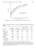
3.4 Example 3.4: Relative Mortality and Identification of
Prognostic Factors, 32
3.5 Example 3.5: Identification of Risk Factors, 40
Bibliographical Remarks, 47
Exercises, 47
vii
4 Nonparametric Methods of Estimating Survival Functions 64
4.1 Product-Limit Estimates of Survivorship Function, 65
4.2 Life-Table Analysis, 77
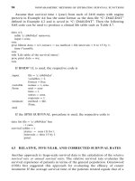
4.3 Relative, Five-Year, and Corrected Survival Rates, 94
4.4 Standardized Rates and Ratios, 97
Bibliographical Remarks, 102
Exercises, 102

5 Nonparametric Methods for Comparing Survival Distributions 106
5.1 Comparison of Two Survival Distributions, 106
5.2 Mantel—Haenszel Test, 121
5.3 Comparison of K (K 92) Samples, 125
Bibliographical Remarks, 131
Exercises, 131
6 Some Well-Known Parametric Survival Distributions
and Their Applications 134
6.1 Exponential Distribution, 134
6.2 Weibull Distribution, 138
6.3 Lognormal Distribution, 143
6.4 Gamma and Generalized Gamma Distributions, 148
6.5 Log-Logistic Distribution, 154
6.6 Other Survival Distributions, 155
Bibliographical Remarks, 160
Exercises, 160
7 Estimation Procedures for Parametric Survival Distributions
without Covariates 162
7.1 General Maximum Likelihood Estimation Procedure, 162
7.2 Exponential Distribution, 166
7.3 Weibull Distribution, 178
7.4 Lognormal Distribution, 180
7.5 Standard and Generalized Gamma Distributions, 188
7.6 Log-Logistic Distribution, 195
7.7 Other Parametric Survival Distributions, 196
Bibliographical Remarks, 196
Exercises, 197
viii 
8 Graphical Methods for Survival Distribution Fitting 198
8.1 Introduction, 198

8.2 Probability Plotting, 200
8.3 Hazard Plotting, 209
8.4 Cox—Snell Residual Method, 215
Bibliographical Remarks, 219
Exercises, 219
9 Tests of Goodness of Fit and Distribution Selection 221
9.1 Goodness-of-Fit Test Statistics Based on Asymptotic
Likelihood Inferences, 222
9.2 Tests for Appropriateness of a Family of Distributions, 225
9.3 Selection of a Distribution Using BIC
or AIC Procedures, 230
9.4 Tests for a Specific Distribution with
Known Parameters, 233
9.5 Hollander and Proschan’s Test for Appropriateness
of a Given Distribution with Known Parameters, 236
Bibliographical Remarks, 238
Exercises, 240
10 Parametric Methods for Comparing Two Survival Distributions 243
10.1 Likelihood Ratio Test for Comparing Two Survival
Distributions, 243
10.2 Comparison of Two Exponential Distributions, 246
10.3 Comparison of Two Weibull Distributions, 251
10.4 Comparison of Two Gamma Distributions, 252
Bibliographical Remarks, 254
Exercises, 254
11 Parametric Methods for Regression Model Fitting and
Identification of Prognostic Factors 256
11.1 Preliminary Examination of Data, 257
11.2 General Structure of Parametric Regression Models
and Their Asymptotic Likelihood Inference, 259

11.3 Exponential Regression Model, 263
11.4 Weibull Regression Model, 269
11.5 Lognormal Regression Model, 274
11.6 Extended Generalized Gamma Regression Model, 277
 ix
11.7 Log-Logistic Regression Model, 280
11.8 Other Parametric Regression Models, 283
11.9 Model Selection Methods, 286
Bibliographical Remarks, 295
Exercises, 295
12 Identification of Prognostic Factors Related to Survival Time:
Cox Proportional Hazards Model 298
12.1 Partial Likelihood Function for Survival Times, 298
12.2 Identification of Significant Covariates, 314
12.3 Estimation of the Survivorship Function with Covariates, 319
12.4 Adequacy Assessment of the Proportional Hazards Model, 326
Bibliographical Remarks, 336
Exercises, 337
13 Identification of Prognostic Factors Related to Survival Time:
Nonproportional Hazards Models 339
13.1 Models with Time-Dependent Covariates, 339
13.2 Stratified Proportional Hazards Models, 348
13.3 Competing Risks Model, 352
13.4 Recurrent Events Models, 356
13.5 Models for Related Observations, 374
Bibliographical Remarks, 376
Exercises, 376
14 Identification of Risk Factors Related to Dichotomous
and Polychotomous Outcomes 377
14.1 Univariate Analysis, 378

14.2 Logistic and Conditional Logistic Regression Models
for Dichotomous Responses, 385
14.3 Models for Polychotomous Outcomes, 413
Bibliographical Remarks, 425
Exercises, 425
Appendix A Newton Raphson Method 428
Appendix B Statistical Tables 433
References 488
Index 511
x 
Preface
Statistical methods for survival data analysis have continued to flourish in the
last two decades. Applications of the methods have been widened from their
historical use in cancer and reliability research to business, criminology,
epidemiology, and social and behavioral sciences. The third edition of Statisti-
cal Methods for Survival Data Analysis is intended to provide a comprehensive
introduction of the most commonly used methods for analyzing survival data.
It begins with basic definitions and interpretations of survival functions. From
there, the reader is guided through methods, parametric and nonparametric,
for estimating and comparing these functions and the search for a theoretical
distribution (or model) to fit the data. Parametric and nonparametric ap-
proaches to the identification of prognostic factors that are related to survival
are then discussed. Finally, regression methods, primarily linear logistic re-
gression models, to identify risk factors for dichotomous and polychotomous
outcomes are introduced.
The third edition continues to be application-oriented, with a minimum
level of mathematics. In a few chapters, some knowledge of calculus and matrix
algebra is needed. The few sections that introduce the general mathematical
structure for the methods can be skipped without loss of continuity. A large
number of practical examples are given to assist the reader in understanding

the methods and applications and in interpreting the results. Readers with only
college algebra should find the book readable and understandable.
There are many excellent books on clinical trials. We therefore have deleted
the two chapters on the subject that were in the second edition. Instead, we
have included discussions of more statistical methods for survival data analysis.
A brief summary of the improvements made for the third edition is given
below.
1. Two additional distributions, the log-logistic distribution and a general-
ized gamma distribution, have been added to the application of paramet-
ric models that can be used in model fitting and prognostic factor
identification (Chapters 6, 7, and 11).
xi
2. In several sections (Sections 7.1, 9.1, 10.1, 11.2, and 12.1), discussions of
the asymptotic likelihood inference of the methods covered in the
chapters are given. These sections are intended to provide a more general
mathematical structure for statisticians.
3. The Cox—Snell residual method has been added to the chapter on
graphical methods for survival distribution fitting (Chapter 8). In addi-
tion, the sections on probability and hazard plotting have been revised
so that no special graphical papers are required to make the plots.
4. More tests of goodness of fit are given, including the BIC and AIC
procedures (Chapters 9 and 11).
5. For Cox’s proportional hazards model (Chapter 12), we have now
included methods to assess its adequency and procedures to estimate the
survivorship function with covariates.
6. The concept of nonproportional hazards models is introduced (Chapter
13), which includes models with time-dependent covariates, stratified
models, competing risks models, recurrent event models, and models for
related observations.
7. The chapter on linear logistic regression (Chapter 14) has been expanded

to cover regression models for polychotomous outcomes. In addition,
methods for a general m : n matching design have been added to the
section on conditional logistic regression for case—control studies.
8. Computer programming codes for software packages BMDP, SAS, and
SPSS are provided for most examples in the text.
We would like to thank the many researchers, teachers, and students who
have used the second edition of the book. The suggestions for improvement
that many of them have provided are invaluable. Special thanks go to Xing
Wang, Linda Hutton, Tracy Mankin, and Imran Ahmed for typing the
manuscript. Steve Quigley of John Wiley convinced us to work on a third
edition. We thank him for his enthusiasm.
Finally, we are most grateful to our families, Sam, Vivian, Benedict, Jennifer,
and Annelisa (E.T.L.), and Alice and Xing (J.W.W.), for the constant joy, love,
and support they have given us.
E T. L
J W W
Oklahoma City, OK
April 18, 2001
xii 
CHAPTER 1
Introduction
1.1 PRELIMINARIES
This book is for biomedical researchers, epidemiologists, consulting statisti-
cians, students taking a first course on survival data analysis, and others
interested in survival time study. It deals with statistical methods for analyzing
survival data derived from laboratory studies of animals, clinical and epi-
demiologic studies of humans, and other appropriate applications.
Survival time can be defined broadly as the time to the occurrence of a given
event. This event can be the development of a disease, response to a treatment,
relapse, or death. Therefore, survival time can be tumor-free time, the time from

the start of treatment to response, length of remission, and time to death.
Survival data can include survival time, response to a given treatment, and
patient characteristics related to response, survival, and the development of a
disease. The study of survival data has focused on predicting the probability of
response, survival, or mean lifetime, comparing the survival distributions of
experimental animals or of human patients and the identification of risk and/or
prognostic factors related to response, survival, and the development of a
disease. In this book, special consideration is given to the study of survival data
in biomedical sciences, although all the methods are suitable for applications
in industrial reliability, social sciences, and business. Examples of survival data
in these fields are the lifetime of electronic devices, components, or systems
(reliability engineering); felons’ time to parole (criminology); duration of first
marriage (sociology); length of newspaper or magazine subscription (market-
ing); and worker’s compensation claims (insurance) and their various influenc-
ing risk or prognostic factors.
1.2 CENSORED DATA
Many researchers consider survival data analysis to be merely the application
of two conventional statistical methods to a special type of problem: parametric
if the distribution of survival times is known to be normal and nonparametric
1
if the distribution is unknown. This assumption would be true if the survival
times of all the subjects were exact and known; however, some survival times
are not. Further, the survival distribution is often skewed, or far from being
normal. Thus there is a need for new statistical techniques. One of the most
important developments is due to a special feature of survival data in the life
sciences that occurs when some subjects in the study have not experienced the
event of interest at the end of the study or time of analysis. For example, some
patients may still be alive or disease-free at the end of the study period. The
exact survival times of these subjects are unknown. These are called censored
observations or censored times and can also occur when people are lost to

follow-up after a period of study. When these are not censored observations,
the set of survival times is complete. There are three types of censoring.
Type I Censoring
Animal studies usually start with a fixed number of animals, to which the
treatment or treatments is given. Because of time and/or cost limitations, the
researcher often cannot wait for the death of all the animals. One option is to
observe for a fixed period of time, say six months, after which the surviving
animals are sacrificed. Survival times recorded for the animals that died during
the study period are the times from the start of the experiment to their death.
These are called exact or uncensored observations. The survival times of the
sacrificed animals are not known exactly but are recorded as at least the length
of the study period. These are called censored observations. Some animals could
be lost or die accidentally. Their survival times, from the start of experiment
to loss or death, are also censored observations. In type I censoring, if there are
no accidental losses, all censored observations equal the length of the study
period.
For example, suppose that six rats have been exposed to carcinogens by
injecting tumor cells into their foot pads. The times to develop a tumor of a
given size are observed. The investigator decides to terminate the experiment
after 30 weeks. Figure 1.1 is a plot of the development times of the tumors.
Rats A, B, and D developed tumors after 10, 15, and 25 weeks, respectively.
Rats C and E did not develop tumors by the end of the study; their tumor-free
times are thus 30-plus weeks. Rat F died accidentally without tumors after 19
weeks of observation. The survival data (tumor-free times) are 10, 15, 30
;
, 25,
30
;
, and 19
;

weeks. (The plus indicates a censored observation.)
Type II Censoring
Another option in animal studies is to wait until a fixed portion of the animals
have died, say 80 of 100, after which the surviving animals are sacrificed. In
this case, type II censoring, if there are no accidental losses, the censored
observations equal the largest uncensored observation. For example, in an
experiment of six rats (Figure 1.2), the investigator may decide to terminate the
study after four of the six rats have developed tumors. The survival or
tumor-free times are then 10, 15, 35
;
, 25, 35, and 19
;
weeks.
2 
Figure 1.1 Example of type I censored data.
Figure 1.2 Example of type II censored data.
Type III Censoring
In most clinical and epidemiologic studies the period of study is fixed and
patients enter the study at different times during that period. Some may die
before the end of the study; their exact survival times are known. Others may
withdraw before the end of the study and are lost to follow-up. Still others may
be alive at the end of the study. For ‘‘lost’’ patients, survival times are at least
from their entrance to the last contact. For patients still alive, survival times
are at least from entry to the end of the study. The latter two kinds of
observations are censored observations. Since the entry times are not simulta-
neous, the censored times are also different. This is type III censoring. For
example, suppose that six patients with acute leukemia enter a clinical study
  3
Figure 1.3 Example of type III censored data.
during a total study period of one year. Suppose also that all six respond to

treatment and achieve remission. The remission times are plotted in Figure 1.3.
Patients A, C, and E achieve remission at the beginning of the second, fourth,
and ninth months, and relapse after four, six, and three months, respectively.
Patient B achieves remission at the beginning of the third month but is lost to
follow-up four months later; the remission duration is thus at least four
months. Patients D and F achieve remission at the beginning of the fifth and
tenth months, respectively, and are still in remission at the end of the study;
their remission times are thus at least eight and three months. The respective
remission times of the six patients are 4, 4
;
,6,8
;
, 3, and 3
;
months.
Type I and type II censored observations are also called singly censored
data, and type III, progressively censored data, by Cohen (1965). Another
commonly used name for type III censoring is random censoring. All of these
types of censoring are right censoring or censoring to the right. There are also
left censoring and interval censoring cases. L eft censoring occurs when it is
known that the event of interest occurred prior to a certain time t, but the exact
time of occurrence is unknown. For example, an epidemiologist wishes to know
the age at diagnosis in a follow-up study of diabetic retinopathy. At the time of
the examination, a 50-year-old participant was found to have already develop-
ed retinopathy, but there is no record of the exact time at which initial evidence
was found. Thus the age at examination (i.e., 50) is a left-censored observation.
It means that the age of diagnosis for this patient is at most 50 years.
Interval censoring occurs when the event of interest is known to have
occurred between times a and b. For example, if medical records indicate that
at age 45, the patient in the example above did not have retinopathy, his age

at diagnosis is between 45 and 50 years.
We will study descriptive and analytic methods for complete, singly cen-
sored, and progressively censored survival data using numerical and graphical
4 
techniques. Analytic methods discussed include parametric and nonparametric.
Parametric approaches are used either when a suitable model or distribution
is fitted to the data or when a distribution can be assumed for the population
from which the sample is drawn. Commonly used survival distributions are the
exponential, Weibull, lognormal, and gamma. If a survival distribution is found
to fit the data properly, the survival pattern can then be described by the
parameters in a compact way. Statistical inference can be based on the
distribution chosen. If the search for an appropriate model or distribution is
too time consuming or not economical or no theoretical distribution adequate-
ly fits the data, nonparametric methods, which are generally easy to apply,
should be considered.
1.3 SCOPE OF THE BOOK
This book is divided into four parts.
Part I (Chapters 1, 2, and 3) defines survival functions and gives examples
of survival data analysis. Survival distribution is most commonly described by
three functions: the survivorship function (also called the cumulative survival
rate or survival function), the probability density function, and the hazard
function (hazard rate or age-specific rate). In Chapter 2 we define these three
functions and their equivalence relationships. Chapter 3 illustrates survival
data analysis with five examples taken from actual research situations. Clinical
and laboratory data are systematically analyzed in progressive steps and the
results are interpreted. Section and chapter numbers are given for quick
reference. The actual calculations are given as examples or left as exercises in
the chapters where the methods are discussed. Four sets of data are provided
in the exercise section for the reader to analyze. These data are referred to in
the various chapters.

In Part II (Chapters 4 and 5) we introduce some of the most widely used
nonparametric methods for estimating and comparing survival distributions.
Chapter 4 deals with the nonparametric methods for estimating the three
survival functions: the Kaplan and Meier product-limit (PL) estimate and the
life-table technique (population life tables and clinical life tables). Also covered
is standardization of rates by direct and indirect methods, including the
standardized mortality ratio. Chapter 5 is devoted to nonparametric tech-
niques for comparing survival distributions. A common practice is to compare
the survival experiences of two or more groups differing in their treatment or
in a given characteristic. Several nonparametric tests are described.
Part III (Chapters 6 to 10) introduces the parametric approach to survival
data analysis. Although nonparametric methods play an important role in
survival studies, parametric techniques cannot be ignored. In Chapter 6 we
introduce and discuss the exponential, Weibull, lognormal, gamma, and
log-logistic survival distributions. Practical applications of these distributions
taken from the literature are included.
    5
An important part of survival data analysis is model or distribution fitting.
Once an appropriate statistical model for survival time has been constructed
and its parameters estimated, its information can help predict survival, develop
optimal treatment regimens, plan future clinical or laboratory studies, and so
on. The graphical technique is a simple informal way to select a statistical
model and estimate its parameters. When a statistical distribution is found to
fit the data well, the parameters can be estimated by analytical methods. In
Chapter 7 we discuss analytical estimation procedures for survival distribu-
tions. Most of the estimation procedures are based on the maximum likelihood
method. Mathematical derivations are omitted; only formulas for the estimates
and examples are given. In Chapter 8 we introduce three kinds of graphical
methods: probability plotting, hazard plotting, and the Cox—Snell residual
method for survival distribution fitting. In Chapter 9 we discuss several tests

of goodness of fit and distribution selection. In Chapter 10 we describe several
parametric methods for comparing survival distributions.
A topic that has received increasing attention is the identification of
prognostic factors related to survival time. For example, who is likely to
survive longest after mastectomy, and what are the most important factors that
influence that survival? Another subject important to both biomedical re-
searchers and epidemiologists is identification of the risk factors related to the
development of a given disease and the response to a given treatment. What
are the factors most closely related to the development of a given disease? Who
is more likely to develop lung cancer, diabetes, or coronary disease? In many
diseases, such as cancer, patients who respond to treatment have a better
prognosis than patients who do not. The question, then, relates to what the
factors are that influence response. Who is more likely to respond to treatment
and thus perhaps survive longer?
Part IV (Chapters 11 to 14) deals with prognostic/risk factors and survival
times. In Chapter 11 we introduce parametric methods for identifying impor-
tant prognostic factors. Chapters 12 and 13 cover, respectively, the Cox
proportional hazards model and several nonproportional hazards models for
the identification of prognostic factors. In the final chapter, Chapter 14, we
introduce the linear logistic regression model for binary outcome variables and
its extension to handle polychotomous outcomes.
In Appendix A we describe a numerical procedure for solving nonlinear
equations, the Newton—Raphson method. This method is suggested in Chap-
ters 7, 11, 12, and 13. Appendix B comprises a number of statistical tables.
Most nonparametric techniques discussed here are easy to understand and
simple to apply. Parametric methods require an understanding of survival
distributions. Unfortunately, most of survival distributions are not simple.
Readers without calculus may find it difficult to apply them on their own.
However, if the main purpose is not model fitting, most parametric techniques
can be substituted for by their nonparametric competitors. In fact, a large

percentage of survival studies in clinical or epidemiological journals are
analyzed by nonparametric methods. Researchers not interested in survival
6 
model fitting should read the chapters and sections on nonparametric methods.
Computer programs for survival data analysis are available in several commer-
cially available software packages: for example, BMDP, SAS, and SPSS. These
computer programs are referred to in various chapters when applicable.
Computer programming codes are given for many of the examples.
Bibliographical Remarks
Cross and Clark (1975) was the first book to discuss parametric models and
nonparametric and graphical techniques for both complete and censored
survival data. Since then, several other books have been published in addition
to the first edition of this book (Lee, 1980, 1992). Elandt-Johnson and Johnson
(1980) discuss extensively the construction of life tables, model fitting, compet-
ing risk, and mathematical models of biological processes of disease pro-
gression and aging. Kalbfleisch and Prentice (1980) focus on regression
problems with survival data, particularly Cox’s proportional hazards model.
Miller (1981) covers a number of parametric and nonparametric methods for
survival analysis. Cox and Oakes (1984) also cover the topic concisely with an
emphasis on the examination of explanatory variables.
Nelson (1982) provides a good discussion of parametric, nonparametric, and
graphical methods. The book is more suited for industrial reliability engineers
than for biomedical researchers, as are Hahn and Shapiro (1967) and Mann et
al. (1974). In addition, Lawless (1982) gives a broad coverage of the area with
applications in engineering and biomedical sciences.
More recent publications include Marubini and Valsecchi (1994), Klein-
baum (1995), Klein and Moeschberger (1997), and Hosmer and Lemeshow
(1999). Most of these books take a more rigorous mathematical approach and
require knowledge of mathematical statistics.
    7

CHAPTER 2
Functions of Survival Time
Survival time data measure the time to a certain event, such as failure, death,
response, relapse, the development of a given disease, parole, or divorce. These
times are subject to random variations, and like any random variables, form a
distribution. The distribution of survival times is usually described or charac-
terized by three functions: (1) the survivorship function, (2) the probability
density function, and (3) the hazard function. These three functions are
mathematically equivalent — if one of them is given, the other two can be
derived.
In practice, the three functions can be used to illustrate different aspects of
the data. A basic problem in survival data analysis is to estimate from the
sampled data one or more of these three functions and to draw inferences
about the survival pattern in the population. In Section 2.1 we define the three
functions and in Section 2.2, discuss the equivalence relationship among the
three functions.
2.1 DEFINITIONS
Let T denote the survival time. The distribution of T can be characterized by
three equivalent functions.
Survivorship Function (or Survival Function)
This function, denoted by S(t), is defined as the probability that an individual
survives longer than t:
S(t) : P (an individual survives longer than t)
: P(T 9t) (2.1.1)
From the definition of the cumulative distribution function F(t)ofT,
S(t) : 1-P (an individual fails before t)
: 1 9 F(t)(2.1.2)
8
Figure 2.1 Two examples of survival curves.
Here S(t) is a nonincreasing function of time t with the properties

S(t) :

1 for t : 0
0 for t : -
That is, the probability of surviving at least at the time zero is 1 and that of
surviving an infinite time is zero.
The function S(t) is also known as the cumulative survival rate. To depict the
course of survival, Berkson (1942) recommended a graphic presentation of S(t).
The graph of S(t) is called the survival curve. A steep survival curve, such as
the one shown in Figure 2.1a, represents low survival rate or short survival
time. A gradual or flat survival curve such as in Figure 2.1b represents high
survival rate or longer survival.
The survivorship function or the survival curve is used to find the 50th
percentile (the median) and other percentiles (e.g., 25th and 75th) of survival
time and to compare survival distributions of two or more groups. The median
survival times in Figure 2.1a and b are approximately 5 and 36 units of time,
respectively. The mean is generally used to describe the central tendency of a
distribution, but in survival distributions the median is often better because a
small number of individuals with exceptionally long or short lifetimes will
cause the mean survival time to be disproportionately large or small.
In practice, if there are no censored observations, the survivorship function
is estimated as the proportion of patients surviving longer than t :
S (t) :
number of patients surviving longer than t
total number of patients
(2.1.3)
where the circumflex denotes an estimate of the function. When censored
observations are present, the numerator of (2.1.3) cannot always be determined.
For example, consider the following set of survival data: 4, 6, 6
;

,10
;
, 15, 20.
 9
Figure 2.2 Two examples of density curves.
Using (2.1.3), we can compute S (5) : 5/6 : 0.833. However, we cannot obtain
S (11) since the exact number of patients surviving longer than 11 is unknown.
Either the third or the fourth patient (6
;
and 10
;
) could survive longer than
or less than 11. Thus, when censored observations are present, (2.1.3) is no
longer appropriate for estimating S(t). Nonparametric methods of estimating
S(t) for censored data are discussed in Chapter 4.
Probability Density Function (or Density Function)
Like any other continuous random variable, the survival time T has a
probability density function defined as the limit of the probability that an
individual fails in the short interval t to t ; t per unit width t, or simply the
probability of failure in a small interval per unit time. It can be expressed as
f (t) :
lim
R
P[an individual dying in the interval (t, t ; t)]
t
(2.1.4)
The graph of f (t) is called the density curve. Figure 2.2a and b give two
examples of the density curve. The density function has the following two
properties:
1. f (t) is a nonnegative function:

f (t) . 0 for all t .0
: 0 for t :0
2. The area between the density curve and the t axis is equal to 1.
In practice, if there are no censored observations, the probability density
function f (t) is estimated as the proportion of patients dying in an interval per
10    
unit width:
f (t) :
number of patients dying in the interval beginning at time t
(total number of patients);(interval width)
(2.1.5)
Similar to the estimation of S(t), when censored observations are present,
(2.1.5) is not applicable. We discuss an appropriate method in Chapter 4.
The proportion of individuals that fail in any time interval and the peaks of
high frequency of failure can be found from the density function. The density
curve in Figure 2.2a gives a pattern of high failure rate at the beginning of the
study and decreasing failure rate as time increases. In Figure 2.2b, the peak of
high failure frequency occurs at approximately 1.7 units of time. The propor-
tion of individuals that fail between 1 and 2 units of time is equal to the shaded
area between the density curve and the axis. The density function is also known
as the unconditional failure rate.
Hazard Function
The hazard function h(t) of survival time T gives the conditional failure rate.
This is defined as the probability of failure during a very small time interval,
assuming that the individual has survived to the beginning of the interval, or
as the limit of the probability that an individual fails in a very short interval,
t ; t, given that the individual has survived to time t:
h(t) :
lim
R

P

an individual fails in the time interval (t, t ; t)
given the individual has survived to t

t
(2.1.6)
The hazard function can also be defined in terms of the cumulative
distribution function F(t) and the probability density function f (t):
h(t) :
f (t)
1 9 F(t)
(2.1.7)
The hazard function is also known as the instantaneous failure rate, force of
mortality, conditional mortality rate, and age-specific failure rate. If t in (2.1.6)
is age, it is a measure of the proneness to failure as a function of the age of the
individual in the sense that the quantity th(t) is the expected proportion of
age t individuals who will fail in the short time interval t ;t. The hazard
function thus gives the risk of failure per unit time during the aging process. It
plays an important role in survival data analysis.
In practice, when there are no censored observations the hazard function is
estimated as the proportion of patients dying in an interval per unit time, given
 11