The Options Course High Profit & Low Stress Trading Methods Second Edition phần 6 pptx

$1,000, which is also the maximum reward. The maximum risk is calcu-
lated by subtracting the net credit ($200) from the difference in strikes (95
– 90 = 5). This creates a maximum risk of $300: (5 – 2) × 100 = $300. If IBM
were to close anywhere between $85 and $90 on expiration, the maximum
profit of $200 per contract, or $1,000 (for five contracts), could be kept.
The breakeven points were at $83 and $92 and are found by taking the net
credit of $2 and subtracting it from the lower sold strike for the lower
breakeven. The upper breakeven is found by adding the $2 credit to the
higher sold option strike.
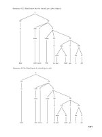
Notice how the risk graph (see Figure 10.6) shows limited reward
and limited risk. The risk graph also points out that the maximum profit
is impossible to achieve until expiration. This strategy rarely sees a
280 THE OPTIONS COURSE
Profit
–1500 –1000 0 1000
70 80 90 100
Today: 36 days left Close= 89.28
24 days left
12 days left
Expiry: 0 days left
FIGURE 10.6 Risk Graph of Long Iron Butterfly on IBM (Source: Optionetics
Platinum © 2004)
ccc_fontanills_ch10_265-310.qxd 12/17/04 4:16 PM Page 280
trader get out with a profit at the beginning of the trade. This is because
an iron butterfly benefits from time erosion. We aren’t going to see as
high a reward-to-risk ratio trading an iron butterfly, but our maximum
profit is more likely to be achieved because of the wider maximum
profit range.
IBM shares did indeed trade sideways through November expiration,
closing at $88.63 on November 21. This left this trade with the maximum
profit of $1,000. If the stock had closed above 95 or below 80, the maxi-

mum loss would have occurred.
CALENDAR SPREAD
A calendar spread is a trade that can be used when the trader expects a
gradual or sideways move in the stock. Sometimes called the horizontal
spread, it uses two options with the same strike prices and different expi-
ration dates. It can be created with puts or calls. Generally, with the cal-
endar spread, the option strategist is buying a longer-term option and
selling a shorter-term option. Unlike the vertical spreads like bull call
spreads, bear put spreads, and other trades that are directional in nature
(i.e., they require the shares to move higher or lower), calendar spreads
Trading Techniques for Range-Bound Markets 281
Long Iron Butterfly Case Study
Strategy: With the security trading at $89.28 a share on October 16,
2003, Long 5 November IBM 80 Puts @ 0.35, Short 5 November IBM 85
Puts @ 0.95, Short 5 November IBM 90 Calls @ 2, and Long 5 November
IBM 95 Calls @ 0.60.
Market Opportunity: Expect stock to stay in narrow range through
November expiration.
Maximum Profit: Limited to the net credit. In this case, $1,000: {5 × [(.95
+ 2.00) – (.35 + .60)]} × 100.
Maximum Risk: Limited to difference in strikes minus the net credit. In
this case, $1,500: 5 × [(5 – 2) × 100].
Lower Breakeven: Lower short strike minus the net credit. In this case,
83: (85 – 2).
Upper Breakeven: Higher short strike plus the net credit. In this case,
92: (90 + 2).
Margin: Minimal—just enough to cover the broker’s risk.
ccc_fontanills_ch10_265-310.qxd 12/17/04 4:16 PM Page 281
can be created when the strategist is neutral on the shares. Basically, in a
neutral calendar spread, the trader wants the short-term option to decay

at a faster rate than the long-term option. However, strategists can also
create both bullish and bearish calendar spreads depending on their out-
look for the shares.
Calendar Spread Mechanics
Let’s consider an example of the calendar spread using XYZ at $50 a
share in March. In this case, we expect the shares to stay at roughly the
same levels or move modestly higher. Consequently, we decide to pur-
chase a LEAPS long-term option and offset some of the cost of that op-
tion with the sale of a shorter-term option. In this case, we buy the XYZ
60 LEAPS at $4 and sell an XYZ 60 call with two months of life remaining
at $1. The cost of the trade is $300 [(4 – 1) × 100 = $300], which is also
the maximum risk associated with this trade. The maximum profit is un-
limited once the short-term option expires. At that point, the trade is
simply a long call.
Prior to the expiration of the short call, the maximum profit and
breakeven will depend on a number of factors including volatility, the
stock price, and the amount of time decay suffered by the long call. Basi-
cally, it is impossible to determine how much value the long call will
gain or lose during the life of the short option. Options trading software,
such as the Optionetics.com Platinum site, can help give a better sense
of the risk, rewards, and breakevens associated with any particular cal-
endar spread. For now, suffice it to say that the risk is limited to the net
debit. In addition, time decay is not linear. That is, an option with 30
days until expiration will lose value more rapidly than an option with six
months until expiration. Calendar spreads attempt to take advantage of
the fact that short-term options suffer time decay at a faster rate than
long-term options.
Computing breakeven prices for complex trades requires the use of
computer software. To understand why, let’s consider a bullish calendar
spread. In this case, we are buying a longer-term call and selling a shorter-

term call with the same strike price. The trade is placed for a debit and
closed for a credit. Ideally, the short-term call will expire worthless, but
the longer-term call will retain most or all of its value. In that case, we can
sell another call or close the trade at a profit. The breakeven price for the
calendar spread will depend on the value of the long call when the short
option expires. The value of the long call will, in turn, depend on several
factors. Say, for example, the stock price falls and the short call expires
worthless. The long-term option might still have value, but we don’t know
282 THE OPTIONS COURSE
ccc_fontanills_ch10_265-310.qxd 12/17/04 4:16 PM Page 282
exactly how much value because of changes in implied volatility and time
decay. To break even, the value of the long call when it is sold must be
equal to the debit paid for the calendar spread. If the call is worth more,
and the spread is closed when the short option expires, the trade yields a
profit. However, it is impossible to calculate the exact value of the long
call, and therefore, the breakeven when the short call expires. It is possi-
ble to get an idea or rough guess, but it is better to use computer soft-
ware to plot the risk graph and see where the potential breakeven points
might be.
Exiting the Position
The exit strategy for the calendar spread is extremely important in de-
termining the trade’s success. Specifically, if the shares remain range-
bound and the short call expires worthless, the strategist must make a
decision: (1) to exit the position, (2) to sell another call, or (3) to roll up
to another strike price. Generally, if the shares are stable as anticipated,
the best approach is to sell another shorter-term option. In our example,
the long call has 18 months until expiration and was purchased for $4. A
call with three months can be sold for $1. If, over the course of 18
months, calls with three months until expiration can be sold for $1 five
times, the credit received from selling those calls totals $5. The cost of

the long option is only $4. Therefore, the trade yields a $1 profit on a $4
investment, or 25 percent over the course of 15 months. Furthermore,
after 15 months, the long call, which has been fully paid for, will still
have three months of life remaining and can offer upside rewards in case
XYZ marches higher.
Sometimes, however, it is not possible to sell another call. Instead,
the share price jumps too high and the risk profile associated with sell-
ing another call is not attractive. In that case, the strategist might sim-
ply want to close the position by selling the long call. Or another
calendar spread can be established on the same shares by rolling up to
a higher strike price. In that case, the strategist closes the long call,
buys back another long call with a higher strike price, and then sells a
shorter-term call with the same strike price. If the shares move against
the strategist during the life of the short call, the best approach is prob-
ably to exit the entire position once the short call has little time value
remaining. If the shares jump higher and the long call has significant
time value, it is better to close the position rather than face assignment
or buy back the short option. If assigned and forced to exercise the long
option to cover the assignment, the strategist will lose the time value
still left in the long contract.
Trading Techniques for Range-Bound Markets 283
ccc_fontanills_ch10_265-310.qxd 12/17/04 4:16 PM Page 283
Calendar Spread Case Study
Shares of Johnson & Johnson (JNJ) are trading for $51.75 during the
month of February and the strategist expects the shares to make a move
higher. A bullish calendar spread is created by purchasing a JNJ January
2005 60 call for $4 and selling an April 2003 60 call for $1. The trade costs
$300: (4 – 1) × 100 = $300. Therefore, the initial debit in the account is
equal to $300. The debit is also the maximum risk associated with this
trade. As the price of the shares rises, the trade makes money.

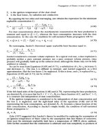
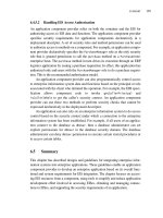
As we can see from the risk graph in Figure 10.7, the maximum profit
occurs when the shares reach $60 at April expiration and is equal to
roughly $570. At that point, the short call expires worthless, but the long
284
THE OPTIONS COURSE
Calendar Spread
Strategy: Sell a short-term option and buy a long-term option using ATM
options with as small a net debit as possible (all calls or all puts). Calls can
be used for a more bullish bias and puts can be used for a more bearish bias.
Market Opportunity: Look for a range-bound market that is expected to
stay between the breakeven points for an extended period of time.
Maximum Risk: Limited to the net debit paid. (Long premium – short pre-
mium) × 100.
Maximum Profit: Limited. Use software for accurate calculation.
Breakeven: Use software for accurate calculation.
Margin: Amount subject to broker’s discretion.
Calendar Spread Case Study
Market Opportunity: JNJ is expected to trade moderately higher. With
shares near $51.75 in February, the strategist sells an April 60 call for $1
and buys a January 2005 60 call for $4.
Maximum Risk: Limited to the net debit. In this case, $300: (4 – 1) × 100.
Maximum Profit: Limited due to the fact that the short call is subject to
assignment risk if shares rise above $60.
Upside Breakeven: Use options software to calculate. In this case,
roughly $47.
Downside Breakeven: Use options software to calculate. In this case,
same as upside breakeven.
Margin: Theoretically, zero. The short call is covered by the long call.
Check with your broker.
ccc_fontanills_ch10_265-310.qxd 12/17/04 4:16 PM Page 284

call has appreciated in value and can be sold at a profit. If the strategist
elects to hold the long call instead, another calendar spread can be estab-
lished by selling a shorter-term call. At that point, the risk curve will prob-
ably look different. The downside breakeven is 46.80. Below that, the
trade begins to lose money. An options trading software program like Plat-
inum can be used to compute the maximum gain and the breakevens.
In this case study, the stock did indeed move in the desired direction.
By April expiration, shares of JNJ fetched $55.35 a share. At that point, the
short call would expire worthless and the strategist would keep the entire
premium received for selling the April 60 call. Meanwhile, the January 60
call has not only retained all of its value, but it is currently offered for
$5.10. Therefore, the strategist’s earnings are $210 of profit per spread ($1
received for the premium and $1.10 profit for the appreciation in the Janu-
ary 60 call), for a five-month 70 percent gain. On the other hand, the strate-
gist could also hold the long call and sell another short-term call with the
same or higher strike price. If the strategist chooses to sell a call with a
higher strike price, the position becomes a diagonal spread, which is also
our next subject of discussion.
VOLATILITY SKEWS REVISITED
As we have seen, calendar spreads are trades that involve the purchase
and sale of options on the same shares, with the same strike price, but dif-
ferent expiration dates. One thing to look for when searching for calendar
Trading Techniques for Range-Bound Markets 285
Profit
–200 –100 0 100 200 300 400 500
40 50 60
Today: 63 days left Close= 51.75
42 days left
21 days left
Expiration

Stock Price
50 60
51.31 52.50 51.20 51.75 +0.44
11/13 12/05 12/27 01/21
Currently: 02-14-03
FIGURE 10.7 JNJ Calendar Spread (Source: Optionetics Platinum © 2004)
ccc_fontanills_ch10_265-310.qxd 12/17/04 4:16 PM Page 285
spreads is a volatility skew. A volatility skew is created when one or more
options have a seeable difference in implied volatility (IV). Implied
volatility, as mentioned in Chapter 9, is a factor that contributes to an op-
tion’s price. All else being equal, an option with high IV is more expensive
than an option with low IV. In addition, two options on the same underly-
ing asset can sometimes have dramatically different levels of volatility.
When this happens, it is known as volatility skew. Looking at various
quotes of options and looking at each option’s IV will reveal potential
volatility skews.
As previously mentioned, there are two types of volatility skews pre-
sent in today’s markets: volatility price skews and volatility time skews.
Volatility price skews exist when two options with the same expiration
date have very different levels of implied volatility. For example, if XYZ is
trading at $50, the XYZ March 55 call has an implied volatility of 80 per-
cent and the XYZ March 60 call has implied volatility of only 40 percent.
Sometimes this happens when there is strong demand for short-term at-
the-money or near-the-money call (due to takeover rumors, an earnings
report, management shake-up, etc.). In that case, the 55 calls have become
much more expensive (higher IV) than the 60 calls.
Calendar spreads can be used to take advantage of the other type of
volatility skew: time skews. This type of skew exists when two options on
the same underlying asset with the same strike prices have different levels
of implied volatility. For example, in January, the XYZ April 60 call has im-

plied volatility of 80 percent and the XYZ December 60 call has implied
volatility of only 40 percent. In that case, the short-term option is more ex-
pensive relative to the long-term call and the calendar spread becomes
more appealing (although the premium will still be greater for the long
call because there will be less time value in the short-term option). The
idea is for the strategist to get more premiums for selling the option with
the higher IV than he or she is paying for the option with the low IV.
DIAGONAL SPREAD
There are a significant number of different ways to structure diagonal
spreads. Diagonal spreads include two options with different expiration
dates and different strike prices. For example, buying a longer-term call
option and selling a shorter-term call option with a higher strike price can
be a way of betting on a rise in the price of the shares. The idea would be
for the shares to rise and cause the long-term option to increase in value.
The short-term call option, which is sold to offset the cost of the long-term
option, will also increase in value. But if the shares stay below the short
286
THE OPTIONS COURSE
ccc_fontanills_ch10_265-310.qxd 12/17/04 4:16 PM Page 286
strike price, the short option expires worthless. In this type of trade, the
longer-term option should have some intrinsic or real value, but the option
sold should have only about 30 days or so to expiration and consist of
nothing but time value. This strategy profits if the shares make a gradual
rise. Similar diagonal spreads can be structured with puts and generate
profits if the shares fall.
Diagonal Spread Example
Diagonal spreads are a common way of taking advantage of volatility
skews. Let’s consider an example to see how. The rumor mill is churning
and there is talk that XYZ is going to be the subject of a hostile takeover.
With shares trading at $50 a share, the rumor is that XYZ will be purchased

for $60 a share. At this point, you have done a lot of research on XYZ and
you believe that the rumor is bogus. Furthermore, you notice that the talk
has created a time volatility skew between the short-term and the long-
term options. In this case, the March 55 call has seen a jump in implied
volatility to 100 percent and trades for $1.50. Meanwhile, the December
contract has seen no change in IV and the December 50 call currently
trades for $6.50.
To take advantage of this skew, the strategist sets up a diagonal
spread by purchasing the December 50 call and selling the March 55 call.
The idea is for the short call to lose value due to time decay and a drop in
implied volatility. Meanwhile, the long-term option will retain most of its
value. The cost of the trade is $5 a contract or $500: (6.50 – 1.50) × 100.
This is the maximum risk associated with the trade.
There are no hard-and-fast rules for computing breakevens and maxi-
mum profits for diagonal spreads. In our example, the ideal scenario would
be for the short option to lose value much faster than the long option due to
both falling IV and time decay. However, the term diagonal spread refers to
any trade that combines different strike prices and different expiration
dates. Therefore, the potential combinations are vast. However, it is possible
to compute the breakevens, risks, and rewards for any trade using options
trading software like the one available at Optionetics.com Platinum site.
Exiting the Position
The same principles that were discussed with respect to calendar spreads
apply to diagonal spreads. If the shares move dramatically higher, the short
option has a greater chance of assignment when it moves in-the-money and
time decay diminishes to a quarter of a point or less. If the long call has sig-
nificant time value, it is better to close the position than face assignment. If
assigned and forced to exercise the long option, the strategist will lose the
Trading Techniques for Range-Bound Markets 287
ccc_fontanills_ch10_265-310.qxd 12/17/04 4:16 PM Page 287

time value still left in the long contract. If the short option expires as antic-
ipated, the strategist can close the position, roll up to a higher strike price,
or simply hold on to the long call.
In the previous example, a diagonal spread was designed to take ad-
vantage of a volatility skew. Once the skew has disappeared and the ob-
jective is achieved the strategist can exit the position by selling the long
call and buying back the short call. However, it generally takes a relatively
large volatility skew in order to profit from changes in implied volatility
alone. Therefore, strategists generally use time decay to their advantage
as well, which, as we saw earlier, impacts shorter-term options to a
greater degree than longer-term options.
In the example, the idea was to take in the expensive (high IV) premium
of the short option and benefit from time decay. As a result, once the short
option expires, there is no reason to keep the long option. Thus, selling an
identical call can close the position. If the shares fall sharply, the trade will
lose value and the strategist wants to begin thinking about mitigating losses.
A sharp move higher could result in assignment on the short call as expira-
tion approaches. Again, it is better to close the position than face assign-
ment because the long option will still have considerable time value, which
would be lost if the long call is exercised to cover the short call.
Breakeven Conundrums
While the risk to the diagonal spread is easy to compute because it is lim-
ited to the net debit paid, and the reward is known in advance because it
is unlimited after the short-term option expires, the breakeven point is a
bit more difficult to calculate. Often, traders first look at the breakeven
price when the short-term option expires. However, at that point in time,
the longer-term option will probably still have value. In addition, the value
of that long option will be difficult to predict ahead of time due to changes
in implied volatility and the impact of time decay.
For example, assume we set up a diagonal spread on XYZ when it is

trading for $53 a share. We buy a long-term call option with a strike price
of 60 for $3 and sell a shorter-term call with a strike price of 55 for $1. The
net debit is $200. Now, let’s assume that at the first expiration the stock is
trading for $54.75 and the short-term option expires worthless. How much
is the longer-term option worth, and what is the breakeven? It is difficult
to predict what the longer-term option will be worth because of the im-
pact of time decay and changes in implied volatility. So, it is impossible to
know the breakeven when the short-term option expires because it will
also depend on the future value of the longer-term option. If the longer-
term option has appreciated enough to cover the cost of the debit when
the short-term option expires, the trade breaks even.
288
THE OPTIONS COURSE
ccc_fontanills_ch10_265-310.qxd 12/17/04 4:16 PM Page 288
After the short-term option expires, the breakeven shifts to the expi-
ration of the longer-term option. In this case, the breakeven price be-
comes the debit plus the strike price, or $62 a share. However, the
breakeven will change again if we take follow-up action like selling an-
other short-term call option.
In sum, it is difficult to know exactly what the breakeven stock price
will be for the diagonal or calendar spread because we are dealing with
options with different expiration dates. In these situations, the best ap-
proach is to use options-trading software to get a general idea. However,
even software is not perfect because it can’t predict future changes in an
option’s future implied volatility. The best we can do is to calculate an ap-
proximate breakeven and then plan our exit strategies accordingly.
Diagonal Spread Case Study
For the diagonal spread case study, let’s consider Johnson & Johnson
(JNJ) trading for $51.75 a share in early February 2003. The strategist sets
up a diagonal spread by purchasing a January 2005 50 call for $6.50 and

selling the March 2003 55 call for $1.50. Again, there is time volatility skew
when purchasing these contracts and the long call has lower IV compared
to the short call. This type of time volatility skew is a favorable character-
istic when setting up this type of diagonal spread.
Trading Techniques for Range-Bound Markets 289
Diagonal Spread
Strategy: Sell a short-term option and buy a long-term option with differ-
ent strikes and as small a net debit as possible (use all calls or all puts).
•A bullish diagonal spread employs a long call with a distant expira-
tion and a lower strike price, along with a short call with a closer expi-
ration date and higher strike price.
•A bearish diagonal spread combines a long put with a distant expi-
ration date and a higher strike price along with a short put with a closer
expiration date and lower strike price.
Market Opportunity: Look for a range-bound market exhibiting a time
volatility skew that is expected to stay between the breakeven points for
an extended period of time.
Maximum Risk: Limited to the net debit paid. (Long premium – short pre-
mium) × 100.
Maximum Profit/Upside Breakeven/Downside Breakeven: Use
options software for accurate calculation, such as the Platinum site at
Optionetics.com.
ccc_fontanills_ch10_265-310.qxd 12/17/04 4:16 PM Page 289
The risk, profit, and breakevens for this trade are relatively straight-
forward. The cost of the trade is $500 and is equal to the premium of the
long call minus the short call times 100: [(6.50 – 1.50) × 100]. The debit is
also the maximum risk associated with this trade. Profits arise if the
shares move higher. The maximum profit during the life of the short call
equals $374.45. After the short call expires, the position is no longer a di-
agonal spread. It is simply a long call. At that point, the strategist can sell,

exercise, or hold the long call.
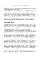
The risk curve of the diagonal spread is plotted in Figure 10.8. It is simi-
lar to the calendar spread. In both cases, the strategist wants the share price
to move higher, but not rise above the strike price of the short call. A move
lower will result in losses. If the stock rises and equals $55 a share at the
March expiration, the short call will expire worthless. The strategist will
keep the premium received from selling the short call and will have a profit
from an increase in the value of the call. At that point, he or she can sell, ex-
ercise, or hold the long call. If the trader elects to hold the long call, another
diagonal spread can be established by selling another shorter-term call.
So, what happened with our JNJ calendar spread? Shortly after the
trade was initiated, shares rallied sharply and, in the week before expira-
tion, the stock was well above the March 55 strike price. At that point, we
would be forced into follow-up action because assignment was all but as-
sured. For example, the week just before expiration, the stock was mak-
ing its move above $55 a share. Seeing this, the strategist would probably
290
THE OPTIONS COURSE
Profit
–400 –300 –200 –100 0 100 200 300
40 50 60
Today: 35 days left Close= 51.75
23 days left
11 days left
Expiration
Stock Price
50 60
51.31 52.50 51.20 51.75 +0.44
11/13 12/05 12/27 01/21
Currently: 02–14–03

FIGURE 10.8 JNJ Diagonal Spread (Source: Optionetics Platinum © 2004)
ccc_fontanills_ch10_265-310.qxd 12/17/04 4:16 PM Page 290
want to buy the short-term call to close because assignment would force
him or her either to buy the stock in the market for more than $55 a share
and sell it at the strike price or cover with the long call, which still has a
significant amount of time value.
So, facing the risk of assignment, the position is closed when the
stock moves toward the strike price of the short call. The Friday before
expiration, the January 2004 50 call was quoted for $8.50 bid. Therefore,
the strategist would book a $2 profit on that side of the trade. At the same
time, he or she would want to buy to close the short March 55 call, which
was offered for $1. That side of the trade would yield a 50-cent profit.
Therefore, taken together, the strategist makes $250 on a $500 investment.
Time decay has indeed worked in this trade’s favor.
The reason I like trading diagonal spreads is that they lend them-
selves to numerous position adjustments during the trade process. For
example, say we initiate a diagonal calendar spread on stock XYZ by pur-
chasing a longer-term ITM call option and writing a shorter-term slightly
OTM call option. This position can be put on at a lower cost than the tra-
ditional covered call and with a subsequent lower risk. It also has a
higher-percentage return than a covered call but still profits from time de-
cay. However, the real advantage of the position in my view is its inherent
flexibility. Consider just some of the adjustments afforded the options
trader with the diagonal spread position:
• XYZ is below the strike price that we initially sold: Let it expire
worthless and realize the short-term call premium as a profit. We can
then exit the long position, or sell another short-term call for the next
month out.
• XYZ is near or above the short strike price by the expiration
date: Buy the short option back and sell back the long position to

close the trade, or sell the next month calls of the same strike or even
a higher strike if the underlying stock has an upward directional bias.
• XYZ is deep in-the-money: Exit the entire position and rebracket
the diagonal spread at the new trading range.
In addition, we can convert from a diagonal spread to a horizontal if
more than 60 days are still left until expiration. If we are going into the fi-
nal 30 days of the long position we can transform this position into a verti-
cal spread. Even though our XYZ example was created using calls, the
trader can also construct this position using put options.
These are just a handful of adjustments afforded the options trader
when managing a diagonal spread. I encourage you to test and paper trade
these types of positions. The adjustment possibilities are virtually endless
and for my money that makes for a terrific options strategy.
Trading Techniques for Range-Bound Markets 291
ccc_fontanills_ch10_265-310.qxd 12/17/04 4:16 PM Page 291
COLLAR SPREAD
Collar spreads are usually one of the first combination option trades a per-
son is exposed to after getting a grasp of what basic puts and calls are all
about. They are usually presented as appreciating collars or protective
collars. However, not much mention is given to the inherent flexibility of
this position and how, as a trader, if you want to put just a little bit more
effort into the trade, you can increase your returns.
There are two types of collar trades: the protective collar and the ap-
preciating collar. The protective collar is chosen when a person already
owns the stock and has a bearish outlook but still wants to hold the stock.
In this case, the trader would purchase an at-the-money put and at the
same time sell an at-the-money call to finance that put. This essentially
locks in the current price and protects the trade from losses until such
time when the bearish scenario changes.
The other type of collar is an appreciating collar. This is the one

where you can make money and indeed trade dynamically if you desire.
The appreciating collar involves buying stock and for every 100 shares of
stock purchased buying an at-the-money put and selling an out-of-the-
money call to finance the put. The key to this strategy is selecting a stock
that has been in the news, whose volatility is high, and for which a type
skew exists (a type skew is when a volatility skew exists between the put
292
THE OPTIONS COURSE
Diagonal Spread Case Study
Strategy: With JNJ trading for $51.75 in February, set up a bullish diago-
nal spread by selling a March 55 call at $1.50 and buying a January 50 call
at $6.50.
Market Opportunity: Anticipate a short-term move higher in a trending
stock. Look for time volatility skew to increase odds of success.
Maximum Risk: Limited to the net debit. In this case, the risk is losing
the premium paid for the long call ($650) minus the premium received for
the short put ($150) for a maximum risk of $500.
Maximum Profit: During the life of the short option, the profit is limited
due to the possibility of assignment. In this case, above $55 a share, the
strategist will be forced to engage in follow-up action.
Upside Breakeven: No set formula. Will vary based on IV assumptions.
Downside Breakeven: No set formula. Will vary based on IV assumptions.
Margin: Amount subject to broker’s discretion.
ccc_fontanills_ch10_265-310.qxd 12/17/04 4:16 PM Page 292
purchased and the call sold). By doing so you will find that your risk will
be reduced to virtually nothing.
Now what if the stock you have chosen gets on a nice steady run and
is at or goes above your appreciating collar strike price? If it is at the
strike price, you can continue to hold and eventually let the calls and
puts expire worthless, and then sell the stock to take your profits. If it is

above the strike price, the calls you sold will carry away the stock and
the put expires worthless; you garner the maximum profit potential of
this position.
To establish a collar, many strategists buy (or already own) the actual
shares, buy an at-the-money LEAPS put, and sell an out-of-the-money
LEAPS call. Doing so combines the covered call with a protective put. In
theory, the call and put that are equidistant from the share price should
carry the same premium. So, if you own a stock at $50 a share and want to
protect the downside risk, you could buy a put. However, the put will cost
money and the premium would be deducted from your account. Another
option is to buy a 45 put and sell a 55 call. The sale of the call will reduce
the cost of the purchase of the put.
Collar Mechanics
Let’s consider an example of a collar using XYZ. During the month of
February, XYZ is trading for $50 a share and an investor has been hold-
ing the shares for some time. She doesn’t expect much movement in the
stock, but believes that there is a 10 percent chance that the price will
decline during the next four months and wants to hedge her exposure
to all stocks—including XYZ. Therefore, with the stock trading for $50,
she buys an August 45 put with six months left until expiration and sells
an August 55 call. The options are both five points out-of-the-money
(OTM).
Since both the put and the call are five points OTM, they have similar
premiums. In this case, each option trades for roughly $3. Luckily, with
the stock trading for $50, the strategist is able to buy the put and sell the
call at the same price. The cost of the trade is therefore zero because the
shares are already held in the portfolio and the cost of the put is offset by
the sale of the call. The risk to this trade is to the downside, but is limited
to the strike price of the put. The maximum risk is equal to the initial
stock price minus the strike price of the put plus the net debit (or minus

the net credit). In this case, the maximum risk equals $500: [(50 – 45) + (3
– 3)] × 100 = $500. The maximum risk occurs if the stock price falls to or
below the lower strike price (i.e., $45). Therefore, this strategy offers the
trader a limited risk approach that makes money in either direction. The
risk graph of this trade is shown in Figure 10.9.
Trading Techniques for Range-Bound Markets 293
ccc_fontanills_ch10_265-310.qxd 12/17/04 4:16 PM Page 293
While there is limited risk associated with the collar, there is also
limited reward. If the stock price moves higher, the position begins to
make money. However, the maximum reward is capped by the strike
price of the call. If the stock price moves above the strike price of the
call, the chances of assignment will increase. In other words, there is a
greater probability that the stock will be called away at $55 a share. At
that point, the maximum profit is realized. Namely, the higher strike
price minus the stock price minus the debit (or plus the credit) is the
maximum gain associated with the collar. In this case, it equals $500:
(55 – 50 + 0) × 100 = $500. The maximum profit levels off at $55 a share,
which is the point that assignment becomes likely. The breakeven is
equal to the stock price plus the net debit (or minus the net credit). In
this case, it is simply the price of the stock at the time the collar was es-
tablished, or $50 a share.
What are the risks associated with buying a put and selling a call on
shares that we already own? First, the stock could move above $55, re-
quiring us to sell it at a price lower than the current value; and second, the
stock could still trade as low as $45 without seeing any profit from the
put. However, this is also the case if we just held the stock as well. Much
like catastrophe insurance, the idea behind a collar is that we don’t want
to be stuck holding a stock as it falls into a tailspin. The collar is a form of
disaster insurance.
294

THE OPTIONS COURSE
FIGURE 10.9 Collar Spread Risk Graph
ccc_fontanills_ch10_265-310.qxd 12/17/04 4:16 PM Page 294
Exiting the Position
While a collar can be tailored to make money when shares move higher, it
is normally used for protection. It does not require a lot of attention. If
the shares shoot higher, the stock will probably be called (due to assign-
ment) when the time premium has fallen to a quarter of a point or less.
Therefore, if the price of the stock has risen above the strike price of the
short call and the strategist does not want to lose the shares, it is better
to close the short call by buying it back. If not, the call will be assigned
and the trader will make the profit equal to the difference between the
exercise price and the original purchase price of the stock minus any
debits (or plus any credits). The put, on the other hand, will protect the
stock if it falls. If the stock drops sharply, the strategist will want to buy
back the long call and then exercise the put. If the short call is not closed
and the put is exercised, the strategist will be naked a short call. Al-
though it will be deep OTM, it will still expose the trader to risk. There-
fore, it is better to buy back the short call and close the entire position. If
the stock stay in between the two strike prices, the trader can roll the po-
sition out using longer-term options or do nothing and let both options
expire worthless.
In addition, if you can monitor your collar trade a bit more closely,
you can significantly enhance your returns when the stock in your appre-
ciating collar rallies to your strike price. How can you do this? By rebrack-
eting your collar. To rebracket the trader first would sell the put and buy
back the call, then would recollar or create a new collar by buying a new
at-the-money put and selling a new out-of-the-money call to create a new
appreciating collar at the higher strike price. This is far better than just sit-
ting and waiting for everything to expire after you already have capped

your profits.
Let’s look at a quick example for stock XYZ. We buy 100 shares of the
stock at $50. We then buy the 50 put and sell the 55 call with a year still to
go before expiration. Just a few months into the trade, the stock is trading
at the $55 level. Now to lock in profits and pursue further appreciation in
the stock, we would sell the 50 put and buy back the 55 call. We then
would create another appreciating collar by buying the 55 put and selling
the 60 call—locking in profits as well as being able to participate in fur-
ther gains. This can be done over and over again throughout the year as
the stock continues to climb. This technique gets around the capped prof-
its limitation the standard appreciating collar possesses.
If you have the time, the dynamic trading of collars might be some-
thing of interest. However, the traditional collar is still an excellent low- or
no-risk strategy, which, if placed correctly, offers an excellent return. In
fact, the return is enhanced even more if done in a margin account.
Trading Techniques for Range-Bound Markets 295
ccc_fontanills_ch10_265-310.qxd 12/17/04 4:16 PM Page 295
Collar Case Study
As we have seen, collars are combination stock and option strategies that
have limited risk and limited reward. With this strategy, the strategist buys
(or owns) the shares, sells out-of-the-money calls, and buys out-of-the-
money puts. It is a covered call and a protective put (which involves the
purchase of shares and the purchase of puts) wrapped into one. The idea
is to have the downside protection similar to the put, but to offset the cost
of that put with the sale of a call. As with the covered call, however, the
sale of a call will limit the reward associated with owning the stock. If the
stock price moves higher, the short call will probably be assigned and the
strategist must sell the shares at the short strike price. This strategy is
generally implemented when the trader is moderately bullish or neutral on
a stock, but wants protection in case of a bearish move to the downside.

Let’s consider a collar example using shares of American Interna-
tional Group (AIG), which are trading for $50.18 during the month of
February 2003. In this example, the strategist buys 100 shares, buys an
August 45 put for $3.30, and sells the August 55 call for $3. The sale of
the call nearly offsets the purchase of the put and the debit is only
$0.30, or $30 a contract. One hundred shares of stock cost $5,018 and
the total trade results in a debit equal to the cost of the shares plus the
net debit or $5,048: ($30 + $5,018). The maximum risk is limited also
due to the protective put. No matter what, until the options expire, the
stock can be sold for the strike price of the put, or $4,500 per 100
shares. The upside profit is also limited. If the stock price moves above
$55, the call will probably be exercised. In that case, the stock is sold for
296
THE OPTIONS COURSE
Collar Spread
Strategy: Buy (or already own) 100 shares of stock, buy an OTM put, and
sell an OTM call. Try to offset the cost of the put with the premium from
the short call.
Market Opportunity: Protect a stock holding from a sharp drop for a
specific period of time and still participate in a modest increase in the
stock price.
Maximum Risk: [Initial stock price – put strike price + net debit (or – net
credit)] × 100.
Maximum Profit: [(Call strike price – initial stock price) – net debit (or +
net credit)] × 100.
Breakeven: Initial stock price + [(put premium – call premium) ÷ number
of shares (100)].
ccc_fontanills_ch10_265-310.qxd 12/17/04 4:16 PM Page 296
$5,500 per 100 shares and the trader makes a profit. The breakevens are
equal to the total cost of the trade per share. In this case, the breakeven

occurs at 50.48.
The risk curve in Figure 10.10 shows the profit/loss possibilities for
the collar. Notice that the trade generates profits if the stock moves
higher, but the gains are limited by the strike price of the call. At $55 a
share, profits level off. In between the breakeven and the upper strike
price, the trade is profitable. On the other hand, if the stock falls below
$50.48, the trade begins to lose money. The losses are capped by the lower
strike price of the put, or $45 a share. Therefore, the collar carries some
upside rewards, but also limited risks. For that reason, many traders view
the strategy as a form of low-cost disaster insurance.
So, what happened to our AIG August 45 put/55 call collar? Well, three
months later, in mid-May 2003, shares of AIG rose to $56 a share. At that
point, the maximum gain had been recorded and, if the call had not been
assigned (which it probably would not have due to the remaining time
value), the position could be closed at a profit. The August 45 put is sold at
a loss for the bid price of 60 cents a share. The August 55 call is bought
back (buy to close) for the offering price of $3 and AIG is closed for $56.
As a result, the call is a wash. The put results in a $270 loss and the stock
is sold at $5.82 a share for a $582 profit. The total profit on the trade is
$312: ($582 – $270). Excluding commissions, this collar generated a three-
month 6.2 percent profit.
Trading Techniques for Range-Bound Markets 297
Profit
–800 –600 –400 –200 0 200 400 600 800
40 50 60
Today: 177 days left Close= 50.18
118 days left
59 days left
Expiration
Stock Price

50 60
51.00 51.00 49.65 50.18 –0.74
11/15 12/09 12/31 01/23
Currently: 02–19–03
FIGURE 10.10 AIG Collar Spread (Source: Optionetics Platinum © 2004)
ccc_fontanills_ch10_265-310.qxd 12/17/04 4:16 PM Page 297
STRATEGY ROAD MAPS
Long Butterfly Spread Road Map
In order to place a long butterfly spread, the following 14 guidelines
should be observed:
1. Look for a sideways-moving market that is expected to remain within
the breakeven points.
2. Check to see if this stock has options available.
3. Review options premiums per expiration dates and strike prices.
Make sure you have enough option premium to make the trade worth-
while, especially considering the commission fees of a multicontract
spread.
4. Investigate implied volatility values to see if the options are over-
priced or undervalued.
5. Explore past price trends and liquidity by reviewing price and volume
charts over the past year.
6. A long butterfly is composed of all calls or all puts with the same expi-
ration. Buy a lower strike option (at the support level), sell two higher
strike options (at the equilibrium point), and buy one even higher op-
tion (at the resistance level).
298
THE OPTIONS COURSE
Collar Case Study
Strategy: With AIG stock trading at $50.18 a share in February 2003, buy
one August AIG 45 put at $3.30, sell one August AIG 55 call at $3, and

buy 100 shares of AIG stock. Total cost of trade is $5,048.
Market Opportunity: The stock is expected to make a modestly bullish
move higher before expiration.
Maximum Risk: Limited to initial stock price – (put strike price × 100) +
net debit. In this case, $548: [5,018 – (45 × 100)] + 30.
Maximum Profit: Limited as the stock price moves higher as the short call
may be assigned. [(Call strike price – initial stock price) – net debit] × 100. In
this example, the maximum profit is $452: [(55 – 50.18) – .30] × 100. How-
ever, the final profit is $312.
Breakeven: Initial stock price + [(put premium – call premium) Ϭ number
of shares]. In this case, 50.48: 50.18 + [(330 – 300) Ϭ 100].
Margin: Check with broker.
ccc_fontanills_ch10_265-310.qxd 12/17/04 4:16 PM Page 298
7. Look at options with 45 days or less until expiration.
8. Determine the best possible spread to place by calculating:
• Limited Risk: Limited to the net debit paid on the options.
• Limited Reward: Difference between highest strike and the short
strike minus the net debit. Maximum profit is realized when the
stock price equals the short strike.
• Upside Breakeven: Highest strike price – net debit paid.
• Downside Breakeven: Lowest strike price + net debit paid.
• Return on Investment: Reward/risk ratio.
9. Create a risk profile of the most promising option combination and
graphically determine the trade’s feasibility. The risk curve of a long
butterfly shows a limited reward inside the breakevens and limited
risk outside the breakevens.
10. Write down the trade in your trader’s journal before placing the trade
with your broker to minimize mistakes made in placing the order and
to keep a record of the trade.
11. Make an exit plan before you place the trade. For example, if the

stock begins to move outside the breakevens, consider cutting your
losses. You want the stock price to stay within a range so that you get
to keep most or all of the credit.
12. Contact your broker to buy and sell the chosen options. Place the
trade as a limit order so that you limit the net debit of the trade.
13. Watch the market closely as it fluctuates. The profit on this strategy is
limited—a loss occurs if the underlying stock closes outside the
breakeven points.
14. Choose an exit strategy based on the price movement of the underly-
ing stock:
• XYZ falls below the downside breakeven: Let your position ex-
pire worthless. The cost for this trade will be the net premium paid
(plus commissions).
• XYZ falls within the downside and upside breakevens: This
is the range of profitability. Ideally you want to sell the long options
and let the short options expire worthless. The maximum profit oc-
curs when the underlying stock is equal to the short strike price.
• XYZ rises above the upside breakeven: Either exit the trade
or if you are assigned the short options, exercise your long op-
tions to counter.
Trading Techniques for Range-Bound Markets 299
ccc_fontanills_ch10_265-310.qxd 12/17/04 4:16 PM Page 299
Long Condor Spread Road Map
In order to place a long condor spread, the following 14 guidelines should
be observed:
1. Look for a sideways-moving market that is expected to remain within
the breakeven points.
2. Check to see if this stock has options available.
3. Review options premiums per expiration dates and strike prices.
Make sure you have enough option premium to make the trade

worthwhile, especially considering the commission fees of a multi-
contract spread.
4. Investigate implied volatility values to see if the options are over-
priced or undervalued.
5. Explore past price trends and liquidity by reviewing price and volume
charts over the past year.
6. A long condor is composed of all calls or all puts with the same expi-
ration. Buy a lower strike option (at the support level), sell one higher
strike option, sell a higher strike option, and buy one even higher op-
tion (at the resistance level).
7. Look at options with 45 days or less until expiration.
8. Determine the best possible spread to place by calculating:
• Limited Risk: Limited to the net debit when the position is placed.
• Limited Reward: Difference in strike prices minus the net debit
× 100. The profit range is between the breakevens.
• Upside Breakeven: Highest strike price – net debit paid.
• Downside Breakeven: Lowest strike price + net debit paid.
• Return on Investment: Reward/risk ratio.
9. Create a risk profile of the most promising option combination and
graphically determine the trade’s feasibility. The risk curve of a long
condor is similar to the long iron butterfly; the limited profit zone ex-
ists between the breakevens and the limited risk occurs outside of the
breakevens, as shown in Figure 10.3.
10. Write down the trade in your trader’s journal before placing the trade
with your broker to minimize mistakes made in placing the order and
to keep a record of the trade.
11. Make an exit plan before you place the trade. For example, if the
stock begins to move outside the breakevens, consider cutting your
300
THE OPTIONS COURSE

ccc_fontanills_ch10_265-310.qxd 12/17/04 4:16 PM Page 300
losses. You want the stock price to stay within a range so that you get
to keep most or all of the credit.
12. Contact your broker to buy and sell the chosen options. Place the
trade as a limit order so that you limit the net debit of the trade.
13. Watch the market closely as it fluctuates. The profit on this strategy is
limited—a loss occurs if the underlying stock closes outside the
breakeven points.
14. Choose an exit strategy based on the price movement of the underly-
ing stock:
• XYZ falls below the downside breakeven: This is in the maxi-
mum risk range. Let the options expire worthless.
• XYZ falls within the downside and upside breakevens:
This is your profit zone with maximum profit being at the short
strikes.
• XYZ rises above the upside breakeven: You will need to close
out the position to ensure you are not assigned.
Long Iron Butterfly Spread Road Map
In order to place a long iron butterfly spread, the following 14 guidelines
should be observed:
1. Look for a sideways-moving market that is expected to remain within
the breakeven points.
2. Check to see if this stock has options available.
3. Review options premiums per expiration dates and strike prices.
Make sure you have enough option premium to make the trade worth-
while, especially considering the commission fees of a multicontract
spread.
4. Investigate implied volatility values to see if the options are over-
priced or undervalued.
5. Explore past price trends and liquidity by reviewing price and volume

charts over the past year.
6. A long iron butterfly is composed of four options with the same expi-
ration. Buy one higher strike OTM call (at the resistance level), sell
one ATM lower strike call, sell one slightly OTM lower strike put, and
buy one even lower strike put (at the support level).
7. Look at options with 45 days or less until expiration.
Trading Techniques for Range-Bound Markets 301
ccc_fontanills_ch10_265-310.qxd 12/17/04 4:16 PM Page 301
8. Determine the best possible spread to place by calculating:
• Limited Risk: The difference in strikes minus the net credit re-
ceived for placing the position. This is usually a small value and
is the reason why this trade is attractive. Realize that commis-
sions are not calculated in this example and can really eat into
the profits.
• Limited Reward: Net credit received on placing the position. The
profit range occurs between the breakevens.
• Upside Breakeven: Middle short call strike price + net credit.
• Downside Breakeven: Middle short put strike price – net credit.
• Return on Investment: Reward/risk ratio.
9. Create a risk profile of the most promising option combination and
graphically determine the trade’s feasibility. A risk graph for a long
iron butterfly is very similar to the risk curve of a long butterfly, once
again showing a limited reward inside of the breakevens and a limited
risk outside the breakevens.
10. Write down the trade in your trader’s journal before placing the trade
with your broker to minimize mistakes made in placing the order and
to keep a record of the trade.
11. Make an exit plan before you place the trade. For example, if the
stock begins to move outside the breakevens, consider cutting your
losses. You want the stock to stay within a range so that you get to

keep most or all of the credit.
12. Contact your broker to buy and sell the chosen options. Place the
trade as a limit order so that you limit the net debit of the trade.
13. Watch the market closely as it fluctuates. The profit on this strategy is
limited—a loss occurs if the underlying stock closes outside the
breakeven points.
14. Choose an exit strategy based on the price movement of the underly-
ing stock:
• XYZ falls below the downside breakeven: You should exit the
trade to make sure you are not assigned the put side of your posi-
tion. The calls can expire worthless. You’re in the maximum risk
range.
• XYZ falls within the downside and upside breakevens: This
is the profit range and ideally the position expires near the short
strike prices.
302 THE OPTIONS COURSE
ccc_fontanills_ch10_265-310.qxd 12/17/04 4:16 PM Page 302
• XYZ rises above the upside breakeven: Similar to the lower
breakeven, you should exit the trade to make sure you are not as-
signed the call side of your position. The put options can expire
worthless.
Calendar Spread Road Map
In order to place a calendar spread, the following 14 guidelines should be
observed:
1. Look for a market that has been range-trading for at least three
months and is expected to remain within a range for an extended pe-
riod of time. A dramatic move by the underlying shares in either direc-
tion could unbalance the spread, causing it to widen.
2. Check to see if this stock has options available.
3. Review options premiums per expiration dates and strike prices.

4. Investigate implied volatility to look for a time volatility skew
where short-term options have a higher volatility (causing you to
receive higher premiums) than the longer-term options (the ones
you will purchase).
5. Explore past price trends and liquidity by reviewing price and volume
charts over the past year.
6. A calendar spread can be bullish or bearish in bias.
• A slightly bullish calendar spread employs an ATM long call with
a distant expiration date and an ATM short call with a closer expi-
ration date.
• A slightly bearish calendar spread combines an ATM long put
with a distant expiration date and an ATM short put with a closer
expiration date.
7. Look at a variety of options with at least 90 days until expiration for
the long option and less than 45 days for the short option.
8. Determine the best possible spread to place by calculating:
• Limited Risk: Limited to the net debit when the position is
placed. If you replay the long leg, then your limited risk contin-
ues to decrease because you take in additional credit for replay-
ing this strategy.
• Limited Reward: Use options software for calculation. The re-
ward is limited but the exact maximum potential varies based on
Trading Techniques for Range-Bound Markets 303
ccc_fontanills_ch10_265-310.qxd 12/17/04 4:16 PM Page 303
several factors including volatility, expiration months, and stock
prices.
• Breakevens: Since this is a more complex trade you must have an
options software package available to calculate your maximum
risk, breakevens, and your return on investment. The Platinum site
at Optionetics.com provides this service.

9. Create a risk profile of the most promising option combination and
graphically determine the trade’s feasibility. A calendar spread has
limited risk and limited reward. Since it is a complicated strategy, a
computerized risk graph is necessary to determine the needed vari-
ables of maximum profit and breakevens.
10. Write the trade in your trader’s journal before placing the trade with
your broker to minimize mistakes made in placing the order and to
keep a record of the trade.
11. Make an exit plan before establishing a calendar spread. If the stock
makes a dramatic move in the wrong direction, consider cutting your
losses rather than hoping for a turnaround. If the stock goes through
the short option’s strike price sooner than expected, close the trade to
avoid assignment. Ideally, the stock will make a gradual move in the
appropriate direction and the short option will expire worthless. Then
another short option can be sold against the long option or the trade
can be closed for a profit.
12. Contact your broker to buy and sell the chosen options. Place the
trade as a limit order so that you limit the net debit of the trade.
13. Watch the market closely as it fluctuates. The profit on this strategy is
limited—a loss occurs if the underlying stock makes a dramatic move
higher or lower.
14. Choose an exit strategy based on the price movement of the underly-
ing stock and the effects of changes in implied volatility on the prices
of the options.
For a bearish calendar spread:
• The underlying stock falls sharply to the downside: Both
puts would increase in value one-for-one so they would offset each
other. The most you would lose is the net debit.
• The underlying stock stays within a trading range: If the
shares fall within the desired range, you will make a profit. The

largest profit potential occurs if the shares expire at the ATM strike
price. You can then sell another short-term put option.
• The underlying stock makes a significant move higher: Both
puts would expire worthless and you would lose the premium paid.
304
THE OPTIONS COURSE
ccc_fontanills_ch10_265-310.qxd 12/17/04 4:16 PM Page 304