WIRELESS TECHNOLOGYProtocols, Standards, and Techniques pdf phần 2 pps
Bạn đang xem bản rút gọn của tài liệu. Xem và tải ngay bản đầy đủ của tài liệu tại đây (886.35 KB, 54 trang )
P1: FDJ
book CRC-Wireless November 16, 2001 13:56 Char Count= 254
Because of the inherent asymmetry of the square grid, there is not a direct rela-
tion among the reuse ratio, the signal quality, and the cluster size, as was the
case for the hexagonal grid. A larger reuse ratio does not necessarily yield
better signal quality (better carrier-to-interference ratio). This will greatly
depend on how the LOS and NLOS conditions are experienced by the mobile
stations in the various clusters.
2.7.3 Positioning of the Co-Cells
The exact positions of the co-cells are given in Appendix D.
2.8 Interference in Narrowband and Wideband Systems
Narrowband and wideband systems are affected differently by interference.
In narrowband systems, interference is caused by a small number of high-
power signals. Moreover, macrocellular and microcellular networks undergo
different interference patterns. In addition, whereas in macrocellular systems
uplink and downlink present approximately the same interference perfor-
mance, in microcellular systems the interference performance of uplink and
downlink is rather dissimilar. In both cases, the uplink performance is always
worse than the downlink performance, but the difference between the per-
formances of both links is drastically different in microcellular systems. For
macrocellular systems, the larger the reuse pattern, the better the interference
performance. For microcellular systems, it can be said that, in general, the
larger the reuse pattern, the better the performance. In wideband systems,
interference is caused by a large number of low-power signals. In such a case,
the trafficprofile as well as the channel activity have a great influence on the
interference. Here again, uplink and downlink perform differently.
The interference performance of cellular systems is investigated here in
terms of the carrier-to-interference ratio (C/I ) and the efficiency of the fre-
quency reuse ( f ). These are explored in the following sections.
2.9 Interference in Narrowband Macrocellular Systems
Propagation in a macrocellular environment is characterized by an NLOS
condition. In this case, the mean power P received at a distance d from the
transmitter is given as
P = Kd
−α
(2.11)
© 2002 by CRC Press LLC
E:\Java for Engineers\VP Publication\Java for Engineers.vp
Thursday, April 25, 2002 9:27:36 AM
Color profile: Disabled
Composite Default screen
P1: FDJ
book CRC-Wireless November 16, 2001 13:56 Char Count= 254
where K is a proportionality constant and α is the propagation path loss co-
efficient, usually in the range 2 ≤ α ≤ 6. The constant K is a function of
several parameters including the frequency, the base station antenna height,
the mobile station antenna height, the base station antenna gain, the mobile
station antenna gain, the propagation environment, and others. For the pur-
poses of the calculations that follow it is assumed that all these parameters
remain constant.
The interference performance of narrowband macrocellular systems is in-
vestigated here in terms of the C/I parameter and for the mobile station
positioned for the worst-case condition, i.e., at the border of the serving cell
(distance R from the base station). In the downlink direction, C/I is calculated
at the mobile station. In such a case, of interest is investigation of the ratio be-
tween the signal power C received from the serving base station and the sum
I of the signal powers received from the interfering base stations (co-cells).
In the uplink direction, C/I is calculated at the base station. In this case, of
interest is investigation of the ratio between the signal power C received from
the wanted mobile station and the sum I of the signal powers received from
the interfering mobile stations from the various co-cells.
In a macrocellular network, it is convenient to investigate the effects of
interference with the use of omnidirectional antennas as well as directional
antennas. As already mentioned in a previous subsection, there are 6n co-cells
on the nth tier of a hexagonal cellular grid. With omnidirectional antennas,
therefore, the number of interferers from each tier is given by 6n (all possible
interferers), where n is the number of the interfering tier (layer). The use of
directional antennas reduces the number of interferers by approximately s,
the number of sectors used in the cell. With directional antennas, therefore,
the number of interferers from the nth tier is reduced to approximately 6n/s.
2.9.1 Downlink Interference—Omnidirectional Antenna
For the worst-case condition, the mobile station is positioned at a distance
R from the base station. In addition, we assume that the 6n interfering base
stations in the nth ring are approximately at a distance of nD. Therefore, C/I
can be estimated as
C
I
=
R
−α
∞
n=1
6n
(
nD
)
−α
(2.12)
By using the relation D/R =
√
3N,
C
I
=
(
√
3N)
α
6(α −1)
(2.13)
© 2002 by CRC Press LLC
E:\Java for Engineers\VP Publication\Java for Engineers.vp
Thursday, April 25, 2002 9:27:36 AM
Color profile: Disabled
Composite Default screen
P1: FDJ
book CRC-Wireless November 16, 2001 13:56 Char Count= 254
where (x)=
∞
n=1
n
−x
is the Riemann function. In particular,
(
x
)
= ∞, π
2
/6,
1.2021, and π
4
/90, for x = 1, 2, 3, and 4, respectively. A good approximation
for C/I is obtained by considering only the first tier (n = 1). Then,
C
I
=
(
√
3N)
α
6
(2.14)
For example,theexact C/I calculation for α = 4 and N = 7 leads to61.14 = 17.9
dB, whereas the approximate C/I calculation yields 73.5=18.7 dB.
2.9.2 Uplink Interference—Omnidirectional Antenna
For the worst-case condition, the mobile station is positioned at a distance
R from the base station. In addition, assume that the 6n interfering mobile
stations in the nth ring are approximately at a distance of nD − R. (Note
that this is the closest distance the mobile station in the nth ring can be with
respect to the interfered base station.) Therefore, C/I can be estimated as
approximately
C
I
=
R
−α
∞
n=1
6n
(
nD − R
)
−α
(2.15)
By using the relation D/R =
√
3N,
C
I
=
∞
n=1
6n(n
√
3N − 1)
−α
−1
(2.16)
A good approximation for C/I is obtained by considering only the first tier
(n = 1). In such a case
C
I
=
(
√
3N − 1)
α
6
(2.17)
For example, a more exact C/I calculation for α = 4 and N = 7 leads to
25.27 = 14.0 dB, whereas the approximate calculation yields 27.45=14.38 dB.
2.9.3 Downlink Interference—Directional Antenna
Following the same procedure as before,
C
I
=
(
√
3N)
α
s
6
(
α −1
)
(2.18)
© 2002 by CRC Press LLC
E:\Java for Engineers\VP Publication\Java for Engineers.vp
Thursday, April 25, 2002 9:27:36 AM
Color profile: Disabled
Composite Default screen
P1: FDJ
book CRC-Wireless November 16, 2001 13:56 Char Count= 254
The approximation using the first tier (n = 1) yields
C
I
=
(
√
3N)
α
s
6
(2.19)
For the same conditions as before (α =4,N = 7) and for a three-sector cell
system (s = 3), the more exact solution yields C/I = 183.42 = 22.6 dB, whereas
the approximate one gives C/I = 220.5=23.4 dB.
2.9.4 Uplink Interference—Directional Antenna
Following the same procedure as before,
C
I
=
∞
n=1
6n
s
(n
√
3N − 1)
−α
−1
(2.20)
A good approximation for C/I is obtained by considering only the first tier.
Then,
C
I
=
(
√
3N − 1)
α
s
6
(2.21)
For the same conditions as before (α =4,N = 7), the more exact solution yields
C/I =75.81=18.8 dB, whereas the approximate one gives C/I =82.35 =
19.16 dB.
2.9.5 Examples
Table 2.1 gives some examples of C /I figures for α = 4 and for several re-
use patterns, with omnidirectional and directional (120
◦
antennas, or three-
sectored cells). Note how the use of directional antennas substantially
TABLE 2.1
Examples of C/I for the Various Cluster Sizes in a
Macrocellular Environment
Uplink (dB) Downlink (dB)
N Omni Directional Omni Directional
3 4.0 8.7 10.5 15.3
4 7.5 12.3 13.0 17.7
7 14.0 18.7 17.9 22.7
9 16.7 21.5 20.0 24.7
12 19.8 24.5 22.5 27.3
© 2002 by CRC Press LLC
E:\Java for Engineers\VP Publication\Java for Engineers.vp
Thursday, April 25, 2002 9:27:36 AM
Color profile: Disabled
Composite Default screen
P1: FDJ
book CRC-Wireless November 16, 2001 13:56 Char Count= 254
improves the C /I performance. The choice of one or another pattern depends
on how tolerant the technology is of interference. A widely deployed reuse
pattern is N = 7 with three-sectored cells. This pattern is usually referred to
as 7 ×21. Another widely deployed reuse pattern is N = 4 with three-sectored
cells. This pattern is usually referred to as 4 × 12.
2.10 Interference in Narrowband Microcellular Systems
Intheperformanceanalysisofthevariousmicrocellularreusepatterns,apara-
meter of interest is the distance between the interferers positioned at the co-
cell of the Lth co-cell layer and at the target cell, with the target cell taken
as the reference cell.
[8]
We define such a parameter as n
L
and, for ease of
manipulation, normalize it with respect to the cell radius, i.e., n
L
is given in
number of cell radii. We observe that this parameter is greatly dependent
on the reuse pattern. It can be obtained by a simple visual inspection, but
certainly for a very limited number of cell layers. For the overall case, a more
general formulation is required and this is shown in Appendix D.
The performance analysis to be carried out here considers a square cellular
pattern with base stations positioned at every other intersection of the streets.
This means that base stations are collinear and that each microcell covers a
square area comprising four 90
◦
sectors, each sector corresponding to half a
block,withthestreetsrunningonthediagonalsofthissquare.Figure2.7shows
FIGURE 2.7
Microcellular layout in an urban area.
© 2002 by CRC Press LLC
E:\Java for Engineers\VP Publication\Java for Engineers.vp
Thursday, April 25, 2002 9:27:36 AM
Color profile: Disabled
Composite Default screen
P1: FDJ
book CRC-Wireless November 16, 2001 13:56 Char Count= 254
A
B
C
DE
A
B
C
DE
A
B
C
DE
A
B
C
DE
A
B
C
DE
A
B
C
DE
A
B
C
DE
A
B
C
DE
A
B
C
DE
A
B
C
DE
A
B
C
DE
A
B
C
DE
A
B
C
DE
A
B
C
DE
A
B
C
DE
A
B
C
DE
A
B
C
DE
A
B
C
DE
A
B
C
DE
A
B
C
DE
A
B
C
DE
A
B
C
DE
A
B
C
DE
A
B
C
DE
A
B
C
DE
A
B
C
DE
A
B
C
DE
A
B
C
DE
A
B
E
A
DE
A
B
C
A
C
D
A
B
C
DE
FIGURE 2.8
Five-micro-cell cluster tessellation—prime non-collinear group (see Appendix D).
the microcellular layout with respect to the streets. In Figure 2.7, the horizon-
tal and vertical lines represent the streets and the diagonal lines represent the
borders of the micro cells. The central micro cell is highlighted in Figure 2.7.
To provide insight into how the performance calculations are carried out,
Figures 2.8 and 2.9 illustrate the complete tessellation for clusters containing
5 (Figure 2.8), 8, 9, 10, and 13 (Figure 2.9) micro cells, in which the highlighted
cluster accommodates the target cell, and the other dark cells correspond
to the co-micro-cells that at a certain time may interfere with the mobile or
base station of interest. Within a microcellular structure, distinct situations
are found that affect in a different manner the performance of the downlink
© 2002 by CRC Press LLC
E:\Java for Engineers\VP Publication\Java for Engineers.vp
Thursday, April 25, 2002 9:27:36 AM
Color profile: Disabled
Composite Default screen
P1: FDJ
book CRC-Wireless November 16, 2001 13:56 Char Count= 254
(a)
(b)
FIGURE 2.9
(a) Eight-micro-cell cluster tessellation—collinear i = j group; (b) nine-micro-cell cluster tes-
sellation—collinear group.
© 2002 by CRC Press LLC
E:\Java for Engineers\VP Publication\Java for Engineers.vp
Thursday, April 25, 2002 9:27:36 AM
Color profile: Disabled
Composite Default screen
P1: FDJ
book CRC-Wireless November 16, 2001 13:56 Char Count= 254
(c)
(d)
FIGURE 2.9 (continued)
(c) ten-micro-cell cluster tessellation—even noncollinear; (d) 13-micro-cell cluster tessellation—
prime noncollinear group (see Appendix D).
© 2002 by CRC Press LLC
E:\Java for Engineers\VP Publication\Java for Engineers.vp
Thursday, April 25, 2002 9:27:36 AM
Color profile: Disabled
Composite Default screen
P1: FDJ
book CRC-Wireless November 16, 2001 13:56 Char Count= 254
and the uplink. In general, the set of micro cells affecting the downlink con-
stitutes a subset of those influencing the uplink. In Figures 2.8 and 2.9, the
stars indicate the sites contributing to the C /I performance of the downlink,
whereas the circles indicate the worst-case location of the mobile affecting the
C /I performance of the uplink. The cluster attribute (collinear, noncollinear,
etc.) indicated in the captions of these figures are defined in Appendix D.
It is noteworthy that some of the patterns tessellate into staggered configu-
rations with the closer interferers either completely obstructed or obstructed
for most of the time with an LOS interferer appearing many blocks away. It is
also worth emphasizing that for clusters with a prime number of constituent
cells, as is the case of the five-cell cluster of Figure 2.8, the base stations that
interfere with the target mobile in the downlink change as the mobile moves
along the street.
2.10.1 Propagation
The propagation in a microcellular environment is characterized by both LOS
and NLOSmodes. Inthe NLOSmode, themean signalstrength P
NLOS
received
at a distance d from the transmitter follows approximately the same power
law as for the macrocellular systems, i.e.,
P
NLOS
= K
NLOS
d
−α
(2.22)
where K
NLOS
is a proportionality constant, which depends on a series of
propagation parameters (frequency, antenna heights, environment, etc.). For
the LOS condition and for a transmitting antenna height h
t
, a receiving an-
tenna height h
r
, and a wavelength λ, the received mean signal strength P
LOS
at a distance d is approximately given by
P
LOS
=
K
LOS
d
2
1+
d
d
B
2
−1
(2.23)
where K
LOS
is a proportionality constant, which depends on a series of prop-
agation parameters (frequency, antenna heights, environment, etc.), and d
B
=
4h
t
h
r
/λ is the breakpoint distance. Note that the LOS propagation mode in
microcellular system is rather different from that of the NLOS. In NLOS, the
mean signal strength decreases monotonically with the distance. In LOS, for
distances smaller than the breakpoint distance, the mean signal strength de-
creases with a power law close to that of the free space condition (α 2); for
distances greater than the breakpoint distance, the power law closely follows
that of the plane earth propagation (α 4).
The C/I calculations that follow analyze the performance of a microcellu-
lar network system for the worst-case condition. In such a case, the system is
© 2002 by CRC Press LLC
E:\Java for Engineers\VP Publication\Java for Engineers.vp
Thursday, April 25, 2002 9:27:36 AM
Color profile: Disabled
Composite Default screen
P1: FDJ
book CRC-Wireless November 16, 2001 13:56 Char Count= 254
assumed to operate at full load and all interfering mobiles are positioned for
the highest interference situation. Because the contribution of the obstructed
interferers to the overall performance is negligible if compared with that of the
LOS interferers, only the LOS condition of the interferers is used for the calcu-
lations. Therefore, the results presented here are very close to the lower-bound
performance of the system. A more realistic approach considers the mobiles
to be randomly positioned within the network, with the channel activity of
each call connection varying in accordance with a given traffic intensity. In
this case, the performance of the system is found to be substantially better
than the worst-case condition.
[9, 10]
In the C/I calculations that follow, we define r = d/R as the distance of the
serving base station to the mobile station normalized with respect to the cell
radius (0 < r ≤ 1) and k = R/d
B
as the ratio between the cell radius and the
breakpoint distance (k ≥ 0). As opposed to the macrocellular network, where
the interference pattern is approximately maintained throughout the cell, in
a microcellular environment the interference pattern changes along the path
as the mobile station leaves the center of the cell and approaches its border.
Therefore, for a microcellular network it is interesting to investigate the C/I
performance as the mobile moves away from the serving base station along
the radial street.
2.10.2 Uplink Interference
By using Equation 2.23 for both wanted signal and interfering signals, along
with the above definitions for the normalized distances, the C/I equation can
be obtained as
C
I
=
[1 +
(
rk
)
2
]
−1
4r
2
∞
L=1
n
−2
L
[1 +
(
n
L
k
)
2
]
−1
(2.24)
The parameter n
L
is dependent on the reuse pattern as shown in Appendix
D. A good approximation for Equation 2.24 is to consider only the first layer
of interferers (L = 1). Then,
C
I
=
n
2
1
[1 +
(
n
1
k
)
2
]
4r
2
[1 +
(
rk
)
2
]
(2.25)
2.10.3 Downlink Interference
In the same way, the parameter C/I can be found for the downlink. However,
this ratio greatly depends on the position of the target mobile within the micro
cell. Three different interfering conditions may be identified as the mobile
© 2002 by CRC Press LLC
E:\Java for Engineers\VP Publication\Java for Engineers.vp
Thursday, April 25, 2002 9:27:36 AM
Color profile: Disabled
Composite Default screen
P1: FDJ
book CRC-Wireless November 16, 2001 13:56 Char Count= 254
station moves along the street: (1) at the vicinity of the serving base station,
(2) away from the vicinity of the serving base station and away from the cell
border, and (3) near the cell border.
At the vicinity of the serving base station, more specifically at the intersec-
tion of the streets (r ≤ normalized distance from the cell site to the beginning
of the block), the mobile station experiences the following propagation con-
dition: it has a good radio path to its serving base station, but it also has radio
paths to the interfering base stations on both crossing streets. Then,
C
I
=
r
−2
[1 +
(
rk
)
2
]
−1
∞
L=1
(
n
L
+ r
)
−2
[1 +
(
n
L
+ r
)
2
k
2
]
−1
+
(
n
L
− r
)
−2
[1 +
(
n
L
− r
)
2
k
2
]
−1
+2
n
2
L
+ r
2
−1
1+
n
2
L
+ r
2
k
2
−1
(2.26)
Away from the vicinity of the serving base station and away from the cell
border, which corresponds to most of the path, the mobile station enters the
block and loses LOS to those base stations located on the perpendicular street.
Then,
C
I
=
r
−2
[1 +
(
rk
)
2
]
−1
∞
L=1
{
(
n
L
+ r
)
−2
[1 +
(
n
L
+ r
)
2
k
2
]
−1
+
(
n
L
− r
)
−2
[1 +
(
n
L
− r
)
2
k
2
]
−1
}
(2.27)
At the border of the cell, new interferers appear in an LOS condition.
However, this is not the case for all reuse patterns. This phenomenon only
happens for clusters with a prime number of cells as, for example, in the
case of a five-cell cluster as illustrated in Figure 2.8. Hence, for clusters with a
prime number of cells and for the mobile away from its serving base station
(1 −r ≤ normalized distance from the site to the beginning of the block), it is
found that
C
I
=
r
−2
[1 +
(
rk
)
2
]
−1
∞
L=1
(
n
L
+ r
)
−2
[1 +
(
n
L
+ r
)
2
k
2
]
−1
+
(
n
L
−r
)
−2
[1 +
(
n
L
−r
)
2
k
2
]
−1
+
n
2
L
+ r
2
−1
1+
n
2
L
+ r
2
k
2
−1
(2.28)
where ¯r =1− r and ¯n
L
is defined in Appendix D.
A goodapproximationfor the downlink C/I can beobtained byconsidering
the first layer of interferers only (L = 1).
© 2002 by CRC Press LLC
E:\Java for Engineers\VP Publication\Java for Engineers.vp
Thursday, April 25, 2002 9:27:36 AM
Color profile: Disabled
Composite Default screen
P1: FDJ
book CRC-Wireless November 16, 2001 13:56 Char Count= 254
2.10.4 Examples
We now illustrate the C /I performance for clusters with 5, 8, 9, 10, and 13
micro cells. The performance has been evaluated with the central micro cell
as the target cell and with the mobile user departing from the cell center
toward its edge. This is indicated by the arrow in the respective cell in Figure
2.8. Figure 2.8 also shows, in gray, the co-micro-cells that at a certain time may
interfere with the wanted mobile in an LOS condition.
For the numerical results, the calculations consider the radius of the micro
cell as R = 100 m, a street width of 15 m, the transmitter and receiver antennas
heights, respectively, equal to h
t
= 4 m and h
r
=1.5 m, an operation frequency
of 890 MHz (λ =3/8.9), these leading to k =1.405, and a network consisting
of an infinite number of cells (in practice, 600 layers of interfering cells). Note
that k =1.405 indicates that the cell radius is 40.5% greater than the breakpoint
distance.
Figures 2.10 and 2.11, respectively, show the uplink and downlink perfor-
mances for the cases of 5-, 8-, 9-, 10-, and 13-micro-cell clusters as a function
of the normalized distance. In general, the larger the cluster, the better the
carrier-to-interference ratio, as expected. However, the five-micro-cell cluster
0.2 0.4 0.6 0.8 1.0
10
20
30
40
50
60
70
Uplink 5
Uplink 8
Uplink 9
Uplink 10
Uplink 13
Carrier/Interference [dB]
Normalized Distance from Site
FIGURE 2.10
C/I ratio as a function of normalized distance: uplink.
© 2002 by CRC Press LLC
E:\Java for Engineers\VP Publication\Java for Engineers.vp
Thursday, April 25, 2002 9:27:36 AM
Color profile: Disabled
Composite Default screen
P1: FDJ
book CRC-Wireless November 16, 2001 13:56 Char Count= 254
0.2 0.4 0.6 0.8 1.0
10
20
30
40
50
60
70
80
90
Downlink 5
Downlink 8
Downlink 9
Downlink 10
Downlink 13
Carrier/Interference [dB]
Normalized Distance from Site
FIGURE 2.11
C/I ratio as a function of normalized distance: downlink.
exhibits notably outstanding behavior, with its C /I coinciding with that of the
eight-micro-cell cluster for the uplink (lower curve in Figure 2.10) and with
that of the ten-micro-cell cluster for the downlink for most of the extension
of the path (curve below the upper curve in Figure 2.11), with the separation
of the curves in the latter occurring at the edge of the micro cell, where two
new interferers appear in an LOS condition. In Figure 2.10, the C /I curves of
the nine- and thirteen-micro-cell clusters are also coincident.
Thereisasignificantdifferenceinperformancefortheuplinkanddownlink;
this difference becomes progressively smaller with an increase in the size of
the cluster. This can be better observed in Figure 2.12, where the five- and
ten-micro-cell clusters are compared.
It is interesting to examine the influence of the number of interfering lay-
ers on the performance. For this purpose we analyze the performance of a
one-layer network (L = 1 in Equations 2.24 through 2.28). Figures 2.13 and
2.14 show the performances for the uplink and downlink as a function of the
normalized distance to the base station using both the exact (infinite num-
ber of layers) and the simplified (one-layer) methods for clusters of five and
eight cells, respectively. The dotted lines correspond to the results for the
case of an infinite number of interferers, and the solid lines represent the re-
sults for the simplified calculations. Analyzing the graphs and the numerical
results, we observe that the difference between theC/I ratio for an infinite-cell
network and for a one-interfering-layer network is negligible. This conclusion
© 2002 by CRC Press LLC
E:\Java for Engineers\VP Publication\Java for Engineers.vp
Thursday, April 25, 2002 9:27:36 AM
Color profile: Disabled
Composite Default screen
P1: FDJ
book CRC-Wireless November 16, 2001 13:56 Char Count= 254
0.2 0.4 0.6 0.8 1.0
10
20
30
40
50
60
70
Uplink 5
Downlink 5
Uplink 10
Downlink 10
Carrier/Interference [dB]
Normalized Distance from Site
FIGURE 2.12
C/I ratio as a function of normalized distance for uplink and downlink compared.
0.2 0.4 0.6 0.8 1.0
10
20
30
40
50
60
70
Five-Cell Clusters
Uplink oo layers
Uplink 1 layer
Downlink oo layers
Downlink 1 layer
Carrier/Interference [dB]
Normalized Distance from Site
FIGURE 2.13
Performance considering an infinite number of interferers and a single layer of interferers for
five-cell clusters.
© 2002 by CRC Press LLC
E:\Java for Engineers\VP Publication\Java for Engineers.vp
Thursday, April 25, 2002 9:27:36 AM
Color profile: Disabled
Composite Default screen
P1: FDJ
book CRC-Wireless November 16, 2001 13:56 Char Count= 254
0.2 0.4 0.6 0.8 1.0
10
20
30
40
50
60
Eight-Cell Clusters
Uplink oo layers
Uplink 1 layer
Downlink oo layers
Downlink 1 layer
Carrier/Interference [dB]
Normalized Distance from Site
FIGURE 2.14
Performance considering an infinite number of interferers and a single layer of interferers for
eight-cell clusters.
also applies to the other patterns, with the largest difference found in both
methods for all reuse patterns that are less than 0.35 dB.
Therefore, for the worst-case condition, the C/I ratio can be estimated by
considering only the interfering layer that is closest to the target cell.
2.11 Interference in Wideband Systems
Wideband systems operate with a unity frequency reuse factor. This means
that a carrier frequency used in a given cell is reused in other cells, including
the neighboring cells. As already introduced in Chapter 1, the channelization
in this case is carried out by means of code sequences. In an ideal situation,
with the use of orthogonal code sequences and with the orthogonality kept in
all circumstances, no interference occurs. In such a case, the efficiency of the
frequency reuse is 100%. We note, however, that such an ideal situation does
not hold and the systems are led to operate in an interference environment.
The efficiency of the reuse factor in this case is less than 100%.
Let I
S
be the total power of the signals within the target cell (same cell)
and I
O
the interference power due to the signals of all the other cells. The
© 2002 by CRC Press LLC
E:\Java for Engineers\VP Publication\Java for Engineers.vp
Thursday, April 25, 2002 9:27:36 AM
Color profile: Disabled
Composite Default screen
P1: FDJ
book CRC-Wireless November 16, 2001 13:56 Char Count= 254
frequency reuse efficiency f is defined as
f =
I
S
I
S
+ I
O
(2.29)
Let I = I
O
/I
S
be the (other-cell to same-cell) interference ratio. Thus,
f =
1
1+I
(2.30)
or, equivalently, I =
(
1 − f
)
/f . Because within a system the traffic may vary
from cell to cell, the frequency reuse efficiency can be defined per cell. Assume
an N-cell system. Let j be the target cell and i the interfering cell. Therefore,
for cell j, I
O
=
N
i=1
I
i
, i = j, and I
S
= I
j
. The frequency reuse efficiency f
j
for
cell j can now be written as
f
j
=
I
j
I
j
+
N
i=1,i = j
I
i
or, equivalently,
f
j
=
N
i=1
I
i, j
−1
(2.31)
where I
i, j
= I
i
/I
j
.
In wideband systems, the interference conditions for the uplink and for the
downlink are rather dissimilar.
The multipoint-to-point communication (reverse link) operates asynchron-
ously. In such a case, the orthogonality of codes used to separate the users
is lost and all the users are potentially interferers. Efficient power control
algorithms must be applied in a way that optimizes the reverse link capacity
with all users contributing with the same interference power.
The point-to-multipoint communication (forward link) operates synchro-
nously, and, ideally, because the downlink uses orthogonal codes to separate
users, for any given user the interference from other users within the same cell
is nil. However, because of the multipath propagation, and if there is sufficient
delay spread in the radio channel, orthogonality is partially lost and the target
mobile receives interference from other users within the same cell.
2.11.1 Uplink Interference
The interference condition in the reverse link is illustrated in Figure 2.15.
Because of power control, the signals of all active mobile users within a given
cell arrive at the serving base station with a constant and identical power. Let
© 2002 by CRC Press LLC
E:\Java for Engineers\VP Publication\Java for Engineers.vp
Thursday, April 25, 2002 9:27:36 AM
Color profile: Disabled
Composite Default screen
P1: FDJ
book CRC-Wireless November 16, 2001 13:56 Char Count= 254
interfering
mobile station
desired
mobile station
target cell interfering cell
ji
r
,
ii
r
,
FIGURE 2.15
Interference in the reverse link.
κ be such a power. The total power from the active users within the cell is
κ times the number of active users within the cell. Therefore, for cell j
I
j
= κ
ϒ
A
j
dA
j
(2.32)
where ϒ
A
j
is the traffic density (users per area) of cell j whose area is A
j
.
Given that, for any active user i, κ is the power at its serving base station i,
then the power transmitted from the mobile station distant r
ii
from its serving
base station is κr
α
ii
. The power received at the base station j (interfered base
station), distant r
ij
from mobile station i, is proportionally attenuated by the
corresponding distance. Therefore, the interfering power is κr
α
ii
r
−α
ij
. Note that
each interfering user i contributes with a power equal to κr
α
ii
r
−α
ij
. For all users
in cell i the total interfering power at base station j is
I
i
= κ
ϒ
(
A
i
)
r
α
ii
r
−α
ij
dA
i
(2.33)
where A
i
is the area of cell i. Hence,
f
j
=
ϒ
A
j
dA
j
N
i=1
ϒ
(
A
i
)
r
α
ii
r
−α
ij
dA
i
(2.34)
Note that
ϒ
(
A
n
)
dA
n
= M
n
, where M
n
is the number of active users
within cell n. For uniform traffic distribution, ϒ
(
A
n
)
= M
n
/A
n
. Note further
that the frequency reuse efficiency depends on both the traffic distribution
as well as on the propagation conditions (path loss and fading). For uniform
traffic distribution and for an infinite number of cells, all cells present the same
frequency reuse efficiency. Therefore, it suffices to determine such a parameter
for one cell only. The calculations in this case can be performed using only the
geometry of the cellular grid. Some values for frequency reuse efficiency are
© 2002 by CRC Press LLC
E:\Java for Engineers\VP Publication\Java for Engineers.vp
Thursday, April 25, 2002 9:27:36 AM
Color profile: Disabled
Composite Default screen
P1: FDJ
book CRC-Wireless November 16, 2001 13:56 Char Count= 254
TABLE 2.2
Examples of Frequency Reuse Efficiency for
the Reverse Link: Uniform Traffic
Distribution
ασ(dB) f
3 0 0.5578
3 7 0.4340
3 8 0.3392
3 9 0.2415
4 0 0.6993
4 7 0.6253
4 8 0.5278
4 9 0.4093
5 0 0.7739
5 7 0.7301
5 8 0.6443
5 9 0.5291
presented in Table 2.2 for different path loss coefficient α, lognormal standard
deviation σ, and for uniform traffic distribution.
A common practice in cellular design is to use f =0.6. A simple method-
ology to calculate the exact frequency reuse efficiency for nonuniform traf-
fic distributions and for realistic conditions can be found in References 11
through 13.
2.11.2 Downlink Interference
The interference condition in the forward link is illustrated in Figure 2.16. The
constant-power situation,as experiencedin the reverse link,no longerapplies.
The interference now is a function of the distance of the mobile station to the
interferers. The frequency reuse efficiency f
j
(
x, y
)
, therefore, is a function of
the mobile position variables
(
x, y
)
. We may define a mean frequency reuse
interfering
base station
desired
base station
target cell interfering cell
ji
r
,
ii
r
,
FIGURE 2.16
Interference in the forward link.
© 2002 by CRC Press LLC
E:\Java for Engineers\VP Publication\Java for Engineers.vp
Thursday, April 25, 2002 9:27:36 AM
Color profile: Disabled
Composite Default screen
P1: FDJ
book CRC-Wireless November 16, 2001 13:56 Char Count= 254
TABLE 2.3
Examples of Frequency Reuse Efficiency for
the Forward Link: Uniform Traffic
Distribution
ασ(dB) f
2 8 0.4621
3 8 0.6584
4 8 0.7687
5 8 0.8283
efficiency as
f
j
(
x, y
)
=
1
A
j
f
j
(
x, y
)
dxdy (2.35)
Note that, as already mentioned, the own-cell interference at the mobile
station depends on the degree of orthogonality of the codes. For an ideal con-
dition, i.e., orthogonality is fully maintained, no own-cell interference occurs.
The frequency reuse efficiency is 1. For a complete loss of orthogonality, the
own-cell interference reaches its maximum and the reuse efficiency its min-
imum. Some values for frequency reuse efficiency are presented in Table 2.3
for different path loss coefficient α, lognormal standard deviation σ = 8 dB,
and for uniform traffic distribution.
Here, again, a common practice in cellular design is to use f =0.6.
2.12 Network Capacity
A measure of network capacity can be provided by the spectrum efficiency.
The spectrum efficiency (η), as used here, is defined as the number of simultane-
ous conversations per cell (M) per assigned bandwidth (W). In cellular networks,
efficiency is directly affected by two families of technologies: compression
technology (CT) and access technology (AT).
CTs increase the spectrum efficiency by packing signals into narrower-
frequency bands. Low-bit-rate source coding and bandwidth-efficient modu-
lations are examples of CTs. ATs may be used to increase the spectrum
efficiency by providing the signals with a better tolerance for interference.
Within the AT family are included the reuse factor and the several digital
signal processing (DSP) techniques that provide for higher signal robustness.
Narrowband systems as well as wideband systems make use of CTs and
DSP solutions to improve system capacity and provide for signal robustness.
© 2002 by CRC Press LLC
E:\Java for Engineers\VP Publication\Java for Engineers.vp
Thursday, April 25, 2002 9:27:36 AM
Color profile: Disabled
Composite Default screen
P1: FDJ
book CRC-Wireless November 16, 2001 13:56 Char Count= 254
As for the reuse factor, because narrowband systems are less immune to in-
terference as compared to wideband systems, a reuse factor greater than 1 is
necessarily used. Wideband systems, on the other hand, are characterized by
the use of a reuse factor equal to 1. The utilization of a reuse factor of 1 does
not necessarily indicate that the wideband system will provide for a higher
capacity as compared with narrowband systems. It must be emphasized that,
because in wideband systems the frequency reuse efficiency is usually sub-
stantially smaller than 1, a loss in capacity occurs. This and other factors
contribute to the reduction of capacity in wideband systems.
Narrowband systems are usually based on FDMA or TDMA access techno-
logies. Wideband systems, in general, make use of CDMA access technology.
This section determines the mean capacity of narrowband as well as wide-
band systems. Although the formulation developed here gives an estimate of
the capacity, in the real world things may be substantially different, because
a number of other factors, which are difficult to quantify, influence system
performance.
2.12.1 Narrowband Systems
In narrowband systems, the assigned bandwidth is split into a number of
subbands. The total time of each subband channel may be further split into
a number of slots. Let C be the total number of resources of the system,
i.e., number of slots per subband times number of subbands. The spectrum
efficiency of a narrowband system is then obtained as
η =
M
W
=
C
NW
(2.36)
given in number of simultaneous conversations per cell per assigned band-
width. The ratio C/W is a direct result of the CTs used. The reuse factor
N is chosen such that it achieves the signal-to-interference ratio required to
meet transmission quality specifications. Modulation, coding, and several
DSP techniques have a direct impact on this.
2.12.2 Wideband Systems
Wideband systems are typically interference limited, with the interference
given by the number of active users within the system. The total interference
power I
t
is defined as
I
t
= I
S
+ I
O
+ I
N
(2.37)
where I
N
is the thermal noise power, I
S
is the power of the signals within the
target cell (same cell),and I
O
the interference power due to thesignals of allthe
© 2002 by CRC Press LLC
E:\Java for Engineers\VP Publication\Java for Engineers.vp
Thursday, April 25, 2002 9:27:36 AM
Color profile: Disabled
Composite Default screen
P1: FDJ
book CRC-Wireless November 16, 2001 13:56 Char Count= 254
other cells, as already defined. The number of active users, their geographic
distribution, and their channel activity affect the interference conditions of the
system. Therefore, the frequency reuse efficiency as well as the interference
ratio are all affected by these same factors.
Define P
N
as the signal power required for an adequate operation of the
receiver in the absence of interference. Let P
I
be the signal power required
for an adequate operation of the receiver in the presence of interference. The
ratio N
R
between these two powers given as
N
R
=
P
t
P
N
(2.38)
is known as noise rise. Clearly,
P
t
P
N
=
I
t
I
N
(2.39)
Therefore,wemaydefinethenoiseriseastheratiobetweenthetotalwideband
power and the thermal noise power, i.e.,
N
R
=
I
t
I
N
(2.40)
In the absence of interference, I
t
= I
N
, N
R
= 1, and P
t
= P
N
, i.e., the power
required for an adequate operation of the receiver is the power required in
the presence of thermal noise. Using Equation 2.37 in Equation 2.40, we find
that
N
R
=
1
1 −ρ
(2.41)
where
ρ =
I
S
+ I
O
I
S
+ I
O
+ I
N
(2.42)
is defined as the load factor. Note that 0 ≤ρ<1. The condition ρ = 0 signifies
no active users within the system. Note that ρ increases with the increase
of the number of users. Note also that as ρ approaches unity the noise rise
tends to infinity, and the system reaches its pole capacity. A system is usually
designed to operate with a loading factor smaller than 1 (typically ρ 0.5,
or equivalently 3 dB of noise rise). Figure 2.17 illustrates the noise rise as a
function of the load factor.
The load factor is calculated differently for the uplink and for the downlink.
2.12.3 Uplink Load Factor
Let γ
i
= E
i
/N
i
be the ratio between the energy per bit and the noise spectral
density for user i.Define G
i
= W/R
i
as the processing gain for user i, given
© 2002 by CRC Press LLC
E:\Java for Engineers\VP Publication\Java for Engineers.vp
Thursday, April 25, 2002 9:27:36 AM
Color profile: Disabled
Composite Default screen
P1: FDJ
book CRC-Wireless November 16, 2001 13:56 Char Count= 254
0.0 0.2 0.4 0.6 0.8 1.0
0
2
4
6
8
10
Traffic Load (r)
Noise Rise (dB)
FIGURE 2.17
Noise rise as a function of the load factor.
as the ratio between the chip rate of the system (system bandwidth) and the
bit rate for user i. The energy per bit is obtained as E
i
= P
i
T
i
= P
i
/R
i
, where
P
i
, T
i
and R
i
=1/T
i
are, respectively, the signal power received from user i,
the bit period of user i, and the bit rate of user i. The noise spectral density is
calculated as N
i
= I
N
/W =
(
I
t
− P
i
)
/W. Note that these parameters assume
a 100% channel activity. For a channel activity equal to a
i
,0≤ a
i
≤ 1, and
using the above definitions
E
i
N
i
=
WP
i
a
i
R
i
(
I
t
− P
i
)
or, equivalently,
γ
i
=
G
i
P
i
a
i
(
I
t
− P
i
)
Solving for P
i
,
P
i
= ρ
i
I
t
(2.43)
where
ρ
i
=
1+
G
i
a
i
γ
i
−1
(2.44)
© 2002 by CRC Press LLC
E:\Java for Engineers\VP Publication\Java for Engineers.vp
Thursday, April 25, 2002 9:27:36 AM
Color profile: Disabled
Composite Default screen
P1: FDJ
book CRC-Wireless November 16, 2001 13:56 Char Count= 254
Manipulating Equation 2.42, we obtain
ρ =
(
1+I
)
I
S
I
t
(2.45)
The power I
S
can be calculated as
I
S
=
M
i=1
P
i
(2.46)
where M is the number of users within the cell. From Equations 2.46, 2.43,
and 2.45 we obtain
ρ =
M
i=1
ρ
i
=
(
1+I
)
M
i=1
1+
G
i
a
i
γ
i
−1
(2.47)
which is the uplink load factor for a multirate wideband system. For a given
load factor, Equation 2.47 yields the uplink capacity M.
[14]
Note that such a
capacity is dependent on the required energy per bit and the noise spectral
density γ
i
on the activity factor a
i
, and on the type of service that is reflected
on the processing gain G
i
. A load factor ρ = 1 gives the pole capacity of the
system.
Typically,
[14]
a
i
assumes the value 0.67 for speech and 1.0 for data; the
value of γ
i
depends on the service, bit rate, channel fading conditions, receive
antenna diversity, mobile speed, etc.; W depends on the channel bandwidth;
R
i
depends on the service; and I can be taken as 0.55.
Of course, other factors, such as power control efficiency p
i
,0≤ p
i
≤ 1,
and gain s due to the use of s-sector directional antennas (s sectors per cell),
can be included in the capacity Equation 2.47. The power control efficiency p
i
diminishes the capacity by a factor of p
i
, whereas the use of sectored antennas
increases the capacity by a factor approximately equal to the number s of
sectors per cell.
For a classical all-voice network, such as the 2G CDMA system, all M users
share the same type of constant-bit-rate service. In this case, Equation 2.47
reduces to
M =
ρ × p × s × G
(
1+I
)
× a × γ
(2.48)
where the parameters are those already defined, but with the index dropped,
and where we have assumed the condition
psG
aγ
1. The spectrum efficiency
© 2002 by CRC Press LLC
E:\Java for Engineers\VP Publication\Java for Engineers.vp
Thursday, April 25, 2002 9:27:36 AM
Color profile: Disabled
Composite Default screen
P1: FDJ
book CRC-Wireless November 16, 2001 13:56 Char Count= 254
is
η =
M
W
=
ρ × p × s × G
(
1+I
)
× a × γ W
(2.49)
2.12.4 Downlink Load Factor
The downlink load factor can be obtained in a way similar to that used to
obtain the uplink load factor. Ideally, because the downlink uses orthogonal
codes to separate users, for any given user the interference from other users
within the same cell is nil. However, because of the multipath propagation,
and if there is sufficient delay spread in the radio channel, orthogonality is
partially lost and the target mobile receives interference from other users
within the same cell. An orthogonality factor t
i
,0≤ t
i
≤ 1, can be added to
account for the loss of orthogonality: t
i
= 0 signifies that full orthogonality is
kept; t
i
= 1 signifies that orthogonality is completely lost. Another peculiarity
of the downlink is that the interference ratio depends on the user location
because the power received from the base stations is sensed differently at the
mobile station according to its location. In this case, we define the interference
ratio as I
i
. Following the same procedure as for the uplink case the downlink
location-dependent load factor ρ
(
x, y
)
is found to be
[14]
ρ
(
x, y
)
=
M
i=1
a
i
γ
i
(
t
i
+ I
i
)
G
i
(2.50)
where (x, y) is the mobile user coordinates. For an average position within
the cell, the location-dependent parameters can be estimated as t and I and
the average downlink load factor is given as
ρ =
(
t + I
)
M
i=1
a
i
γ
i
G
i
(2.51)
The same typical parameters can be used in Equation 2.51 to estimate the
uplink load factor. As for the orthogonality factor, this is typically 0.4 for
vehicular communication and 0.1 for pedestrian communication.
[14]
For a
classical all-voice network, such as the2G CDMA system, all Musers share the
same type of constant-bit-rate service. In such a case, Equation 2.51 reduces to
M =
ρ × p × s × G
(
t + I
)
× a × γ
(2.52)
where power control efficiency as well as sectorization efficiency parameters
© 2002 by CRC Press LLC
E:\Java for Engineers\VP Publication\Java for Engineers.vp
Thursday, April 25, 2002 9:27:36 AM
Color profile: Disabled
Composite Default screen
P1: FDJ
book CRC-Wireless November 16, 2001 13:56 Char Count= 254
have been included. The spectrum efficiency is
η =
M
W
=
ρ × p × s × G
(
t + I
)
× a × γ W
(2.53)
2.13 Summary
Cellular systems are built upon the frequency-reuse principle. In a cellular
system, the service area is divided into cells and portions of the available spec-
trum are conveniently allocated to each cell. The number of cells per cluster
defines the reuse pattern, and this is a function of the cellular geometry. For a
long time, since the inception of modern wireless networks, the cellular grid
has been dominated by macro cells. The macrocellular network makes use of
high-power sites with antennas mounted high above the rooftops. In such a
case, the hexagonal cell grid has proved adequate. Further, the macrocellular
structure serves low-capacity systems. However, expansion and evolution of
wireless networks can only be supported by an ample microcellular structure.
The microcellular network concept is rather different from that of the macro-
cellular one. In microcellular systems, with low power sites and antennas
mounted at street level (below the rooftops), the assumed propagation sym-
metry of the macrocellular network no longer applies and the hexagonal cell
pattern does not make sense. The “microscopic” structure of the environment
constitutes a decisive element influencing system performance. With the an-
tennas mounted at street level, the buildings lining each side of the street
work as waveguides, in the radial direction, and as obstructors, in the per-
pendicular direction. A cell in such an environment is more likely to comply
with a diamond shape with the radial streets the diagonals of this diamond. In
practice, the coverage area differs substantially from the idealized geometric
figures and amoeboid cellular shapes are more likely to occur.
A cellular hierarchy is structured that contains several layers, each layer
encompassing the same type of cell in the hierarchy. The design of different
cells depends on several parameters such as mobility characteristics, output
power, and types of services utilized. The layering of cells does not imply
that all mobile stations must be able to connect to all base stations serving the
geographic area where the mobile station is positioned.
In a cellular design, several aspects must be addressed that affect the per-
formance of the system: interference control, diversity strategies, variable
data rate control, capacity improvement techniques, and battery-saving tech-
niques. Interference is certainly of paramount importance. Narrowband and
wideband systems are affected differently by interference.
© 2002 by CRC Press LLC
E:\Java for Engineers\VP Publication\Java for Engineers.vp
Thursday, April 25, 2002 9:27:36 AM
Color profile: Disabled
Composite Default screen