Basic Analysis Guide ANSYS phần 7 pptx
Bạn đang xem bản rút gọn của tài liệu. Xem và tải ngay bản đầy đủ của tài liệu tại đây (4.62 MB, 35 trang )
Figure 7.25: Modal Assurance Criterion (MAC) Values
7.4.8.3. Match the Solutions
The Matched Solutions printout is shown in the following figure:
Figure 7.26: Matched Solutions
Solution matching fails if no pair of solutions has a MAC value smaller than the minimum acceptable MacLim
value specified in the
RSTMAC command. (the default limit is set to 0.9)
Release 12.0 - © 2009 SAS IP, Inc. All rights reserved. - Contains proprietary and confidential information
of ANSYS, Inc. and its subsidiaries and affiliates.
196
Chapter 7:The General Postprocessor (POST1)
Chapter 8:The Time-History Postprocessor (POST26)
Use the time-history postprocessor to review analysis results at specific locations in the model as a function
of time, frequency, or some other change in the analysis parameters that can be related to time. In this
mode, you can process results data in many ways. You can construct graphics displays, chart representations
or tabular listings, or you can perform math operations on your data sets. A typical time-history task would
be to graph result items versus time in a transient analysis, or to graph force versus deflection in a nonlinear
structural analysis.
Following is the general process for using the time-history postprocessor:
1.
Start the time-history processor, either interactively or via the command line.
2. Define time-history variables. This involves not only identifying the variables, but also storing the
variables.
3. Process the variables to develop calculated data or to extract or generate related variable sets.
4. Prepare output. This can be via graph plots, tabular listings or file output.
The following POST26 topics are available:
8.1.The Time-History Variable Viewer
8.2. Entering the Time-History Postprocessor
8.3. Defining Variables
8.4. Processing Your Variables to Develop Calculated Data
8.5. Importing Data
8.6. Exporting Data
8.7. Reviewing the Variables
8.8. Additional Time-History Postprocessing
8.1.The Time-History Variable Viewer
You can interactively define variables for time-history postprocessing using the variable viewer. A brief de-
scription of the variable viewer follows.
1. TOOLBAR
Use the toolbar to control your time-history operations. You can collapse the two expansion bars (2
and 4 below) and retain a compact toolbar that includes these items.
197
Release 12.0 - © 2009 SAS IP, Inc. All rights reserved. - Contains proprietary and confidential information
of ANSYS, Inc. and its subsidiaries and affiliates.
Opens the “Add Time-History Variable” dialog. See Defining Variables, later on in this
chapter.
Add Data
Clears selected variable from the Variable ListDelete Data
Graphs up to ten variables according to predefined properties. See Reviewing the
Variables, later on in this chapter.
Graph Data
Generates lists of data, including extremes, for six variablesList Data
You can specify selected variable and global propertiesProperties
Opens dialog for bringing information into the variable space. See Importing Data
later on in this chapter
Import Data
Opens dialog for exporting data to a file or an APDL array. See Exporting Data later
on in this chapter.
Export Data
Drop down list for selecting the data for graph overlay. See Importing Data, later in
this chapter
Overlay Data
Clears all variables and returns settings to their default values (RESET).Clear Time-
History Data
Updates variable list.This function is useful if some variables are defined outside of
the variable viewer.
Refresh Data
Drop down list for choosing output form of complex variables (i.e. real, imaginary,
amplitude or phase).
Results to
View
2. Hide/Show Variable List
Clicking anywhere on this bar collapses the variable list in order to temporarily reduce the size of the
viewer.
3. Variable List
This area will display the defined time-history variables. You can pick from within this list to select and
process your variables.
4. Hide/Show Calculator
Clicking anywhere on this bar collapses the calculator to reduce the size of the viewer.
5. Variable Name Input Area
Enter the name (32 character max.) of the variable to be created.
6. Expression Input Area
Enter the expression associated with the variable to be created.
7. APDL Variable Drop Down List
Select a currently-defined APDL variable to use in the expression input.
8. Time-History Variable Drop Down List
Select from previously-stored variables to use in the expression input.
9. Calculator Area
Use the calculator to add standard mathematical operators and functions to the expression input. You
click on the buttons to enter the function into the expression input area. Clicking on the INV button
Release 12.0 - © 2009 SAS IP, Inc. All rights reserved. - Contains proprietary and confidential information
of ANSYS, Inc. and its subsidiaries and affiliates.
198
Chapter 8:The Time-History Postprocessor (POST26)
enables the alternate selections shown above the buttons. For examples on how to use the calculator
functions, see Processing Your Variables to Develop Calculated Data (p. 203) in this chapter.
Use the parenthesis to set off the hierarchy of operations, just as you would in
any algebraic expression. Many functions will automatically insert parenthesis
when needed.
PARENTHESIS
Finds the largest of three variables (LARGE ) / Finds the smallest of three variables
(SMALL)
MAX / MIN
Forms a complex variable / Forms the complex conjugate of a variable (CONJUG).COMPLEX / CONJUG-
ATE
Forms the natural log of a variable (NLOG) / Forms the exponential of a variable
(EXP).
LN / e^X
Stores active information from the expression input area into a memory location
/ Recalls the memory location for repeated use in an expression.
STO / RCL
Computes the covariance between two variables (CVAR). Only available for
random vibration (PSD) analyses.
CVAR
Computes the response power spectral density (RPSD). Only available for random
vibration (PSD) analyses.
RPSD
Computes the response power spectrum (RESP) from time history data. Available
for transient analyses.
RESP
Forms the common log of a variable (CLOG).LOG
Forms the absolute value of a variable. For a complex number, the absolute value
is the magnitude (ABS) / Inserts the contents of a memory location into an ex-
pression.
ABS / INS MEM
Forms the arctangent of a complex variable (ATAN).ATAN
Forms the square of a variable (PROD) / Forms the square root of a variable
(SQRT) .
X^2 / SQRT
Use this key to make the alternate calculator functions (shown above the buttons)
available.
INV
Forms the derivative of a variable (DERIV) / Forms the integral of a variable
(INT1).
DERIV / INT
Forms a variable using only the real part of a complex variable (REALVAR) /
Forms a variable using only the imaginary part of a complex variable (IMAGIN).
REAL / IMAG
Enters real numbers into the expression input area.11 KEY NUMBER
PAD
Computes the quotient of two variables (QUOT)./
Computes the product of two variables (PROD).*
Computes the difference between two variables (ADD).–
Computes the sum of two variables (ADD).+
Clears all data from the variable and expression input area.CLEAR
Backspace from the current cursor location deleting preceding characters.BACKSPACE
Computes the expression in the expression input area and stores the result in
the variable specified in the variable input area (STORE).
ENTER
199
Release 12.0 - © 2009 SAS IP, Inc. All rights reserved. - Contains proprietary and confidential information
of ANSYS, Inc. and its subsidiaries and affiliates.
8.1.The Time-History Variable Viewer
8.2. Entering the Time-History Postprocessor
You enter the time history processor to process time or frequency related results data. Once you have solved
an analysis, ANSYS uses your results data to create a “Results File.” The active results file (*.RST, *.RFL,
*.RTH, *.RMG, etc.) is automatically loaded when you enter postprocessing. If the current analysis contains
no results file, you are queried for one. You can also use the file option to load any other results file for
processing.
8.2.1. Interactive
Selecting Main Menu> TimeHist PostPro starts the time-history postprocessor and loads the time-history
variable viewer. The following discussions of interactive mode deal with the variable viewer portion of the
Graphical User Interface (GUI). Alternate GUI methods are discussed in the appropriate command descriptions.
If you need to reopen the variable viewer while still in the time-history postprocessor, click Variable Viewer
in the TimeHist PostPro menu.
8.2.2. Batch
The command /POST26 opens the time-history postprocessor for batch and command line operations.
Notes:
• You must have your geometry loaded and a valid results file must be available in order to perform time-
history post processing (interactive or batch)
• By default, the time-history processor looks for one of the results files mentioned in The General Post-
processor (POST1). You can specify a different file name using the FILE command (batch) or from the
file menu of the variable viewer.
• The data sets and variable definitions you create in the time history postprocessor are maintained for
the current ANSYS session. This allows you to move, for example, between POST1 and POST26 without
losing stored information (see the KEEP command for more information).
• If you define variables outside of the variable viewer, but want to use it for postprocessing, you must
refresh the variable viewer by either pressing the F5 button on your keyboard with the variable viewer
selected, or by choosing the refresh button in the variable viewer's toolbar.
• Use the Clear time-history Data button to remove all defined variables and return settings to their default
values.
8.3. Defining Variables
Your time-history operations deal with variables, tables of result item versus time (or versus frequency). The
result item may be the UX displacement at a node, the heat flux in an element, the force developed at a
node, the stress in an element, the magnetic flux in an element, etc. You assign unique identifiers to each
of your variables. Up to 200 such variables can be defined. TIME is reserved for the time value, and FREQ is
reserved for the frequency value. All other identifiers must be unique, and can be made up of 32 letters and
characters. If you don't supply a unique identifier, ANSYS will assign one. In addition to the unique identifiers,
ANSYS uses numerical indices (reference numbers) to track and manipulate the variables. These numbers
can be used interchangeably with the identifiers at the command level, and in some interactive operations.
The numerical index is displayed, along with any name you choose in the data properties dialog box.
8.3.1. Interactive
Follow these steps to enter time-history data using the variable viewer.
Release 12.0 - © 2009 SAS IP, Inc. All rights reserved. - Contains proprietary and confidential information
of ANSYS, Inc. and its subsidiaries and affiliates.
200
Chapter 8:The Time-History Postprocessor (POST26)
1. Click on the Add Data button.
Result: The “Add Time-History Variable” data selection dialog appears. Use the result item tree provided
in the “Result Item” frame of this dialog to select the type of result you wish to add. Result items are
presented in a hierarchical tree fashion from which you can select many standard result items (only
result items available in your analysis will be displayed). A “favorites” section is provided to allow you
to access previously selected data items. The last fifty entries are stored here.
2. Specify a name for the result item and provide additional information. The “Variable Name” field in
the “Result Item Properties” area will display an ANSYS-assigned name, however, this field can be edited
to use any name you choose. You will be asked to overwrite existing data if the name chosen is not
unique. Depending on the type of result chosen from the “Result Item” area above, you may provide
additional information about the item, such as the appropriate shell surface, force component or layer
number information.
3. Click on the OK button.
Result: If entity information is required, a picking window will appear, and you can choose the appro-
priate node and/or element from your model. The “Add Time-History Variable” window then closes
and the appropriate variable appears in the variable viewer's variable list area.
If you wish to enter more than one variable definition, click Apply, and the results data will be defined
and entered into the variable list area, while still keeping the “Add Time-History Variable” window
open.
4. (optional) Add or modify properties information.
You may, depending on the type of results variable, wish to supply additional time-history properties
information. Time History Properties include specific variable information, X- axis definition data and
list definition data. This information can be edited at any time via the Data Properties button.
Notes:
• You can see all of your defined variables in the Variable List area. Specific element and node information,
along with the appropriate range of values are all displayed here.
• When you define your variable information with the variable viewer, you can easily modify and change
various properties by clicking on the variable and using the Data Properties button. The subsequent
“Time History Properties” tabbed dialog box allows you to modify or add specific (Variable) results data
properties and also to modify global properties (X-Axis and List).
• The variable names TIME and FREQ, as well as the reference number 1, are reserved.
• In interactive mode, the NUMVAR command is automatically set to 200 variables; the variable viewer
uses the last 10 of these variables for data manipulation, resulting in 190 variables available for the user.
• All time points of your results file are automatically stored and made available in interactive mode.
• If your variables are complex values (e.g. amplitude/phase angle), the MIN and MAX values displayed
in the lister window will always be the “REAL” values.
8.3.2. Batch
In Interactive Mode (above), your data is automatically stored when you define it. From the command line,
this process is accomplished in two separate parts, Defining and Storing.
201
Release 12.0 - © 2009 SAS IP, Inc. All rights reserved. - Contains proprietary and confidential information
of ANSYS, Inc. and its subsidiaries and affiliates.
8.3.2. Batch
You define the variable according to the result item in the results file. This means setting up pointers to the
result item and creating labels for the areas where this data will be stored. For example, the following
commands define time-history variables two, three and four:
NSOL,2,358,U,X,UX_at_node_358
ESOL,3,219,47,EPEL,X, Elastic_Strain
ANSOL,4,101,S,X ,Avtg_Stress_101
Variable two is a nodal result defined by the NSOL command. It is the UX displacement at node 358. Variable
three is an element result defined by the ESOL command. It is the X component of elastic strain at node 47
for element 219. Variable four is an averaged element nodal result defined by the ANSOL command. It is
the X-component of averaged element nodal stress at node 101. Any subsequent reference to these result
items will be through the reference numbers or labels assigned to them. Defining a new variable with the
same number as an existing variable overwrites the existing variable. The following commands are used to
define variables:
Commands used to define variables
FORCE*ESOLEDREADANSOL
RFORCENSOLLAYERP26*GAPF
SOLUSHELL*
* Commands that define result location
The second part is storing the variables (the STORE command). Storing means reading the data from the
results file into the database. In addition to the STORE command, the program stores data automatically
when you issue display commands (PLVAR and PRVAR) or time-history data operation commands (ADD,
QUOT, etc.).
An example of using the STORE command follows:
/POST26
NSOL,2,23,U,Y ! Variable 2 = UY at node 23
SHELL,TOP ! Specify top of shell results
ESOL,3,20,23,S,X ! Variable 3 = top SX at node 23 of element 20
PRVAR,2,3 ! Store and then print variables 2 and 3
SHELL,BOT ! Specify bottom of shell results
ESOL,4,20,23,S,X ! Variable 4 = bottom SX at node 23 of element 20
STORE ! By command default, place variable 4 in memory with 2 and 3
PLVAR,2,3,4 ! Plot variables 2,3,4
In some situations, you will need to explicitly request storage using the STORE command (Main Menu>
TimeHist Postpro> Store Data). These situations are explained below in the command descriptions. If you
use the STORE command after issuing the TIMERANGE command or NSTORE command (the GUI equivalent
for both commands is Main Menu> TimeHist Postpro> Settings> Data), then the default is STORE,NEW.
Otherwise, it is STORE,MERGE as listed in the command description below. This change in command default
is required since the TIMERANGE and NSTORE commands redefine time (or frequency) points and time in-
crement for data storage. You have the following options for storing data:
MERGE
Adds newly defined variables to previously stored variables for the time points stored in memory. This
is useful if you wish to store data using one specification (FORCE, SHELL, LAYERP26 commands) and
store data using another specification; see the example above.
NEW
Replaces previously stored variables, erases previously calculated variables, and stores newly defined
variables with current specifications.
Release 12.0 - © 2009 SAS IP, Inc. All rights reserved. - Contains proprietary and confidential information
of ANSYS, Inc. and its subsidiaries and affiliates.
202
Chapter 8:The Time-History Postprocessor (POST26)
APPEND
Appends data to previously stored variables. That is, if you think of each variable as a column of data,
the APPEND option adds rows to each column. This is useful when you want to "concatenate" the same
variable from two files, such as in a transient analysis with results on two separate files. Use the FILE
command (Main Menu> TimeHist Postpro> Settings> File) to specify result file names.
ALLOC,N
Allocates space for N points (N rows) for a subsequent storage operation. Previously stored variables, if
any, are zeroed. You normally do not need this option, because the program determines the number of
points required automatically from the results file.
Notes:
• By default, batch mode allows you to define up to ten variables. Use the NUMVAR command to increase
the number of variables up to the available 200.
• Time or Frequency will always be variable 1
• By default, the force (or moment) values represent the total forces (sum of the static, damping, and in-
ertial components). The FORCE command allows you to work with the individual components.
Note
The
FORCE command only affects the output of element nodal forces.
• By default, results data for shell elements and layered elements are assumed to be at the top surface
of the shell or layer. The SHELL command allows you to specify the top, middle or bottom surface. For
layered elements, use the LAYERP26 and SHELL commands to indicate layer number and surface location,
respectively.
• Other commands useful when defining variables are:
– NSTORE - defines the number of time points or frequency points to be stored.
– TIMERANGE - defines the time or frequency range in which data are to be stored.
– TVAR - changes the meaning of variable 1 from time to cumulative iteration number.
– VARNAM - assigns a name (32 character max.) to a variable.
– RESET - removes all variables and resets all specifications to initial defaults.
8.4. Processing Your Variables to Develop Calculated Data
Often, the specific analysis data you obtain in your results file can be processed to yield additional variable
sets that provide valuable information. For example, by defining a displacement variable in a transient ana-
lysis, you can calculate the velocity and acceleration by taking derivatives with respect to time. Doing so
will yield an entirely new variable that you may wish to analyze in conjunction with your other analysis data.
8.4.1. Interactive
The variable viewer provides an intuitive calculator interface for performing calculations. All of the command
capability can be accessed from the calculator area. The calculator can be displayed or hidden by clicking
on the bar above the calculator area.
Follow these steps to process your time history data using the variable viewer:
203
Release 12.0 - © 2009 SAS IP, Inc. All rights reserved. - Contains proprietary and confidential information
of ANSYS, Inc. and its subsidiaries and affiliates.
8.4.1. Interactive
1. Specify a variable in the variable name input area. This must be a unique name, otherwise you will be
prompted to overwrite the existing variable of that name.
2. Define the desired variable expression by clicking on the appropriate keys, or selecting time-history
variables or APDL parameters from the drop down lists.
Result: The appropriate operators, APDL parameters or other variable names appear in the Expression
Input Area.
3. Click the “Enter” button on the calculator portion of the Variable viewer
Result: The data is calculated and the resultant variable name appears in the variable list area. The ex-
pression will be available in the variable viewer for the variable name until the variable viewer is closed.
Notes:
• To find the derivative of a variable “UYBLOCK” with respect to another variable
VBLOCK = deriv ({UYBLOCK} , {TIME})
• To find the amplitude of a complex time-history variable “PRESMID”
AMPL_MID = abs ({PRESMID})
OR,
AMPL_MID = sqrt (real ({PRESMID}) ^2 + imag ({PRESMID}) ^2)
• To find the phase angle of a complex time-history variable “UYFANTIP”
PHAS_TIP = atan ({UYFANTIP}) * 180/pi
Where pi = acos (-1)
• To multiply a complex time-history variable “PRESMID” with a factor (2 + 3i)
SCAL_MID = cmplx (2,3)* {PRESMID}
• To fill a variable with ramped data use the following equation
RAMP_.25BY_0.5 = .25 + (.05 * ({nset} - 1))
• To fill a variable as a function of time use the following equation
FUNC_TIME_1 = 10 * ({TIME} - .25)
• To find the relative acceleration response PSD for a variable named UZ_4, use the following equation
RPSD_4 = RPSD({UZ_4},{UZ_4},3,2)
8.4.2. Batch
In batch mode, you use combinations of commands. Some identify the variable and the format for the output,
while others identify the variable data to be used to create the new variable. The calculator operations
themselves are performed by specific commands.
• To find the derivative of a variable “UYBLOCK “ with respect to another variable “TIME”
NSOL,2,100,u,y,UYBLOCK !Variable 2 is UY of node 100
DERIV, 3,2,1,,VYBLOCK !Variable 3 is named VYBLOCK It is the
Release 12.0 - © 2009 SAS IP, Inc. All rights reserved. - Contains proprietary and confidential information
of ANSYS, Inc. and its subsidiaries and affiliates.
204
Chapter 8:The Time-History Postprocessor (POST26)
!derivative of variable 2 with respect
!to variable 1 (time)
• To find the amplitude of a complex time-history variable PRESMID
NSOL,2,123,PRES,,PRESMID !Variable 2 is the pressure at node 123
ABS, 3,2,,,AMPL_MID !Absolute value of a complex variable
!is its amplitude.
• To find the phase angle (in degrees of a complex time-history variable “UYFANTIP”
Pi = acos(-1)
ATAN,4,2,,,PHAS_MID,,,180/pi !ATAN function of a complex
!variable (a + ib) gives atan (b/a)
• To multiply a complex POST 26 variable “PRESMID” with a factor (2+3i):
CFACT,2,3 !Scale factor of 2+3i
ADD,5,2,,,SCAL_MID !Use ADD command to store variable 2 into
!variable 5 with the scale factor of (2+3i)
• To fill a variable with ramped data
FILLDATA,6,,,.25,.05,ramp_func !Fill a variable with
!ramp function data.
The following commands are used to process your variables, develop computed relationships and store the
data. See the specific command reference for more information on processing your time-history variables.
Variable processing commands
SMALLIMAGINABS
SQRTINT1ADD
RPSDLARGEATAN
CVARNLOGCLOG
RESPPRODCONJUG
QUOTDERIV
REALVAREXP
8.5. Importing Data
This feature allows the user to read in set(s) of data from a file into time history variable(s). This enables the
user, for instance, to display and compare test results data against the corresponding ANSYS results data.
8.5.1. Interactive
The "Import Data” button in the variable viewer leads the user through the interactive data import process.
Clicking on "Import Data" allows the user to browse and select the appropriate file. The data must be in the
format below:
# TEST DATA FILE EXAMPLE
# ALL COMMENT LINES BEGIN WITH #
# Blank lines are ignored
#
# The first line without # sign must contain the variable names to be used
# for each column of data read into POST26. NOTE that for complex data only
# one variable name should be supplied per (real, imaginary) pair as shown below.
205
Release 12.0 - © 2009 SAS IP, Inc. All rights reserved. - Contains proprietary and confidential information
of ANSYS, Inc. and its subsidiaries and affiliates.
8.5.1. Interactive
# The next line can either be left blank or have descriptors for each column
# such as REAL and IMAGINARY
#
# The data itself can be in free format with the columns "comma delimited",
# "tab delimited", or "blank delimited"
#
# The first column of data is always reserved for the independent variable
# (usually TIME or FREQUENCY)
#
FREQ TEST1 TEST2
REAL IMAGINARY REAL IMAGINARY
1.00000E-02 -128.32 0.17764 5.6480 -4.47762E-03
2.00000E-02 -150.08 0.36474 5.6712 -8.99666E-03
3.00000E-02 -163.12 0.57210 5.7097 -1.35897E-02
4.00000E-02 -147.63 0.81364 5.7629 -1.82673E-02
5.00000E-02 -133.90 1.1091 5.8298 -2.29925E-02
6.00000E-02 -172.38 1.4886 5.9080 -2.76290E-02
The user has two choices, depending upon the data in the file.
• Graph overlay information: This can be used when you are interested in simply overlaying the experi-
mental or theoretical results on top of the Finite Element Analysis results in the same plot. The data
set(s) brought in using this method will show up in the "overlay data" drop down list. A data set selected
in this drop down list will overlay the current variable graph display. You will need to choose "None"
to not overlay the data. The sets of data brought in using this method can be overlaid on a variable
graph, allowing a visual comparison of the test data against the finite element result.
• Linear interpolation into variables: If you want to compare Finite Element Analysis results with your
experimental or theoretical results at the same time points, you should use the Interpolate to FEA Time
Points option. This option linearly interpolates the test data to calculate test results at the ANSYS
time/frequency points. The interpolated data is then stored as a time-history variable(s) and is added
to the list of variables in the variable viewer. These variables can then be displayed, listed, or operated
on as any other time-history variable. You must ensure that linear interpolation is valid for the data
imported. In addition, the non-interpolated “raw” data from the file is available in the “overlay data”
drop down list, as explained above.
8.5.2. Batch Mode
You import data from a file into a time history variable using one of the following methods:
• Use the DATA command to read in a pre-formatted file. The file should be in Fortran format as described
in the DATA command.
• Read the data from a free format, "comma," “blank,” or "tab" delimited file. You can store it as a time
history variable using the two step procedure below:
1. Read the file into a table array using the *TREAD command. This step requires that you know the
number of data points in the file since you will need to prespecify the table array size ( *DIM ).
2. Use the VPUT command to store the array into a time history variable. You can store one array at
a time into a time history variable
• The following two 'external' commands are available to facilitate easy import of data into time-history
variables.
1. ~eui, 'ansys::results::timeHist::TREAD directorypath/filename arrayname'
The above command will determine the size of the data file, create a table array of name 'arrayname',
appropriately dimension it based on the number of data sets in the file, and then read the data
into this array. This command must be issued prior to the command shown below.
2. ~eui,'ansys::results::timeHist::vputData arrayname variablenumber'
Release 12.0 - © 2009 SAS IP, Inc. All rights reserved. - Contains proprietary and confidential information
of ANSYS, Inc. and its subsidiaries and affiliates.
206
Chapter 8:The Time-History Postprocessor (POST26)
The above command assumes that you have already created a table array 'arrayname' as described
in 1) above. This command will put the data stored in the 'arrayname' table into the time history
variables starting with variable id 'variable number'.
For Example:
~eui,'ansys::results::timeHist::TREAD d:\test1\harmonic.prn TESTMID'
~eui,'ansys::results::timeHist::vputData TESTMID 5'
The first command above will read data set(s) from the file harmonic.prn in the directory d:\test1 and
store this data in to the table array 'TESTMID'. The next command will then import the data from
TESTMID array into ANSYS time history variable starting from variable number 5. If multiple data sets
are in 'harmonic.prn' then the first data set will be stored in variable 5, the next data set in variable 6
and so on. If these variables have already been defined they will be overwritten.
8.6. Exporting Data
This feature allows the user to write out selected time history variable(s) to an ASCII file or to APDL array/table
parameter. This enables you to perform several functions such as pass data on to another program for further
processing or to archive data in an easily retrievable format.
8.6.1. Interactive Mode
The "Export Data" button is used to export the currently selected variables from the variable viewer's listing
window to a file. Clicking on this button provides user with a choice of three export options:
• Export to file:
Use this option to export the selected time history variables to an ASCII file, which then can be used
by other programs for further processing. The format of this file is identical to the one discussed in
Importing Data above. The data in the file can be in one of two formats: Comma separated (file extension
csv), or Space delimited (file extension prn). The number of items that can be exported at one time is
limited to four variables (if complex) plus time variable or nine variables (if real) plus time variable. The
variable names from the variable viewer's list window are used in the column header information line.
• Export to APDL table:
This option will store the time history variable data into the table name specified by the user. This option
allows the user to operate on time history data with the extensive APDL capabilities available in ANSYS
(such as *VFUN, *VOPER, etc.). The index of the table (0th column) is always the independent variable
(usually Time or Frequency). If multiple time history variables are exported they will be stored in con-
secutive columns starting with column 1. If the variables contain complex number data, 2 columns are
used per variable, one column of real and one for imaginary data.
NOTE: When multiple variables are selected in the variable viewer for export, they are stored in the order
in which they are displayed in the variable viewer lister box at that time (top to bottom). It is the user's
responsibility to note down this order.
• Export to APDL array:
This option will store the time history variable data into an array parameter specified by the user. This
option allows user to operate on the time history data using the extensive APDL capabilities of ANSYS.
The first column of the array is reserved for the independent variable (usually time or frequency). The
time history variables are stored starting in column 2 in the order in which they are shown in the variable
viewer's list window.
207
Release 12.0 - © 2009 SAS IP, Inc. All rights reserved. - Contains proprietary and confidential information
of ANSYS, Inc. and its subsidiaries and affiliates.
8.6.1. Interactive Mode
8.6.2. Batch Mode
Exporting data from a time-history variable into a file is a two step process:
1. Export a time-history variable data to an array parameter. The command VGET allows you to export
a single time-history variable into a properly dimensioned ( *DIM ) array parameter. The size of this
array can be determined via *GET ,size,vari,,nsets.
2. Once the array is filled then the data can be written out to a file via *VWRITE command as shown
below.
Example:
NSOL,5,55,U,X
STORE,MERGE ! Store UX at node 55
*GET,size,VARI,,NSETS
*dim,UX55,array,size ! Create array parameter
VGET,UX55(1),5 ! Store time history data of variable 5 into ux55
*CFOPEN,disp,dat
*VWRITE,UX55(1) ! Write array in given format to file "disp.dat"
(6x,f12.6)
*CFCLOSE
8.7. Reviewing the Variables
Once the variables are defined, you can review them via graph plots or tabular listings.
8.7.1. Plotting Result Graphs
The description for graph plotting, both with the variable viewer and from the command line follows:
8.7.1.1. Interactive
The "Graph Data" button in the variable viewer allows you to plot all the selected variables. A maximum of
10 variables can be plotted on a single graph. By default, the variable used for the X-axis of the graphs is
TIME for static and transient analyses or FREQUENCY for harmonic analysis. You can select a different variable
for the X-axis of the graph using the radio button under the column X-AXIS in the list of variables.
When plotting complex data such as from a harmonic analysis, use the 'results to view' drop-down list on
the right top corner of the variable viewer to indicate whether to plot Amplitude (default), Phase angle, Real
part or Imaginary part.
The variable viewer stores all the time points available on the results file. You can display a portion of this
data by selecting a range for the X-axis value. This is useful when you want to focus on the response around
a certain time point e.g., around the moment of impact in a drop test analysis. This is available in the "Data
Properties" dialog under the X-AXIS tab. Note that this is a global setting i.e. this setting is used for all sub-
sequent graph plots.
8.7.1.2. Batch
The PLVAR command ( Main Menu> TimeHist Postpro> Graph variables) graphs up to 10 variables at a
time on a graph. By default, the variable used for the X-axis of the graphs is TIME for static and transient
analyses or FREQUENCY for harmonic analysis. You can specify a different variable for the X-axis (e.g. deflection
or strain) by using the XVAR command (Main Menu> TimeHist Postpro> Settings> Graph).
Release 12.0 - © 2009 SAS IP, Inc. All rights reserved. - Contains proprietary and confidential information
of ANSYS, Inc. and its subsidiaries and affiliates.
208
Chapter 8:The Time-History Postprocessor (POST26)
When plotting complex data such as from a harmonic analysis, PLVAR plots amplitude by default. You can
switch to plotting Phase angle or Real part or Imaginary part via the PLCPLX command (Main menu>
TimeHist Postpro> Settings> Graph).
You can display a portion of the stored data by selecting a range for the X-axis values via the /XRANGE
command.
Two sample plots are shown below:
Figure 8.1: Time-History Plot Using
XVAR = 1 (time)
Figure 8.2: Time-History Plot Using XVAR ≠ 1
For more information on adjusting the look and feel of your graph plots, see Chapter 15, Creating Graphs (p. 265)
later on in this manual.
8.7.2. Listing Your Results in Tabular Form
To create tabular data lists, both interactively and from the command line, use the following procedures.
209
Release 12.0 - © 2009 SAS IP, Inc. All rights reserved. - Contains proprietary and confidential information
of ANSYS, Inc. and its subsidiaries and affiliates.
8.7.2. Listing Your Results in Tabular Form
8.7.2.1. Interactive
The "List Data" button of the variable viewer can be used to list up to six variables in the variable viewer.
When listing complex data such as from a harmonic analysis, use the 'results to view' drop-down list on the
right top corner of the variable viewer to indicate whether to printout "amplitude and phase angle" or "real
and imaginary parts" in the listing. Select amplitude or phase to list “Amplitude and Phase Angle” results.
Select real or imaginary to list “Real and Imaginary” results.
You can restrict data being listed to a range of time or frequency. This and other listing controls are available
through the "Lists" tab under Data Properties dialog. In addition to setting the range of time or frequency,
this dialog also allows you to:
• Control the number of lines before repeating headers on the listings.
• Additionally print the extreme values of the selected. variables.
• Specify printing every 'n'th data point.
8.7.2.2. Batch
You can use the PRVAR command (Main Menu> TimeHist Postpro> List Variables) to list up to six variables
in tabular form. This is useful if you want to find the value of a result item at a specific time or frequency.
You can control the times (or frequencies) for which variables are to be printed. To do so, use one of the
following:
Command(s): NPRINT, PRTIME
GUI: Main Menu> TimeHist Postpro> Settings> List
You can adjust the format of your listing somewhat with the LINES command (Main Menu> TimeHist
Postpro> Settings> List). A sample PRVAR output is shown below.
Sample Output from
PRVAR
***** ANSYS time-history VARIABLE LISTING *****
TIME 51 UX 30 UY
UX UY
.10000E-09 .000000E+00 .000000E+00
.32000 .106832 .371753E-01
.42667 .146785 .620728E-01
.74667 .263833 .144850
.87333 .310339 .178505
1.0000 .356938 .212601
1.3493 .352122 .473230E-01
1.6847 .349681 608717E-01
When a complex variable consists of real and imaginary parts, the
PRVAR command lists both the real and
imaginary parts by default. You can work with real and imaginary, or amplitude and phase angle using the
PRCPLX command.
Another useful listing command is EXTREM (Main Menu> TimeHist Postpro> List Extremes), which prints
the maximum and minimum Y-variable values within the active X and Y ranges. You can also assign these
extreme values to parameters using the *GET command (Utility Menu> Parameters> Get Scalar Data). A
sample EXTREM output is shown below.
Release 12.0 - © 2009 SAS IP, Inc. All rights reserved. - Contains proprietary and confidential information
of ANSYS, Inc. and its subsidiaries and affiliates.
210
Chapter 8:The Time-History Postprocessor (POST26)
Sample Output from EXTREM
time-history SUMMARY OF VARIABLE EXTREME VALUES
VARI TYPE IDENTIFIERS NAME MINIMUM AT TIME MAXIMUM AT TIME
1 TIME 1 TIME TIME .1000E-09 .1000E-09 6.000 6.000
2 NSOL 50 UX UX .0000E+00 .1000E-09 .4170 6.000
3 NSOL 30 UY UY 3930 6.000 .2146 1.000
8.8. Additional Time-History Postprocessing
The following additional time-history postprocessing topics are available:
8.8.1. Random Vibration (PSD) Results Postprocessing
8.8.2. Generating a Response Spectrum
8.8.3. Data Smoothing
8.8.1. Random Vibration (PSD) Results Postprocessing
Covariance and response PSD are of interest when postprocessing random vibration analysis results. The
calculations use Jobname.rst and Jobname.psd files from a random vibration analysis.
8.8.1.1. Interactive
To choose whether to compute the covariance or the response PSD when reviewing the results of a random
vibration analysis, follow these steps:
1. Launch the variable viewer by selecting Main Menu> TimeHist Postpro. If the variable viewer is
already open, click the Clear Time-History Data button, located in the toolbar. The Spectrum Usage
dialog box appears. (See Figure 8.3: Spectrum Usage Dialog Box (p. 211).)
2. Select “Find the covariance of quantities” or “Create response power spectral density (PSD).”
Note
You can improve the “smoothness” of the response PSD curves by specifying the number
of points on either side of a natural frequency point (
STORE,PSD) with the slider, shown in
Figure 8.3: Spectrum Usage Dialog Box (p. 211).
3. Click OK.
Figure 8.3: Spectrum Usage Dialog Box
8.8.1.1.1. Covariance
Follow these steps to calculate covariance using the variable viewer:
211
Release 12.0 - © 2009 SAS IP, Inc. All rights reserved. - Contains proprietary and confidential information
of ANSYS, Inc. and its subsidiaries and affiliates.
8.8.1. Random Vibration (PSD) Results Postprocessing
1. Select “Find the covariance of quantities” from the Spectrum Usage dialog box and click OK.
Note
If you have performed RPSD calculations, click the Clear Time-History Data button to load
the Spectrum Usage dialog box.
2. Using the Variable Viewer, define the variables between which covariance is to be calculated.
3. Specify a variable in the variable name input area of the variable viewer. The name must be unique
or you will be asked to overwrite the existing variable.
4. Click the CVAR button in the calculator area of the variable viewer. The following dialog box appears.
5. Select the variables to operate on from one or both of the pull down lists (corresponds to the IA,IB
argument for the
CVAR command).
6. Select the type of response to be calculated (corresponds to the ITYPE argument for the CVAR
command).
7. Choose whether to calculate the covariance with respect to the absolute value or relative to the base
(corresponds to the DATUM argument for the CVAR command).
8. Click OK to save your preferences and close the dialog box. The function cvar(IA,IB,ITYPE,DATUM) will
be displayed in the expression area of the calculator.
9. Click Enter in the calculator portion of the variable viewer to start the evaluation.
When the evaluation is finished, the covariance value is stored; the variable name is displayed in the variable
list area for further postprocessing.
8.8.1.1.2. Response PSD
Follow these steps to calculate the Response PSD using the variable viewer.
1. Select “Create response power spectral density (PSD)” from the Spectrum Usage dialog box and click
OK.
2. Using the Variable Viewer, define the variables for which the Response PSD is to be calculated.
3. Specify a variable in the variable name input area of the variable viewer. The name must be unique
or you will be asked to overwrite the existing variable.
4. Click the RPSD button in the calculator area of the variable viewer. The following dialog box appears.
Release 12.0 - © 2009 SAS IP, Inc. All rights reserved. - Contains proprietary and confidential information
of ANSYS, Inc. and its subsidiaries and affiliates.
212
Chapter 8:The Time-History Postprocessor (POST26)
5. Select the variables to be operated on (corresponds to the IA,IB argument for the RPSD command).
6. Select the type of PSD to be calculated (corresponds to the ITYPE argument for the
RPSD command).
7. Choose whether to calculate the response PSD with respect to the absolute value or relative to the
base (corresponds to the DATUM argument for the
RPSD command).
8. Click OK to save your preferences and close the dialog box. The function rpsd(IA,IB,ITYPE,DATUM) will
be displayed in the expression area of the calculator.
9. Click Enter in the calculator portion of the variable viewer to start the evaluation.
When the evaluation is finished, the response PSD value is stored; the variable name is displayed in the
variable list area for further postprocessing.
8.8.1.2. Batch
Response PSDs and covariance values can be calculated for any results quantity using Jobname.RST and
Jobname.PSD from a random vibration analysis. The procedure for performing this calculation is described
in detail in
Calculating Response PSDs in POST26 in the Structural Analysis Guide.
8.8.2. Generating a Response Spectrum
This feature allows you to generate a displacement, velocity, or acceleration response spectrum from a given
displacement time-history. The response spectrum can then be specified in a spectrum analysis to calculate
the overall response of a structure.
8.8.2.1. Interactive
Generating a response spectrum requires two previously-defined variables: one containing frequency values
for the response spectrum (corresponding to the LFTAB argument for the RESP command), and the other
containing the displacement time-history (corresponding to the LDTAB argument for the
RESP command).
The frequency values represent the abscissa of the response spectrum curve and the frequencies of the one-
degree-of-freedom oscillators used to generate the response spectrum. You can create the frequency variable
by using either the calculator portion of the variable viewer to define an equation or the variable viewer's
import options.
213
Release 12.0 - © 2009 SAS IP, Inc. All rights reserved. - Contains proprietary and confidential information
of ANSYS, Inc. and its subsidiaries and affiliates.
8.8.2. Generating a Response Spectrum
Note
The displacement time-history values usually result from a transient dynamic analysis. You can
also create the displacement variable using the import options (if the displacement time-history
is on a file) or add displacement as a variable.
You must have a time variable defined as the first variable in the variable list (variable 1).
Once you have defined the frequency and displacement time history variables, follow these steps to calculate
a response spectrum using the variable viewer.
1. Specify a variable name in the variable name input area. The name must be unique or you will be
asked to overwrite the existing variable.
2. Click the RESP button in the calculator portion of the variable viewer. The following dialog box appears.
3. Select the reference number of the variable containing the frequency table from the pull down list
(corresponds to the LFTAB argument for the RESP command).
4. Select the reference number of the variable containing the displacement time-history from the pull
down list (corresponds to the LDTAB argument for the
RESP command).
5. Select the type of response spectrum to be calculated (corresponds to the ITYPE argument for the
RESP command).
6. Enter the ratio of viscous damping to critical damping as a decimal (corresponds to the RATIO argument
for the
RESP command).
7. Enter the integration time step (corresponds to the DTIME argument for the RESP command).
8. Click OK to save your preferences and close the dialog box. The function resp(LFTAB,LDTAB,ITYPE,RA-
TIO,DTIME) is displayed in the expression area of the calculator.
9. Click Enter in the calculator portion of the variable viewer to start the evaluation.
When the evaluation is finished, the response spectrum is stored; the variable name is displayed in the
variable list area for further postprocessing.
8.8.2.2. Batch
The RESP command in time-history is used to generate the response spectrum, use either of the following:
Command(s):
RESP
GUI: Main Menu> TimeHist Postpro> Generate Spectrm
Release 12.0 - © 2009 SAS IP, Inc. All rights reserved. - Contains proprietary and confidential information
of ANSYS, Inc. and its subsidiaries and affiliates.
214
Chapter 8:The Time-History Postprocessor (POST26)
RESP requires two previously defined variables: one containing frequency values for the response spectrum
(field LFTAB) and the other containing the displacement time-history (field LDTAB). The frequency values
in LFTAB represent not only the abscissa of the response spectrum curve, but also the frequencies of the
one-degree-of-freedom oscillators used to generate the response spectrum. You can create the LFTAB
variable using either the
FILLDATA command or the DATA command.
The displacement time-history values in LDTAB usually result from a transient dynamic analysis of a single-
DOF system. You can create the LDTAB variable using the
DATA command (if the displacement time-history
is on a file) or the
NSOL command (Main Menu> TimeHist Postpro> Define Variables). A numerical time-
integration scheme is used to calculate the response spectrum.
8.8.3. Data Smoothing
If you are working with noisy results data such as from an explicit dynamic analysis, you may want to "smooth"
the response. This may allow for better understanding / visualization of the response by smoothing out
local fluctuations while preserving the global characteristics of the response. The time-history "smooth" op-
eration allows fitting a 'n'th order polynomial to the actual response.
This operation can be used only on static or transient results i.e., complex data cannot be fitted.
8.8.3.1. Interactive
This capability is available in the variable viewer's calculator through a function smooth (x1,x2,n) where x2
is the dependent time history variable (such as TIME), and x1 is the independent time history variable (such
as response at a point), and 'n' is the order of fit. This function is available only by typing in the expression
portion of the calculator.
For example to evaluate a second order fit for the UY response at the midpoint of a structure: (smooth
variable x1 with respect to variable x2 of order “n”):
Smoothed_response = SMOOTH ({UY_AT_MIDPOINT},{TIME},2)
8.8.3.2. Batch
If you're working with noisy results data, you may want to "smooth" that data to a smoother representative
curve.
Four arrays are required for smoothing data. The first two contain the noisy data from the independent and
the dependent variables, respectively; the second two will contain the smoothed data (after smoothing takes
place) from the independent and dependent variables, respectively. You must always create the first two
vectors (*DIM) and fill these vectors with the noisy data (VGET) before smoothing the data. If you are
working in interactive mode, ANSYS automatically creates the third and fourth vector, but if you are working
in batch mode, you must also create these vectors (*DIM) before smoothing the data (ANSYS will fill these
with the smoothed data).
Once these arrays have been created, you can smooth the data using the SMOOTH command (Main Menu>
TimeHist Postpro> Smooth Data). You can choose to smooth all or some of the data points using the
DATAP field, and you can choose how high the fitting order for the smoothed curve is to be using the
FITPT field. DATAP defaults to all points, and FITPT defaults to one-half of the data points. To plot the
results, you can choose to plot unsmoothed, smoothed, or both sets of data.
215
Release 12.0 - © 2009 SAS IP, Inc. All rights reserved. - Contains proprietary and confidential information
of ANSYS, Inc. and its subsidiaries and affiliates.
8.8.3. Data Smoothing
Release 12.0 - © 2009 SAS IP, Inc. All rights reserved. - Contains proprietary and confidential information
of ANSYS, Inc. and its subsidiaries and affiliates.
216
Chapter 9: Selecting and Components
If you have a large model, it is helpful to work with just a portion of the model data to apply loads, to speed
up graphics displays, to review results selectively, and so on. Because all ANSYS data are in a database, you
can conveniently choose subsets of the data by selecting them.
Selecting enables you to group subsets of nodes, elements, keypoints, lines, etc. so that you can work with
just a handful of entities. The ANSYS program uses a database to store all the data that you define during
an analysis. The database design allows you to select only a portion of the data without destroying other
data.
Typically, you perform selecting when you specify loads. By selecting nodes on a surface, for example, you
can conveniently apply a pressure on all nodes in the subset instead of applying it to each individual node.
Another useful feature of selecting is that you can select a subset of entities and name that subset. For ex-
ample, you can select all elements that make up the fin portion of a heat exchanger model and call the
resulting subset FIN. Such named subsets are called components. You can even group several components
into an assembly.
The following topics concerning selecting and components are available:
9.1. Selecting Entities
9.2. Selecting for Meaningful Postprocessing
9.3. Grouping Geometry Items into Components and Assemblies
9.1. Selecting Entities
You can select a subset of entities using a combination of seven basic select functions:
• Select
• Reselect
• Also Select
• Unselect
• Select All
• Select None
• Invert
These functions are illustrated and described in the following table.
Table 9.1 Selection Functions
Select
Full Set
Inactive Subset
Selected (active) Subset
Select Selects
items from the
full set of data.
217
Release 12.0 - © 2009 SAS IP, Inc. All rights reserved. - Contains proprietary and confidential information
of ANSYS, Inc. and its subsidiaries and affiliates.
Current Subset
Reselected Subset
Reselect
Reselect Se-
lects (again)
from the selec-
ted subset.
Current Select
Additionally Selected
Subset
Also Select
Also Se-
lect Adds a
different subset
to the current
subset.
Current Subset
Unselected Subset
Unselect
Unselect Sub-
tracts a portion
of the current
subset.
Current Subset
Full Set
Select All
Select All
Restores the
full set.
Current Subset
Inactive Subset
Select None
Select
None Deactiv-
ates the full set
(opposite of Se-
lect All).
Current Subset
Inactive Subset
Invert
Active Subset
In-
vert Switches
between the
active and inact-
ive portions of
the set.
These functions are available for all entities (nodes, elements, keypoints, lines, areas, and volumes) in the
Utility Menu of the Graphical User Interface as well as by command.
For additional information on picking, see "Graphical Picking" in the Operations Guide.
9.1.1. Selecting Entities Using Commands
Table 9.2: Select Commands (p. 219) shows a summary of commands available to select subsets of entities.
Notice the "crossover" commands: commands that allow you to select one entity based on another entity.
For example, you can select all keypoints attached to the current subset of lines. Here is a typical sequence
of select commands:
LSEL,S,LOC,Y,2,6 ! Select lines that have center locations between Y=2 and Y=6
LSEL,A,LOC,Y,9,10 ! Add lines with center locations between Y=9 and Y=10
NSLL,S,1 ! Select all nodes on the selected lines
ESLN ! Select all elements attached to selected nodes
See the LSEL, NSLL, and ESLN command descriptions in the Command Reference for further information.
Release 12.0 - © 2009 SAS IP, Inc. All rights reserved. - Contains proprietary and confidential information
of ANSYS, Inc. and its subsidiaries and affiliates.
218
Chapter 9: Selecting and Components
Note
Crossover commands for selecting finite element model entities (nodes or elements) from solid
model entities (keypoints, areas, etc.) are valid only if the finite element entities were generated
by a meshing operation on a solid model that contains the associated solid-model entities.
Table 9.2 Select Commands
Crossover Command(s)Basic CommandsEntity
NSLE, NSLK, NSLL, NSLA, NSLVNSELNodes
ESLN, ESLL, ESLA, ESLVESELElements
KSLN, KSLLKSELKeypoints
NoneKSEL, ASEL, LSELHard Points
LSLA, LSLKLSELLines
ASLL, ASLVASELAreas
VSLAVSELVolumes
NoneCMSELComponents
9.1.2. Selecting Entities Using the GUI
The GUI path equivalent to issuing most of the commands listed in Table 9.2: Select Commands (p. 219) is
Utility Menu> Select> Entities.
The GUI option displays the Select Entities dialog box, from which you can choose the type of entities you
want to select and the criteria by which you will select them. For example, you can choose Elements and
By Num/Pick to select elements by number or by picking.
Press the Help button from within the Select Entities dialog box for detailed information about selecting
via the GUI. The help is context-sensitive and reflects any choices you have made in the Select Entities
dialog box.
Plotting One Entity Type and Selecting Another
It is sometimes useful to plot one entity type and select another. For example, in a model with hidden faces,
you may want to obtain a wire-frame view. You can do so by plotting the lines via Utility Menu> Plot>
Lines (LPLOT), and then selecting areas using graphical picking via Utility Menu> Select> Entities> Areas>
By Num/Pick (ASEL,S,PICK). This method is available by default.
Combining Entities Into Components or Assemblies
You will likely want to combine entities into components or assemblies wherever possible for clarity or ease
of reference. The following GUI paths provide selection options for defined components or assemblies:
GUI:
Utility Menu> Select> Comp/Assembly> Select All
Utility Menu> Select> Comp/Assembly> Select Comp/Assembly
Utility Menu> Select> Comp/Assembly> Pick Comp/Assembly
Utility Menu> Select> Comp/Assembly> Select None
219
Release 12.0 - © 2009 SAS IP, Inc. All rights reserved. - Contains proprietary and confidential information
of ANSYS, Inc. and its subsidiaries and affiliates.
9.1.2. Selecting Entities Using the GUI
9.1.3. Selecting Lines to Repair CAD Geometry
When CAD geometry is imported into ANSYS, the transfer may define the display of short line elements,
which are difficult to identify on screen.
By choosing the line selection option, you can find and display these short lines:
Command(s): LSEL
GUI: Utility Menu> Select> Entities> Lines> By Length/Radius
Enter the minimum and maximum length or radius in the VMIN and VMAX fields. These fields, as they are
used in this option, represent the range of values which corresponds to the length or radius of the short
line elements. You should enter reasonable values in VMIN and VMAX to assure that the selected set only
includes those short lines that you want to display. When the selected set appears on screen, you can pick
individual lines within the set and repair the geometry as necessary.
Note
A line which is not an arc returns a zero radius. RADIUS is only valid for lines that are circular arcs.
9.1.4. Other Commands for Selecting
To restore all entities to their full sets, use one of the following:
Command(s): ALLSEL
GUI: Utility Menu> Select> Everything Below> Selected Areas
Utility Menu> Select> Everything Below> Selected Elements
Utility Menu> Select> Everything Below> Selected Lines
Utility Menu> Select> Everything Below> Selected Keypoints
Utility Menu> Select> Everything Below> Selected Volumes
This one command has the same effect as issuing a series of NSEL,ALL; ESEL,ALL; KSEL,ALL; etc. commands.
You also can use ALLSEL or its GUI equivalents to select a set of related entities in a hierarchical fashion.
For example, given a subset of areas, you can select all lines defining those areas, all keypoints defining
those lines, all elements belonging to these areas, lines, and keypoints, and all nodes belonging to these
elements, by simply issuing one command: ALLSEL,BELOW,AREA
To select a subset of degree of freedom and force labels, use one of the following:
Command(s): DOFSEL
GUI: Main Menu> Preprocessor> Loads> Define Loads> Operate> Scale FE Loads> Constraints
Main Menu> Preprocessor> Loads> Define Loads> Operate> Scale FE Loads> Forces
Main Menu> Preprocessor> Loads> Define Loads> Settings> Replace vs Add> Constraints
Main Menu> Preprocessor> Loads> Define Loads> Settings> Replace vs Add> Forces
Main Menu> Solution> Define Loads> Operate> Scale FE Loads> Constraints
Main Menu> Solution> Define Loads> Operate> Scale FE Loads> Forces
Main Menu> Solution> Define Loads> Settings> Replace vs Add> Constraints
Main Menu> Solution> Define Loads> Settings> Replace vs Add> Forces
By selecting a subset of these labels, you can simply use ALL in the Label field of some commands to refer
to the entire subset. For instance, the command DOFSEL,S,UX,UZ followed by the command D,ALL,ALL
Release 12.0 - © 2009 SAS IP, Inc. All rights reserved. - Contains proprietary and confidential information
of ANSYS, Inc. and its subsidiaries and affiliates.
220
Chapter 9: Selecting and Components