beginning excel what if data analysis tools phần 2 pptx
Bạn đang xem bản rút gọn của tài liệu. Xem và tải ngay bản đầy đủ của tài liệu tại đây (352.4 KB, 19 trang )
Data tables: A data table is a collection of cells that display how changing certain values
in worksheet formulas affects the result of those applied formulas. Data tables provide a
shortcut for calculating multiple versions in one operation, and a way to view and com-
pare the results of all of the different variations together on your worksheet. Using the
bicycle example again, you could create a table that summarizes the number of miles
traveled at different speeds and different elapsed minutes traveled.
Scenarios: Excel can save a set of values and substitute them automatically in a worksheet
to allow you to forecast the outcome of a worksheet model. You can create and save differ-
ent scenarios on a worksheet, and then switch to any of these scenarios to view different
results. For the bicycle example, you could switch between two or more different number
of miles traveled using combinations of different speeds and elapsed minutes traveled.
Solver: Using Solver, you can find an optimal value for a formula in a target worksheet
cell. Solver works with a group of cells related to a target cell’s formula. Solver changes
the values of adjustable cells to produce the desired result you specify in the target cell
formula. You can also apply upper, lower, and exact constraints to restrict the values
Solver can choose from to adjust the cells. Using the bicycle example again, you could
determine the least and greatest possible number of miles traveled at a given speed and
distance.
Here’s a summary of when you would use each of these tools:
• Use Goal Seek when you want to find the correct single input value to achieve the
desired single output value.
• Use data tables when you want to display the effect of one or two variables on one or
more formulas in table format.
• Use scenarios when you want to create, change, and save a number of different sets of
values and formulas that each produces different results.
• Use Solver to find the best solution to problems that revolve around the manipulation
of several changing cells, variables, and constraints.
System Requirements and Setup
I could have written this book to make it apply to several versions of Excel. Then I could
point out everywhere in the text that you would need to adapt for a specific Excel edition.
But I thought that approach would be very tedious and confusing to most readers. There-
fore, I chose to write this book with Excel 2003 in mind. There are few, if any, differences in
the basic user interface and functionality of the what-if tools included in Excel 2003,
Excel 2002, Excel 2000, and Excel 97.
In Excel, Goal Seek and scenarios are available on the Tools menu by default. Data tables
are available on the Data menu by default. Solver is usually available on the Tools menu. How-
ever, if you do not see Solver on the Tools menu, you can add it by clicking Tools
➤ Add-Ins,
selecting the Solver Add-In check box, and clicking OK. Note that Excel may ask you to provide
your original Excel installation media so that it can locate and install Solver.
■INTRODUCTIONxx
5912_FM_final.qxd 10/27/05 10:15 PM Page xx
After you set up Excel, you can begin working through the Try It exercises provided through-
out this book. In all my years both as a communicator and student of technical concepts, I have
become a firm believer of the “read it, see it, do it” approach to learning new information. Since
that is how I communicate technical concepts, I apply the same approach here.
I start each chapter by sharing a very simple, somewhat light-hearted scenario to get you
quickly oriented to each concept. Then I show the concept in a more serious scenario, accom-
panied by a few notes and tips that you will want to keep in mind as you approach each concept,
along with a small number of screen shots for tougher concepts that deserve a picture to help
you gain context. Then I let you loose to practice what you have learned with the Try It exer-
cises. If you do not want to spend a lot of time setting up the Try It exercises, you can download
them as a series of workbooks from the Source Code area of the Apress web site at http://
www.apress.com.
What You Should Already Know
As you can probably determine by the book’s title, this book is not about teaching you how to
use everything in Excel. I assume you already know how to use the basic features of Excel, such
as workbooks, worksheets, cells, formulas, menus, and toolbars.
For more information about how to use Excel, see Excel online help (in Excel, click Excel
➤
Microsoft Office Excel Help, or type a question in the Excel Type a Question for Help box, and
then press Enter). You can also see Excel online help by visiting the Microsoft Office Online
web site at , clicking Assistance, and then clicking Excel 2003.
As with all Internet addresses, there will undoubtedly come a time when the addresses’
hosts will change their locations. If you notice a broken Internet address in this book, or any
other technical glitch for that matter, please notify us at . Simply type
this book’s title in the Search box and click Go. Then click the Submit Errata link.
Getting Started Quicker
Some readers will want to go through this book cover to cover. However, if you want to get
started quicker, you can turn to the appendices toward the back of this book. These contain
very concise, summarized information, as follows:
• Appendix A, “Excel What-If Tools Quick Start,” is a quick way for you to get started after
reading just a few pages. While this appendix does not provide in-depth coverage of
each what-if feature, it is especially helpful if you need a quick refresher or you get stuck
and do not want to reread through an entire book chapter.
• Appendix B, “Summary of Other Helpful Excel Data Analysis Tools,” gives you a quick
overview of other Excel data analysis tools, such as filtering, sorting, analyzing online
analytical processing (OLAP) data, conditional formatting, subtotals, outlining, con-
solidation, PivotTables, and PivotCharts.
• Appendix C, “Summary of Common Excel Data Analysis Functions,” provides a short
list of common functions for statistical, mathematical, and financial formulas.
• Appendix D, “Additional Excel Data Analysis Resources,” provides several book titles
and Internet addresses for further research on various Excel data analysis topics.
■INTRODUCTION
xxi
5912_FM_final.qxd 10/27/05 10:15 PM Page xxi
■Note To read Excel 2003 online help topics about Goal Seek, data tables, scenarios, and Solver, click
Help
➤ Microsoft Excel Help ➤ Table of Contents. Expand Working with Data, then Analyzing Data, then
Performing What-If Analysis On Worksheet Data.
After you learn some of the basics from these appendices, you can go to the corres-
ponding chapter in this book to learn more.
■INTRODUCTIONxxii
5912_FM_final.qxd 10/27/05 10:15 PM Page xxii
Goal Seek
Goal Seek is a simple, easy-to-use, timesaving tool that enables you to calculate a formula’s
input value when you want to work backwards from the formula’s answer. In this chapter, you
will learn more about what Goal Seek is, when you would use Goal Seek, and how to use the
Goal Seek dialog box. Then you will work through three Try It exercises to practice goal seeking
on your own. The final section in this chapter explains how to troubleshoot common Goal Seek
errors.
What Is Goal Seeking?
Goal seeking is the act of finding a specific value for a single worksheet cell by adjusting the
value of one other worksheet cell. When you goal seek, Excel adjusts the value in a single work-
sheet cell that you specify until a formula that is dependent on that worksheet cell returns the
result that you want.
For example, say you have two worksheet cells, as shown in Figure 1-1. Cell A1 contains
a number referring to a given distance in miles. Cell A2 contains the miles-to-kilometers con-
version formula =CONVERT(A1*5280, "ft", "m")/1000. If you enter 10 in cell A1, Excel returns
the value of approximately 16.1 in cell A2. But how many miles is 20 kilometers? While you
could type one value after another in cell A1 in a trial-and-error fashion (10, 11, 12, 12.5, and
so on), until cell A2 displays 20, it’s much quicker and more accurate to goal seek. (By the way,
the answer is that 20 kilometers is equivalent to about 12.4 miles.)
When Would I Use Goal Seek?
As you can determine from the previous miles-to-kilometers conversion example, you use the
Goal Seek feature when you know the desired result of a single formula, but you do not know
the input value the formula needs to determine the result.
You should consider goal seeking when you have a single worksheet cell with a value and
another single worksheet cell with a formula that depends on the cell that contains the value,
1
CHAPTER 1
■ ■ ■
Figure 1-1. Goal seeking for converting miles to kilometers
5912_c01_final.qxd 10/27/05 11:34 PM Page 1
and you want to get to a specific value in the worksheet cell with the formula by adjusting the
worksheet cell with the value. For example, say you have two worksheet cells representing a
grocery item sales price and the sales price plus 8.8% sales tax. Cell A1 contains the value 5.95,
and cell A2 contains the formula =ROUND((A1+(A1*8.8%)), 2), as shown in Figure 1-2. Now you
want to know what the grocery item sales price would be if the sales price plus tax were $10.99.
Using the Goal Seek feature, you can quickly discover the answer: $10.10.
As another example, say you have the three worksheet cells shown in Figure 1-3. Cell A1
contains a number referring to a given distance in feet. Cell A2 contains the feet-to-yards con-
version formula =CONVERT(A1, "ft", "yd"). Cell A3 contains the yards-to-miles conversion
formula =CONVERT(A2, "yd," "mi"). You could goal seek to find out how many feet there are
in 1.5 miles (7,920 feet), and you could also goal seek to find out how many miles there are in
3,225 yards (1.83 miles).
How Do I Use Goal Seek?
To goal seek in Excel, click Tools ➤ Goal Seek, complete the requested information in the Goal
Seek dialog box, and then click OK. The results will appear in the Goal Seek Status dialog box.
The Goal Seek dialog box is simple to use. It consists of three controls: the Set Cell box, the
To Value box, and the By Changing Cell box, as shown in Figure 1-4.
CHAPTER 1 ■ GOAL SEEK2
Figure 1-2. Goal seeking for a grocery item sales price plus tax
Figure 1-3. Goal seeking for converting feet to yards to miles
Figure 1-4. The Goal Seek dialog box
5912_c01_final.qxd 10/27/05 11:34 PM Page 2
Here’s the general procedure for using the Goal Seek dialog box:
1. In the Set Cell box, type or click the reference for the single worksheet cell that
contains the formula that you want to set to a desired value.
2. In the To Value box, type the value that you want the cell referred to in the Set Cell
box to display.
3. In the By Changing Cell box, type or click the reference for the single worksheet cell
that contains the value that you want to adjust. This cell must be referenced by the
formula in the cell you specified in the Set Cell box.
After you type or select values for these three boxes, click OK to run Goal Seek. The Goal
Seek Status dialog box will appear, reporting whether Excel was able to find a solution. It will
also display the target value sought in the To Value box and the current value of the cell in the
By Changing Cell box, which may not necessarily match the target value. If Excel does find
a solution, the target value and the current value will be equivalent.
For example, say you have two worksheet cells: Cell A1 contains a temperature value in
degrees Fahrenheit, and cell A2 contains the Fahrenheit-to-Celsius temperature conversion
formula =CONVERT(A1, "F", "C"), as shown in Figure 1-5. Typing 100 in cell A1 returns the
Celsius temperature of approximately 37.8 degrees in cell A2. But how many degrees Fahren-
heit is a Celsius temperature of 20 degrees?
Here’s how to figure out the answer:
1. Click Tools
➤ Goal Seek.
2. In the Set Value box, type or click cell A2.
3. In the To Value box, type 20.
4. In the By Changing Cell box, type or click cell A1.
5. Click OK, and click OK again.
The Goal Seek Status dialog box displays the target value, 20, and Excel inserts the answer,
68, into cell A1.
Now that you know how the Goal Seek feature works, practice using it in the following
Try It exercises.
CHAPTER 1 ■ GOAL SEEK 3
Figure 1-5. Goal seeking for converting Fahrenheit temperatures to Celsius
5912_c01_final.qxd 10/27/05 11:34 PM Page 3
59cf4c9f76dd75c1cc678ccf0261fa69
Try It: Use Goal Seek to Solve Simple
Math Problems
In this exercise, you will use Goal Seek to solve three sets of simple math problems:
• Calculating speed, time, and distance
• Determining circle radius, diameter, circumference, and area
• Using an algebraic equation
These exercises are available in the Excel workbook named Goal Seek Try It Exercises.xls,
which is available for download from the Source Code area of the Apress web site (http://
www.apress.com).This exercise’s math problems are on the workbook’s Math Problems worksheet.
Speed,Time, and Distance Math Problems
For your first set of math problems, look at the Math Problem 1 section near the top of the
worksheet, as shown in Figure 1-6.
You will goal seek for speed in column A, for time in column D, and for distance in
column G. But first, let’s review the formulas for these three math problems:
• Speed is calculated in cell A4 as kilometers traveled multiplied by the result of dividing
60 minutes per hour by the number of minutes, or the formula =A6*(60/A5).
• Time is calculated in cell D5 as kilometers multiplied by the result of dividing 60 minutes
per hour by the number of kilometers traveled per hour, or the formula =D6*(60/D4).
• Distance is calculated in cell G6 by the number of kilometers traveled multiplied by the
number of minutes traveled divided by 60 minutes per hour, or the formula =G4*(G5/60).
Goal Seeking for Speed
For the speed problem, goal seek to determine how many kilometers you would go if you trav-
eled 75 kilometers per hour in 12 minutes.
1. In cell A5, type 12.
2. Click Tools
➤ Goal Seek.
3. In the Set Cell box, type or click cell A4.
CHAPTER 1 ■ GOAL SEEK4
Figure 1-6. Goal seeking for the speed, time,and distance math problems
5912_c01_final.qxd 10/27/05 11:34 PM Page 4
4. In the To Value box, type 75.
5. In the By Changing Cell box, type or click cell A6.
6. Click OK, and click OK again.
Answer: You would go 15 kilometers if you traveled 75 kilometers per hour in 12 minutes.
Goal Seeking for Time
For the time problem, goal seek to determine how fast you would go if you traveled 12 kilo-
meters in 8 minutes.
1. In cell D6, type 12.
2. Click Tools
➤ Goal Seek.
3. In the Set Cell box, type or click cell D5.
4. In the To Value box, type 8.
5. In the By Changing Cell box, type or click cell D4.
6. Click OK, and click OK again.
Answer: You would go about 90 kilometers per hour if you traveled 12 kilometers in
8 minutes.
Goal Seeking for Distance
For the distance problem, goal seek to determine how many minutes it would take if you were
traveling 85 kilometers at 72 kilometers per hour.
1. In cell G4, type 72.
2. Click Tools
➤ Goal Seek.
3. In the Set Cell box, type or click cell G6.
4. In the To Value box, type 85.
5. In the By Changing Cell box, type or click cell G5.
6. Click OK, and click OK again.
Answer: It would take about 71 minutes if you were traveling 85 kilometers at 72 kilo-
meters per hour.
Circle Radius, Diameter, Circumference, and Area
Math Problems
For your second set of math problems, look at the Math Problem 2 section midway down the
worksheet, as shown in Figure 1-7.
CHAPTER 1 ■ GOAL SEEK 5
5912_c01_final.qxd 10/27/05 11:34 PM Page 5
You will goal seek for a circle’s diameter, circumference, and area. But first, let’s review the
formulas for these three math problems:
• Diameter is calculated in cell A11 as twice the radius, or =A10*2.
• Circumference is calculated in cell A12 as the number pi multiplied by the diameter,
or =PI()*A11.
• Area is calculated in cell A13 as the number pi multiplied by the square of the radius,
or =PI()*POWER(A10, 2).
For these math problems, the units of measurement are unimportant. They could be
inches, centimeters, or whatever.
Goal Seeking for the Diameter
For the diameter problem, goal seek to determine the radius when the diameter is 6.25.
1. Click Tools
➤ Goal Seek.
2. In the Set Cell box, type or click cell A11.
3. In the To Value box, type 6.25.
4. In the By Changing Cell box, type or click cell A10.
5. Click OK, and click OK again.
Answer: A diameter of 6.25 results in a radius of 3.125.
Goal Seeking for the Circumference
For the circumference problem, goal seek to determine the radius when the circumference is 30.
1. Click Tools
➤ Goal Seek.
2. In the Set Cell box, type or click cell A12.
3. In the To Value box, type 30.
4. In the By Changing Cell box, type or click cell A10.
5. Click OK, and click OK again.
Answer: A circumference of 30 results in a radius of about 4.8.
CHAPTER 1 ■ GOAL SEEK6
Figure 1-7. Goal seeking for the circle radius, diameter, circumference, and area math problem
5912_c01_final.qxd 10/27/05 11:34 PM Page 6
Goal Seeking for the Area
For the area problem, goal seek to determine the radius when the area is 17.
1. Click Tools
➤ Goal Seek.
2. In the Set Cell box, type or click cell A13.
3. In the To Value box, type 17.
4. In the By Changing Cell box, type or click cell A10.
5. Click OK, and click OK again.
Answer: An area of 17 results in a radius of about 2.3.
Algebraic Equation Math Problem
For the algebraic equation math problem, look at the Math Problem 3 section toward the
bottom of the worksheet, as shown in Figure 1-8.
You will goal seek for several variables to produce a desired answer. But first, let’s review
how this equation works.
Take the algebra expression ax + by + cz = d. In this expression, you can substitute all of
the values a, b, c, d, x, y, and z, except for one value. Given six of the values, you can determine
the seventh value.
Goal Seeking for the Variable C
For the following values:
• a = 1
• b = 2
• d = 12
• x = 1
• y = 2
• z = 1
determine the value of c.
CHAPTER 1 ■ GOAL SEEK 7
Figure 1-8. Goal seeking for the algebraic equation math problem
5912_c01_final.qxd 10/27/05 11:34 PM Page 7
1. Type the following values in the following cells:
A17: 1
A18: 2
C17: 1
C18: 2
C19: 1
2. Click Tools
➤ Goal Seek.
3. In the Set Cell box, type or click cell A20.
4. In the To Value box, type 12.
5. In the By Changing Cell box, type or click cell A19.
6. Click OK, and click OK again.
Answer: If a = 1, b = 2, d = 12, x = 1, y = 2, and z = 1, then c = 7.
Goal Seeking for the Variable Z
For the following values:
• a = 2
• b = 4
• c = 3
• d = 65
• x = 5
• y = 7
determine the value for z.
1. Type the following values in the following cells:
A17: 2
A18: 4
A19: 3
C17: 5
C18: 7
2. Click Tools
➤ Goal Seek.
3. In the Set Cell box, type or click cell A20.
4. In the To Value box, type 65.
CHAPTER 1 ■ GOAL SEEK8
5912_c01_final.qxd 10/27/05 11:34 PM Page 8
5. In the By Changing Cell box, type or click cell C19.
6. Click OK, and click OK again.
Answer: If a = 2, b = 4, c = 3, d = 65, x = 5, and y = 7, then z = 9.
Goal Seeking for the Variable A
For the following values:
• b = 6
• c = 2
• d = 84
• x = 4
• y = 2
• z = 9
determine the value of a.
1. Type the following values in the following cells:
A18: 6
A19: 2
C17: 4
C18: 2
C19: 9
2. Click Tools
➤ Goal Seek.
3. In the Set Cell box, type or click cell A20.
4. In the To Value box, type 84.
5. In the By Changing Cell box, type or click cell A17.
6. Click OK, and click OK again.
Answer: If b = 6, c = 2, d = 84, x = 4, y = 2, and z = 9, then a = 13.5.
Now that you know how to goal seek with math problems, try goal seeking to forecast
interest rates.
Try It: Use Goal Seek to Forecast Interest Rates
In this exercise, you will use Goal Seek to calculate interest rates for a home mortgage, a car
loan, and a savings account. These exercises are available on the Goal Seek Try It Exercises.xls
file’s Interest Rates worksheet.
CHAPTER 1 ■ GOAL SEEK 9
5912_c01_final.qxd 10/27/05 11:34 PM Page 9
Home Mortgage Interest Rate
For your first set of interest rate calculations, look at the Interest Rate 1 section near the top of
the worksheet, as shown in Figure 1-9.
Given a loan amount, a loan term in months, and an interest rate, cell B6 displays the
monthly mortgage payment using the function =PMT(Rate, Nper, Pv). In this function, Rate
is the interest rate (cell B5 divided by 12), Nper is the total number of payment periods
(cell B4), and Pv is the loan’s present value (cell B3).
Goal Seeking for the Mortgage Amount
Determine what the loan amount would be given a 15-year term, a 5.75% interest rate, and
a $1,100 monthly payment.
1. In cell B4, type 180 (which is 15 years multiplied by 12 months per year). In cell B5,
type 5.75%.
2. Click Tools
➤ Goal Seek.
3. In the Set Cell box, type or click cell B6.
4. In the To Value box, type -1100.
■Note You use a negative value in the To Value box of the Goal Seek dialog box (which appears on the
worksheet as a red number in parentheses) to indicate an outgoing loan payment.
5. In the By Changing Cell box, type or click cell B3.
6. Click OK, and click OK again.
Answer: The loan amount for a 15-year term, a 5.75% interest rate, and a $1,100 monthly
payment is $132,465.
CHAPTER 1 ■ GOAL SEEK10
Figure 1-9. Goal seeking for a home mortgage interest rate
5912_c01_final.qxd 10/27/05 11:34 PM Page 10
Goal Seeking for the Mortgage Term
Determine what the term would be given a $225,000 loan amount, a 7% interest rate, and
a $1,423 monthly payment.
1. In cell B3, type 225000. In cell B5, type 7%.
2. Click Tools
➤ Goal Seek.
3. In the Set Cell box, type or click cell B6.
4. In the To Value box, type -1423.
5. In the By Changing Cell box, type or click cell B4.
6. Click OK, and click OK again.
Answer: The term for a $225,000 loan, a 7% interest rate, and a $1,423 monthly payment
is about 36.6 years (just over 439 months).
Goal Seeking for the Mortgage Interest Rate
Determine what the interest rate would be given an $850,000 loan amount, a 30-year term,
and a $5,225 monthly payment.
1. In cell B3, type 850000. In cell B4, type 360.
2. Click Tools
➤ Goal Seek.
3. In the Set Cell box, type or click cell B6.
4. In the To Value box, type -5225.
5. In the By Changing Cell box, type or click cell B5.
6. Click OK, and click OK again.
Answer: The interest rate for an $850,000 loan, a 30-year term, and a $5,225 monthly
payment is 6.23%.
Car Loan Interest Rate
For your second set of interest rate calculations, look at the Interest Rate 2 section midway
down the worksheet, as shown in Figure 1-10.
CHAPTER 1 ■ GOAL SEEK 11
Figure 1-10. Goal seeking for a car loan interest rate
5912_c01_final.qxd 10/27/05 11:34 PM Page 11
Given a car loan amount, an interest rate, and the number of months to pay off the loan,
cell B12 displays the monthly payment using the PMT(Rate, Nper, Pv) function, as in the prior
home mortgage interest rate examples. To review, in the PMT function, Rate is the interest rate
(cell B11 divided by 12), Nper is the total number of months to pay off the loan (cell B13), and
Pv is the loan’s present value (cell B10).
Goal Seeking for the Loan Amount
Determine what the loan amount would be given a 2.9% interest rate, a $139.50 monthly
payment, and a 6-year term.
1. In cell B11, type 2.9%. In cell B13, type 72.
2. Click Tools
➤ Goal Seek.
3. In the Set Cell box, type or click cell B12.
4. In the To Value box, type -139.50.
5. In the By Changing Cell box, type or click cell B10.
6. Click OK, and click OK again.
Answer: The loan amount for a 2.9% interest rate, a $139.50 monthly payment, and a
6-year term is $9,208.54.
Goal Seeking for the Loan Term
Determine what the term would be given an $18,000 loan amount, a 1.7% interest rate, and
a $325.00 monthly payment.
1. In cell B10, type 18000. In cell B11, type 1.7%.
2. Click Tools
➤ Goal Seek.
3. In the Set Cell box, type or click cell B12.
4. In the To Value box, type -325.
5. In the By Changing Cell box, type or click cell B13.
6. Click OK, and click OK again.
Answer: The term for an $18,000 loan amount, a 1.7% interest rate, and a $325.00 monthly
payment is 58 months.
Goal Seeking for the Loan Interest Rate
Determine what the interest rate would be given a $12,999 loan amount, a 5-year term, and
a $239.00 monthly payment.
1. In cell B10, type 12999. In cell B13, type 60.
2. Click Tools
➤ Goal Seek.
CHAPTER 1 ■ GOAL SEEK12
5912_c01_final.qxd 10/27/05 11:34 PM Page 12
3. In the Set Cell box, type or click cell B12.
4. In the To Value box, type -239.
5. In the By Changing Cell box, type or click cell B11.
6. Click OK, and click OK again.
Answer: The interest rate for a $12,999 loan, a 5-year term, and a $239.00 monthly
payment is 3.93%.
Savings Account Interest Rate
For your third set of interest rate calculations, look at the Interest Rate 3 section toward the
bottom of the worksheet, as shown in Figure 1-11.
Given an initial investment, the number of months the investment remains untouched,
and an unchanged interest rate, cell B21 displays the investment’s ending value using the
function =FV(Rate, Nper, , -Pv). The FV function is similar to the PMT function you used in
the previous examples, except that the investment’s present value must be expressed as an
inverse of its initial investment value.
Goal Seeking for the Initial Investment Amount
Determine what the initial investment would be given a 10-year investment term,
a 1.75% interest rate, and a $15,000 ending value.
1. In cell B19, type 120. In cell B20, type 1.75%.
2. Click Tools
➤ Goal Seek.
3. In the Set Cell box, type or click cell B21.
4. In the To Value box, type 15000.
5. In the By Changing Cell box, type or click cell B18.
6. Click OK, and click OK again.
Answer: The initial investment for a 10-year investment term, a 1.75% interest rate,
and a $15,000 ending value is $12,593.46.
CHAPTER 1 ■ GOAL SEEK 13
Figure 1-11. Goal seeking for a savings account interest rate
5912_c01_final.qxd 10/27/05 11:34 PM Page 13
Goal Seeking for the Investment Term
Determine what the investment term would be given a $5,000 initial investment,
a 3.25% interest rate, and a $7,200 ending value.
1. In cell B18, type 5000. In cell B20, type 3.25%.
2. Click Tools
➤ Goal Seek.
3. In the Set Cell box, type or click cell B21.
4. In the To Value box, type 7200.
5. In the By Changing Cell box, type or click cell B19.
6. Click OK, and click OK again.
Answer: The investment term for a $5,000 initial investment, a 3.25% interest rate,
and a $7,200 ending value is about 11.25 years (about 135 months).
Goal Seeking for the Investment Interest Rate
Determine the interest rate given a $25,000 initial investment, a 5-year term, and a $30,000
ending value.
1. In cell B18, type 25000. In cell B19, type 60.
2. Click Tools
➤ Goal Seek.
3. In the Set Cell box, type or click cell B21.
4. In the To Value box, type 30000.
5. In the By Changing Cell box, type or click cell B20.
6. Click OK, and click OK again.
Answer: The interest rate for a $25,000 initial investment, a 5-year term, and a $30,000
ending value is 3.65%.
Now that you can goal seek to forecast interest rates, try goal seeking with a real-world
business profitability scenario.
Try It: Use Goal Seek to Determine Optimal
Ticket Prices
Now, you will use the Goal Seek feature to determine the best ticket prices and number of tickets
to sell at those prices for a theater to achieve a desired box office income amount. These exer-
cises are available on the Goal Seek Try It Exercises.xls file’s Theater Ticket Prices worksheet, as
shown in Figure 1-12.
CHAPTER 1 ■ GOAL SEEK14
5912_c01_final.qxd 10/27/05 11:34 PM Page 14
The worksheet is simple to understand. It contains three ticket price points for child,
adult, and senior tickets. The target box office income is the sum of the child, adult, and
senior tickets multiplied by their respective number of tickets to sell.
Number of Tickets Sold
In this first set of exercises, you will goal seek to find the number of child, adult, and senior
tickets that you need to sell to achieve a specified box office income.
Goal Seeking for the Number of Child Tickets Sold
Determine how many child tickets would need to be sold at $3.25 assuming a box office
income of $3,000, 225 adult tickets sold at $6.50, and 100 senior tickets sold at $4.75.
1. Type the following values in the following cells:
B2: 3.25
B3: 6.5
C3: 225
B4: 4.75
C4: 100
2. Click Tools
➤ Goal Seek.
3. In the Set Cell box, type or click cell B6.
4. In the To Value box, type 3000.
5. In the By Changing Cell box, type or click cell C2.
6. Click OK, and click OK again.
Answer: The number of child tickets that would need to be sold at $3.25 assuming a box
office income of $3,000, 225 adult tickets sold at $6.50, and 100 senior tickets sold at $4.75 is
about 327.
CHAPTER 1 ■ GOAL SEEK 15
Figure 1-12. Goal seeking for optimal theater ticket prices
5912_c01_final.qxd 10/27/05 11:34 PM Page 15
Goal Seeking for the Number of Adult Tickets Sold
Determine how many adult tickets would need to be sold at $6.50 assuming a box office
income of $2,500, 200 child tickets sold at $3.00, and 75 senior tickets sold at $4.50.
1. Type the following values in the following cells:
B2: 3
C2: 200
B3: 6.5
B4: 4.5
C4: 75
2. Click Tools
➤ Goal Seek.
3. In the Set Cell box, type or click cell B6.
4. In the To Value box, type 2500.
5. In the By Changing Cell box, type or click cell C3.
6. Click OK, and click OK again.
Answer: The number of adult tickets that would need to be sold at $6.50 assuming a box
office income of $2,500, 200 child tickets sold at $3.00, and 75 senior tickets sold at $4.50 is
about 240.
Goal Seeking for the Number of Senior Tickets Sold
Determine how many senior tickets would need to be sold at $4.25 assuming a box office
income of $2,750, 175 child tickets sold at $3.50, and 250 adult tickets sold at $7.00.
1. Type the following values in the following cells:
B2: 3.5
C2: 175
B3: 7
C3: 250
B4: 4.25
2. Click Tools
➤ Goal Seek.
3. In the Set Cell box, type or click cell B6.
4. In the To Value box, type 2750.
5. In the By Changing Cell box, type or click cell C4.
6. Click OK, and click OK again.
Answer: The number of senior tickets that would need to be sold at $4.25 assuming a box
office income of $2,750, 175 child tickets sold at $3.50, and 250 adult tickets sold at $7.00 is
about 91.
CHAPTER 1 ■ GOAL SEEK16
5912_c01_final.qxd 10/27/05 11:34 PM Page 16