Báo cáo y học: "A third-generation microsatellite-based linkage map of the honey bee, Apis mellifera, and its comparison with the sequence-based physical map" pps
Bạn đang xem bản rút gọn của tài liệu. Xem và tải ngay bản đầy đủ của tài liệu tại đây (493.8 KB, 14 trang )
Genome Biology 2007, 8:R66
comment reviews reports deposited research refereed research interactions information
Open Access
2007Solignacet al.Volume 8, Issue 4, Article R66
Research
A third-generation microsatellite-based linkage map of the honey
bee, Apis mellifera, and its comparison with the sequence-based
physical map
Michel Solignac
*†
, Florence Mougel
*†
, Dominique Vautrin
*
,
Monique Monnerot
*
and Jean-Marie Cornuet
‡
Addresses:
*
Laboratoire Evolution, Génomes et Spéciation, CNRS, 91198 Gif-sur-Yvette cedex, France
†
Université Paris-Sud, 91405 Orsay
cedex, France
‡
Centre de Biologie et de Gestion des Populations, Institut National de la Recherche Agronomique, CS 30016 Montferrier-sur-
Lez, F34988 Saint-Gély-du-Fesc, France
Correspondence: Michel Solignac. Email:
© 2007 Solignac et al.; licensee BioMed Central Ltd.
This is an open access article distributed under the terms of the Creative Commons Attribution License ( which
permits unrestricted use, distribution, and reproduction in any medium, provided the original work is properly cited.
Honey bee linkage map<p>The meiotic map of the honey bee is presented, including the main features that emerged from comparisons with the sequence-based physical map. The map is based on 2,008 markers and is about 40 M long, corresponding to a recombination rate of 22 cM/Mb.</p>
Abstract
Background: The honey bee is a key model for social behavior and this feature led to the selection
of the species for genome sequencing. A genetic map is a necessary companion to the sequence. In
addition, because there was originally no physical map for the honey bee genome project, a meiotic
map was the only resource for organizing the sequence assembly on the chromosomes.
Results: We present the genetic (meiotic) map here and describe the main features that emerged
from comparison with the sequence-based physical map. The genetic map of the honey bee is
saturated and the chromosomes are oriented from the centromeric to the telomeric regions. The
map is based on 2,008 markers and is about 40 Morgans (M) long, resulting in a marker density of
one every 2.05 centiMorgans (cM). For the 186 megabases (Mb) of the genome mapped and
assembled, this corresponds to a very high average recombination rate of 22.04 cM/Mb. Honey bee
meiosis shows a relatively homogeneous recombination rate along and across chromosomes, as
well as within and between individuals. Interference is higher than inferred from the Kosambi
function of distance. In addition, numerous recombination hotspots are dispersed over the
genome.
Conclusion: The very large genetic length of the honey bee genome, its small physical size and an
almost complete genome sequence with a relatively low number of genes suggest a very promising
future for association mapping in the honey bee, particularly as the existence of haploid males
allows easy bulk segregant analysis.
Background
A detailed genetic map is the necessary complement to the
sequence in a genome project. Until now, the genetic map
pre-dated any genome sequencing, sometimes by many years.
For the honey bee, Apis mellifera L., whose genome sequence
has recently been published [1], only preliminary maps were
available at the beginning of the genome project: a random
amplification of polymorphic DNA (RAPD) map [2] and a
microsatellite map [3]. The improvement of the latter pro-
gressed in close relationship with the assembly of the genome
sequence, the sequence being a source of markers for map-
ping and the map providing a framework to set up the
Published: 21 May 2007
Genome Biology 2007, 8:R66 (doi:10.1186/gb-2007-8-4-r66)
Received: 6 November 2006
Revised: 6 February 2007
Accepted: 21 May 2007
The electronic version of this article is the complete one and can be
found online at />R66.2 Genome Biology 2007, Volume 8, Issue 4, Article R66 Solignac et al. />Genome Biology 2007, 8:R66
assemblies. The simultaneous availability of genetic and
physical data also provided the opportunity for mutual qual-
ity control and to reach a quasi-colinearity of markers on the
two constructions [4]. Here we describe the linkage map of
the honey bee and its anchorage on the sequenced-based
physical map. We also draw out the emerging properties of
the honey bee meioses and compare them to those of some
model species. On a large scale, the cumulative genetic dis-
tance is close to a linear function of the physical distance, the
recombination rate is homogeneous for almost all chromo-
somes, and the number of recombination events exhibits a
minimum variance for individual meioses (close to the sto-
chastic variance). These features do not preclude noticeable
positive interference or the existence of a lot of recombination
hotspots.
Results and discussion
Linkage map
This linkage map, AmelMap3, is based on the segregation of
2,008 markers genotyped in the worker progeny of two
queens (B and V, 92 and 95 workers respectively): 1,880
markers for queen B, 662 for queen V, and 534 common
markers. Three maps were calculated: the progenies of the
two queens taken separately and together (maps B, V, and
combined). They were all saturated and as the order of mark-
ers in common was the same in maps taken pairwise, the
combined map will be the only one considered here (see Addi-
tional data files 1 and 2 for the original data used to perform
this analysis). The centromeric regions were genetically
mapped using half-tetrad analysis of parthenogenetic Cape
bees [5] (see Materials and methods). They map in the middle
of the largest linkage group (chromosome 1, metacentric) and
at one extremity of the remaining 15 telocentric chromosomes
(Additional data file 1). The location of telomeric sequences at
the opposite end [6] and cytogenetic analyses [1] have con-
firmed this orientation used for assembly version 4.0 of the
genome [1].
The genetic length of the 16 linkage groups, based on the
Kosambi function of distance, varies from 575.9 to 138.0 cen-
tiMorgans (cM) (Additional data file 1 and 2, Table 1). The
total length of the map is 4,114.5 cM. The average density of
markers is one every 2.05 cM (Table 1) and all genetic dis-
tances between adjacent markers are less than 10 cM. The
control of genotypes showing single-locus double recom-
binants was the most useful method to track genotyping
errors. By this method, we detected 500 mistyped genotypes
out of 227,322: that is, 0.0022 per marker. Correction of
errors was useful to reach colinearity between map and
sequence [4]. It also resulted in a reduction in the length of
the map by about 1,000 cM (2 cM per mistyping with 100
individuals).
The length of the honey bee genetic map (41 M) is enormous.
It is similar to that of the human female genetic map [7] (45
M) despite a genome size 1/10 that of humans (236 Mb [1]
versus 2,910 Mb [8]). In Drosophila melanogaster, which
has a similar genome size to the honey bee (180 Mb), the
genetic map is 284.2 cM long, that is 1/15 that of Apis mellif-
era. The genetic map of honey bee chromosome 1 alone (575.9
cM, more than 11 chiasmata on average per meiosis) is more
than twice as long as the whole genome of Drosophila. Test-
ing the reliability of this value was one of the reasons that we
did our best to eradicate genotyping errors, which considera-
bly inflate genetic distances [9].
The length of a genetic map reflects, in terms of crossovers,
the number of chiasmata that occurred during meiosis. Chi-
asmata are assumed to be necessary for proper pairing and
segregation of homologous chromosomes. A minimum of one
chiasma per bivalent (or per chromosome arm) is essential,
and this minimum is observed in many organisms. Accord-
ingly, the minimum genetic size of the genome in centiMor-
gans is on the order of 50 times the haploid number of
chromosomes or of the fundamental number (arm number).
A direct and general consequence of this is that chiasma fre-
quency is positively correlated with the haploid number of
chromosomes [10]. However, for n = 16, the honey bee has a
genetic size five times this minimum number and the excess
of four chiasmata per bivalent needs to be explained by non-
mechanical reasons.
Various explanations have been proposed to account for this
large genetic size [2,11,12]. One class invokes an increase in
recombination to optimize multilocus selection. Hill and
Robertson [13] analyzed the process of selection at two linked
loci and showed that selection at one locus hindered the prob-
ability of fixation of the beneficial allele at the other locus.
Otto and Barton [14] showed that when the Hill-Robertson
effect is occurring, it increases the chance of fixation of mod-
ifiers at intervening loci that enhance recombination (but are
otherwise neutral). A corollary is that modifiers of recombi-
nation are confined between syntenic loci under selection,
whereas a general increase over the whole genome is the cen-
tral question to be resolved in the honey bee. Because of the
general nature of this explanation, it is not clear why such
increased recombination should be observed in the honey bee
and not in many other organisms.
Another possible reason is the male haploidy observed in spe-
cies of Hymenoptera. Deleterious mutations, not protected by
dominance, are expressed in haploid males. A high recombi-
nation rate may help to remove deleterious genes [15]. Hunt
and Page [2] have suggested this idea, which was later criti-
cized by Gadau et al. [11] on the grounds that high and low
genetic sizes are observed in the Hymenoptera. This rejection
was perhaps too hasty, because the suggestion may be consid-
ered in conjunction with the low effective population size of
the honey bee (see below).
Genome Biology 2007, Volume 8, Issue 4, Article R66 Solignac et al. R66.3
comment reviews reports refereed researchdeposited research interactions information
Genome Biology 2007, 8:R66
A high recombination rate in females could also be consid-
ered as a compensation mechanism for the absence of recom-
bination in males. In fact, in social Hymenoptera, this is not
observed: honey bee queens have multiple mates, which con-
tributes to genetic diversity in worker progeny, whereas the
singly mated bumblebee Bombus terrestris has lower recom-
bination rates in females [16]. In addition, in Drosophila
there is no recombination in the male germline but the
females exhibit one of the shortest genetic maps in insects.
Another possible related factor could be the influence of effec-
tive population sizes. Genetic drift is at a maximum in small
populations and generates linkage disequilibrium that has
adverse effects on multilocus selection. These effects may be
counterbalanced by increased recombination rates [17]. For
honey bees, the effective population size is very low, on the
order of 500 to 1,000 [18,19], as it only includes sexuals -
queens and drones - the majority of individuals being sterile
workers.
In line with this last hypothesis, artificial selection experi-
ments (which often retain a low proportion of selected indi-
viduals and hence generate intense genetic drift) may
promote an increase in recombination [17]. A higher recom-
bination rate has also been observed for farm animals com-
pared to non-domesticated mammals [17]. Increased
recombination was also observed as a by-product of direc-
tional selection in several regions of the genome of D. mela-
nogaster [20]. However, in the honey bee, despite its
'domestic' status, artificial selection remains very marginal
and probably does not reinforce drift, mainly because of its
small 'natural' effective population size.
Another class of explanations is related to the enhancement
of genotypic diversity, in relation to social life and other bio-
logical traits. For instance, it has been shown that the length
of a generation is positively correlated to recombination rate
[21]. This 'Red Queen hypothesis' states that in long-lived
organisms the environmental conditions change substan-
tially between generations. Highly recombinant progeny will
Table 1
Characteristics of the third-generation linkage map of the honey bee
Linkage
group
Number of
markers
Genetic length (cM) Recombinant Density of
markers
Physical map Recombination
rate (cM/Mb)
Interference:
gamma
shape
parameter
Haldane
function
Kosambi
function
B map V map Number of
scaffolds
Assembled
length (bp)
LG01 273 600.6 575.9 553.3 543.2 2.11 83 25,834,090 22.29 3.49
LG02 143 335.6 321.9 296.7 305.3 2.25 43 13,972,177 23.04 2.61
LG03 137 288.6 276.9 260.9 265.3 2.02 39 11,721,520 23.62 2.76
LG04 115 302.1 290.9 272.8 260.0 2.53 27 10,956,690 26.55 2.47
LG05 121 278.9 265.3 252.2 253.7 2.19 33 12,900,692 20.56 3.37
LG06 139 318.7 305.7 316.3 266.3 2.20 55 15,039,083 20.33 3.18
LG07 117 246.4 237.9 239.1 205.3 2.03 47 10,548,973 22.55 2.42
LG08 112 233.1 224.3 239.1 189.5 2.00 47 10,889,223 20.60 3.18
LG09 105 229.8 220.3 202.2 202.1 2.10 26 9,832,907 22.40 2.26
LG10 124 241.4 232.5 218.5 226.3 1.88 45 10,442,577 22.26 3.14
LG11 125 233.9 223.4 222.8 208.4 1.79 42 12,471,977 17.91 2.50
LG12 100 228.2 219.3 203.3 220.0 2.19 30 9,859,010 22.24 2.72
LG13 95 206.6 197.7 175.0 192.6 2.08 21 9,266,737 21.33 2.54
LG14 107 208.1 200.5 200 186.3 1.87 25 8,776,661 22.84 3.38
LG15 112 194.3 184.0 180.4 177.9 1.64 42 8,109,687 22.69 1.88
LG16 83 143.7 138.0 143.5 125.3 1.66 21 6,072,872 22.72 2.23
Total 2,008 4,290.0 4,114.5 3,976.1 3,827.4 2.05 626 186,694,876 22.04 2.70
For each linkage group and the whole genome (total) are indicated: the number of markers mapped (1,346 for family B alone, 128 for family V alone,
534 for both); the genetic length of the map: Haldane and Kosambi functions of distance calculated on the combined map (B + V) (the Kosambi
function is used for the calculation of the ratios in the other columns); and the number of recombinations for families B and V normalized by progeny
numbers; the density of markers (calculation including null distances) - the density is homogeneous for all chromosomes except 15 and 16 which
were further worked for superscaffolding assistance (see text), all distances are smaller than 10 cM; the number of scaffolds that were integrated in
assembly version 4.0 with AmelMap3 as the framework; the physical length of the scaffolds in assembly 4.0; the recombination rate as a ratio of the
genetic length in centimorgans (cM) over the physical length in megabases (Mb). interference: shape parameter of the fitted gamma(ν, 2ν)
distribution.
R66.4 Genome Biology 2007, Volume 8, Issue 4, Article R66 Solignac et al. />Genome Biology 2007, 8:R66
exhibit a great variety of genetic profiles, some of them more
fitted to these new conditions (including resistance to short-
lived parasites). Generations in the honey bee are rather long
for an insect (about two years). This hypothesis may be
retained, but one has to note that conditions of life in rela-
tively stable and regulated nests are probably buffered against
the environmental changes. Another hypothesis, included in
the preceding one, states that high genetic diversity allows
resistance to parasite load (to which social species are partic-
ularly exposed), but this has been criticized [11].
Besides the Red Queen hypothesis, Burt and Bell [21] also
tested the 'tangled bank hypothesis'. This alternative theory
states that sex and recombination function to diversify the
progeny from each other, thus reducing competition between
them. On the basis of extensive analysis of mammalian
genomes, these authors rejected the theory that recombina-
tion may be related to fecundity. It has to be noted that if the
hypothesis had been plausible, it would have been in sharp
conflict with kin selection, which, on the contrary, favors
cooperation between individuals with similar genotypes.
Finally, division of labor (polyethism) seems to be a promis-
ing hypothesis. In the honey bee, separation of tasks is age-
dependent but also under the control of genetic factors [22].
Both high female recombination and extreme polyandry gen-
erate genotypic diversity within the colonies. This view is in
line with the fact that parasitic (solitary) wasps have a shorter
genome length and that two other social species, the bumble-
bee Bombus terrestris [16] and the leaf-cutting ant Acro-
myrmex echinatior [23], have intermediate values.
Additional empirical data on meiosis in the Hymenoptera and
other insects are necessary to test these numerous
hypotheses.
Interference
The estimated length of a genetic map is dependent on the
levels of interference in the genome. In the honey bee, the dis-
tance function of Haldane, which assumes no interference,
provides an estimate of 42.90 Morgans (41.90 M and 42.51 M
for queens B and V). That of Kosambi, which assumes an
interference with a coincidence level 2r, results in 41.15 M
(40.09 for B and 39.51 for V), a figure that is 5% lower. The
number of recombination events (measured as the average
number of allelic phase changes among individuals) provides
a third estimate: 39.76 M for B and 38.27 M for V (the means
are not significantly different, see below for variances), which
is 5% lower than the Kosambi distance function estimate. The
reliability of the last estimate is dependent on the probability
of undetected single-locus double crossovers. We computed
that with probability 0.989 there was no undetected double
crossover (UDC) in the progeny of B and 0.804 in the progeny
of V. The probability of a single UDC was 0.011 and that of
more than one UDC was 6.10
-5
in the B progeny and 0.176 and
0.021, respectively, for the progeny of V. Consequently, the
true value is probably closer to 39 than 41 M and the positive
interference higher than that inferred by the Kosambi func-
tion, as in human [24] and mouse [25].
Most map functions can be viewed as related to a stationary
renewal chiasma process [26] whose density is well approxi-
mated by a gamma distribution. Haldane and Kosambi map
functions correspond to renewal processes with densities
approximated by gamma(2,1) and gamma(5.2, 2.6). The
observed distribution of inter-crossover distances in the
honey bee progenies, represented by the histogram in Figure
1 (together with the two gamma distributions of the Haldane
and Kosambi map functions) is well approximated by a
gamma(3.22, 2.41) (dashed black line) whose mode is higher
than for Kosambi, hence corresponding to a higher
interference.
The cumulative percentages of recombination as a function of
the Kosambi distance are plotted in Figure 2. This pattern
suggests that interference is correctly inferred by the
Kosambi function on the proximal half of most of the chromo-
somal arms and underestimated for some of them in the dis-
tal half. The value of the gamma shape parameter, as an
indicator of interference, is given in Table 1 for each chromo-
some and graphically in Figure 3. The longer chromosomes
show a higher level of interference (r = 0.56, significant at the
5% level). This relationship is observed whatever the refer-
ence used (genetic maps of the two queens or the physical
map) and this result is in line with most previous observa-
tions (for instance yeast [27] and humans [28]) but contrary
to the mouse genome [25].
Recombination rate
Genetic distances may also be considered in relation to phys-
ical lengths, their ratio being the recombination rate. In the
honey bee, the conjunction of the large size of the genetic map
and the small DNA content produces an extraordinarily high
ratio, which averages 22.04 cM/Mb for the assembled part of
the genome. In addition, the recombination rate is very simi-
lar for all chromosomes. It varies from 17.91 (chromosome 11)
to 26.55 (chromosome 4); if these two chromosomes are
excluded, the range for the 14 remaining ones becomes as
small as 20.33-23.62 and the observed differences are not
statistically significant (Table 1, = 14.73, P = 0.32). In
addition, the number of crossovers per chromosome is not
significantly different in the progenies of the two queens (
= 15.69, P = 0.40).
In many species there is a large variation in the recombina-
tion rate among chromosomes and a general tendency for the
smallest chromosomes to recombine more than the large
ones. In mammals, this negative correlation is strong for
humans but marginal for rodents [29]. The recombination
rates are 0.44 to 1.19 for the rat (genomic average 0.60 cM/
χ
13
2
χ
15
2
Genome Biology 2007, Volume 8, Issue 4, Article R66 Solignac et al. R66.5
comment reviews reports refereed researchdeposited research interactions information
Genome Biology 2007, 8:R66
Mb), 0.44 to 1.05 for the mouse (average 0.56) and 1.07 to
2.10 for human (average 1.26), that is, a twofold variation. An
extreme situation exists in the chicken between macro- and
microchromosomes, where the range is 2 to 21 cM/Mb [30].
The relationship between recombination rate and chromo-
some size may be interpreted as the by-product of the require-
ment for all chromosomes, whatever their size, to make at
least one chiasma and this minimum may be driven by chi-
asma interference [25]. In honey bees, no such tendency is
observed and all chromosomes show a very similar recombi-
nation rate.
At a smaller scale, along the arms of a chromosome, a simple
way to analyze the possible variations in the recombination
rate is to consider the so-called Marey maps [31] (Figure 4).
In these graphs, the cumulative genetic distances (here
Kosambi, in cM) are plotted against the physical distances (in
Mb). Their construction implies some assumptions on the
size of sequence and clone gaps remaining in the assembly
between adjacent disjoint scaffolds. Superscaffolding (a proc-
ess that uses all available sources of evidence for designing
novel connections or joins between mapped scaffolds)
allowed the reduction of 139 scaffolds to 25 superscaffolds by
adding only 2.5 Mb (5.5% increase) to the five smallest
elements (chromosomes 12 to 16) [32]. This represents an
average length for the inter-scaffold gaps of only 21.9 kb in
assembly version 4.0. Regardless of the assumption chosen,
the picture is robust and is not modified whether the gaps are
fixed at 50 kb or are ignored, as they are in Figure 1.
Most of the honey bee chromosomes show a linear relation-
ship between cM and Mb and the linearity is almost perfect
for chromosome 4 and others. For chromosome 1, the centro-
meric region is in the middle of the line and there is no evi-
dence of a relaxed recombination rate at this level. It should,
however, be noted that pericentromeric sequences (of
unknown length) are lacking in the assembly (as for the other
species) and their addition could create a plateau.
Nevertheless, the proximity of the centromere seems to have
little, if any, effect (Figure 4). The Marey maps are, however,
monotonic by nature, and local variations of recombination
rates may be masked on these graphs. Consequently, we have
analyzed the variations of recombination rate at the mega-
base level using windows of 1 Mb (Figure 5). Similar analyses
in mammalian genomes used windows of 1, 3, 5, or 10 Mb
[29,33,34], but as the genome of the honey bee is 10 times
Observed distribution of inter-crossover distances compared to theoretical gamma distributions corresponding to the Haldane and Kosambi map functionsFigure 1
Observed distribution of inter-crossover distances compared to theoretical gamma distributions corresponding to the Haldane and Kosambi map
functions. Inter-crossover distances are shown in the histogram; Haldane map functions as the green line and Kosambi map functions as the red line. The
dashed black line represent the gamma function fitted to the observed distribution through a maximum likelihood approach. The blue line is the gamma(ν,
2ν) distribution fitted to the observed data. The blue and red lines are almost coincident.
Inter−crossover distance in Morgans
Density
01234
0.0
0.2
0.4
0.6
0.8 1.0 1.2
R66.6 Genome Biology 2007, Volume 8, Issue 4, Article R66 Solignac et al. />Genome Biology 2007, 8:R66
smaller than mammalian genomes, the smallest value is the
most appropriate. The observed range is from 4.2 (in chromo-
some 1) to 42.2 cM/Mb (in chromosome 2), that is, a 10-fold
variation. The telomeric end of chromosome 6 shows a higher
value (67.2), which is not considered because it is based on a
truncated terminal window. In the mouse, the use of a 1 Mb
window resulted in a recombination rate ranging from 0 to 6
cM/Mb, but these values are difficult to compare with the
honey bee because of the null value that persists with 10 Mb
windows [34]. In the human genome, Yu et al. [33] have
defined 'deserts' and 'jungles' as regions showing recombina-
tion rates differing by more than an order of magnitude, the
deserts being below 0.3 cM/Mb and the jungles above 3 cM/
Mb. In the honey bee all values are precisely included within
Recombination distance plotted over the Kosambi distance for chromosomes 1 to 16Figure 2
Recombination distance plotted over the Kosambi distance for chromosomes 1 to 16. The recombination distance is directly deduced from allelic phase
changes on the map. Note that for chromosome 7 the individual points are superimposed on the diagonal (Kosambi on Kosambi), for chromosome 13 the
recombination rate decreases progressively in the distal half, and for chromosome 8 the decrease is central.
?
?
?
?
?
?
??
??
?
?
?
?
?
??
??
?
?
??
?
?
?
?
?
?
?
??
?
?
?
?
?
??
?
?
?
?
??
?
?
?
??
???
?
?
???
???
?
?
?
?
?
?
?
?
?
?
?
?
?
?
??
?
?
???
???
??
?
?
????
?
???
???
?
?
?
?
?
?
?
?
??
???
????
?
??
?
?
?
?
?
?
?
?
?
?
?
?
?
?
?
?
?
?
?
?
?
?
?
?
?
???
?
??
??
?
?
?
?
?
??
?
??
???????
?
?
?
????
?
????
?
?
?
?
?
?
?
?
????
?
?
?
??
??
?????
?
??
??
???
?
?
?
?
?
?
?
?
?
?
?
?
?
?
??
?
?
??
?
?
?
?
?
???
?
??
?
??
???
0 100 200 300 400 500
0
100
300 500
Chromosome 1
?
??
????
??
?
?
?
??
?
?
???
??
?
?
?
??
?
?
?
?
?
?
?
???
??
?
?
?
?
????
?
?
?
?
?
?
?
?
?
?
?
?
?
?
?
????
?
?
????
?
??
?
?
??
???
?
?
?
?
?
?
?
?
??
?
?
?
?
??
?
?
?
?
?
???
?
?
?
?
?
?
?
?
?
?
?
???
???
?
?
0 50 100 200 300
0
50 150 250
Chromosome 2
?
?
?
?
?
?
?????
??
?
?????
?
?
?
?
?
?
?
?
?
??
??????
?
?
?
??
???
??
??
?
?
?
?
?
?
?
?
?
?
?
??
???
?
????
?
??
???
?
?
?
?
???
??
?
?
?
?
???
?
?
??
?
?
?
?
?
?
??
??
?
?????
?
?
?
??
?
?
?
?
?
?
??
??
?
?
?
0 50 100 150 200 250
0 50 100 200
Chromosome 3
?
?
?
??
?
?
?
?
?
?
?
?
?
?
?
?
?
?
?
?
?
??
?
?
??
?
?
?
?
?
?
?
?
?
??
?
?
?
?
?
??
?
??
?
?
?
??
?
?
?
?
?
?
??
?
?
?
??
?
?
?
?
?
?
?
?
?
?
??
?
?
?
??
?
??
?
??
?
?
?
?
?
??
???
?
?
?
?
?
???
?
0 50 100 150 200 250 300
0 50 100 200
Chromosome 4
??
??
?
?
?
??
?
???
?
??
?
?
?
??
???
?????
???
?
?
??
?
?
?
?
?
?
?
?
??
???
?
????
?
?
?
?
??
?
?
?
?
??
?
??
?
?
?
?
?
?
?
?
?
?
?
?
?
???
?
?
?
?
??
?
??
?
??
?
???
???
???
?????
?
??
?
0 50 100 150 200 250
0
50 100 150 200
250
Chromosome 5
??
?
?
?
??
?
?
?
?
??
???
??
?
?
?
?
??
??
???
?
??
?
??
?
?
??
???
?
?
?
?
?
?
?
?
??
?
?
?
?
??
?
??
?
?
?
?
??
?
?
?
?
?
?
?
?
?
?
?
?
?
?
?
?
?
?
?
??
?
?
?
?
??
?
?
?
?
??
?
?
?
?
??
??
?
?
?
??
????
?
?
?
?
?
?
?
?
?
?
?
??
??
0 50 100 150 200 250 300
0
50
150
250
Chromosome 6
?
??
?
?
?
?
?
?
?
?
?
?
?
??
?
??
?
?
?
?
?
?
?
??
?
?
?
?
???
?
??
??
?????
??
??
?
?
?
??
??
?
??
??
???
?
??
?
?
?
?
?
?
?
?
??
?
?
?
???
?
?
?
?
?
??
??
?
?
??
?
?
?
???
?
?
?
??
0 50 100 150 200 250
0 50 100 150 200
Chromosome 7
?
?
?
?
??
?
?
?
?
?
?
?
?
?
?
??
?????
?
??
?
?
?
?
?
?
??
???
?
?
??
??
?
?
?
?
?
??
?
?
?
??
?
?
?
?
?
?
?
?
?
?
?
???
???
??
?
????
??
??
?
?
?
??
?
?
??
??
?
?
?
???
?
?
?
?
??
0 50 100 150 200
0 50 100 150 200
Chromosome 8
???
?
?
??
?
?
?
?
?
?
?
?
?
?
???
??
?
??
?
?
???
?
?
?
??
??
?
?
?
?
??
?
?
?
??
?
?
?
?
?
?
?
?
?
?
?
?
??
?
?
??
?
?
????
??
?
?
?
?????
???
?
?
?
?
??
?
?
?
?
???
?
?
?
0 50 100 150 200
050
100
150 200
Chromosome 9
??
??
??
?
?
?
?
?
???
?
???
???
?
??
??
?
??
?
????
?
?
?
?
?
?
?
?
?
?
?
?
?
?
?
?
????
?
?
?
?
???
?
?
?
?
??
????
?
?
?
??
???
?
?
??
?
?????
?
??
??
?
?
?
?
?
?
?
?
?
?
?
?
???
??
?
?
?
?
?
0 50 100 150 200
0 50 100 150 200
Chromosome 10
?
???
??
?
???
??
?
?
?
?
?????
?
?
?
?
?
???
?
???
??
?
?
?
?????
?
?
?
?
?
?
?
??
???
?
?
?
?
???
?
?
?
?
?
??
?
?
?
?
?
?
?
?
?
?
?
?
??
?
?
??????
?
?
?
?
?
?
?
??
?
?
?
??????
?
???
?
?
0 50 100 150 200
0
50
100 150 200
Chromosome 11
?
?
??
??
?
?
?
???
??
??
?
?
?
??
?
?
??
?
????
??
?
??
?
?
?
??
?
?
?
??
??
?
?
?
?
?
?
?
?
?
?
?
?
?
???
??
??
??
?
?
?
???
?
?
?
?
?
?
?
?
?
?
?
?
?
?
?
?
?
0 50 100 150 200
0 50 100 150 200
Chromosome 12
?
?
??
??
?
?
??
?
???
??
??
???
?
?
?
?
?
?
???
?
??
?
??
?
??
?
?
??
?
??
?
?
?
??
??
??
?
??
?
?
??
?
?
?
?
?
??
??
??
?
?
??
?
?
?
?
0 50 100 150 200
0
50 100 150
Chromosome 13
?
?
??
?
?
?
?
?
????
?
?
?
???
?
?
?
?
??
??
?
?
?
?
?
?
?
?
?
?
?
?
?
?
?????
?
?
?
?
?
?
?
?
??
????
?
?
?
?
?
?
??
???
??
??
?
??
??
?
??
?
?
???
?
?
?
?
?
???
????
0 50 100 150 200
050100
150
Chromosome 14
??
?
?
?
????
?
???
??
???
?
?
?
???
??
?
???
?
?
?
?
??
?
?
?
?
?
?
?
??
??
?
?
??
?
??
?
????
?
??
?
???
????
?
?
?
?
?
?
???
?
?????
?
??
?
?
?
?
?
?
??
?
?
???????
0 50 100 150
050100150
Chromosome 15
??????
?
???
?
?
?
??
??
?
?
?
?
?
?
?
?
?
?
?
?
?
?
??
?
?
??
?
?
?
?
?????
??
??
?
?
?
?
???
?
????
?
??
?
??
?
?
?
???
?
?????
020406080100 140
020 60 100 140
Chromosome 16
Kosambi's distance
Crossover distance
Genome Biology 2007, Volume 8, Issue 4, Article R66 Solignac et al. R66.7
comment reviews reports refereed researchdeposited research interactions information
Genome Biology 2007, 8:R66
the ratio 1:10 and consequently there is no strong evidence for
extreme recombination rates and jungles and deserts in its
genome. It has, however, to be remarked that if the results
depend on the window width and on its relationship to the
average size of the physical region encompassing a constant
recombination rate (if any) in the genome, they also depend
on the absolute number of crossovers. In that respect, the
number of crossovers is 10 times higher per physical unit in
the honey bee and hence, for the same physical window, the
statistical variance (but not necessarily the biological one) is
expected to be lower.
Moreover, trends of variation that should be specific to partic-
ular regions of the chromosome arms do not appear on the
graphs of Figures 4 and 5; the moderate irregularities are
rather uneven and do not show general tendencies. The tel-
omeres, which are reached both by the sequence and the map,
show no obvious effect (Figure 4). The centromeric side is
more questionable. Pericentromeric DNA sequences have not
been scaffolded and all the unknown scaffolds that have been
mapped in this region belong to the euchromatic part of the
genome [1]. An increase in A+T content suggests, however,
that heterochromatic regions are close. The proximity of het-
erochromatin seems to have no obvious effect on the recom-
bination rate on the adjacent euchromatin.
In contrast, gradients of recombination have been observed
along chromosomes in many other species. The worm
Caenorhabditis elegans is atypical but interesting in this
respect. Its complement consists of six chromosomes of about
the same size, and each pair experiences a single crossover
(absolute positive chiasma interference). Most crossovers
occur in noncoding terminal regions, the central cluster of
genes showing lower-than-average rates of recombination.
This pattern contrasts with other species, where recombina-
tion occurs mainly in gene-rich regions [35]. In addition, the
relationship with the centromere is not relevant, because
worm chromosomes do not have localized centromeres. In
females of D. melanogaster, the metacentric chromosomes 2
and 3 have higher rates of recombination in the terminal
parts of the arms, the large pericentromeric region being
rarely recombined [36]. The same tendency is also found in
humans (where it is more pronounced in female than in male
meioses). The increase in recombination rate at telomeric
ends is stronger in humans than in rodents [29,36]. The dis-
tribution of recombination in relation to properties of chro-
mosomes (G+C-content, gene characteristics, nucleotide
polymorphism, repeated sequences) has been analyzed else-
where [12].
The honey bee queen meiosis exhibits several features
between and along chromosomes, meioses, and individuals,
that denote a tendency towards a strong homogeneity not
usually observed in the other species. The two queens show
no difference between their recombination rates (the three
genetic sizes given above with three different levels of inter-
ference differ only by 1.4%, 1.5% and 3.8%). The variances of
the number of crossovers for the meioses of a given queen
(25.76 for queen B and 53.98 for queen V) are close to the
means (39.76 and 38.27 respectively, see Interference sec-
tion) and thus the distribution is well approximated by a Pois-
son law (Figure 6). This strongly suggests that the variability
is purely stochastic. In other words, this means that
crossovers have a fixed probability of occurring at every mei-
osis (which implies a form of regulation), and that the
observed deviations are attributable only to chance. In con-
trast, in humans there is a high variability in crossovers both
within and among individuals [7,37], and for foci numbers in
pachytene oocytes [38] and spermatocytes [39]. Moreover,
most of the honey bee chromosomes exhibit the same recom-
bination rate. There is no evidence for a higher recombination
rate for small chromosomes, as is observed in numerous spe-
cies. Along chromosomes, variations in the recombination
rate are neither localized nor extreme. This also disagrees
with numerous observations of the distribution of
crossovers/chiasmata/foci in many other organisms [40,41].
All these features denote that, in spite of a very high level of
recombination, the number of crossovers and their distribu-
tion is at the intersection of relatively strict control and of
modulation by chance.
These characteristics of the queen are in sharp contrast to the
uneven meioses of the Cape pseudo-queens (laying workers
showing thelytokous parthenogenesis, see Materials and
methods) [5]. In the latter, the recombination rate is greatly
Estimates and confidence intervals of the interference parameter ν from the gamma distribution for the 16 honey bee chromosomesFigure 3
Estimates and confidence intervals of the interference parameter ν from
the gamma distribution for the 16 honey bee chromosomes. The estimate
for each chromosome is shown as a circle. Confidence intervals (vertical
lines) are twice the estimated standard error. The horizontal line is the
estimate obtained with all chromosomes.
●
●
●
●
●
●
●
●
●
●
●
●
●
●
●
●
12345678910111213141516
012345
Chromosomes
Interference parameter
R66.8 Genome Biology 2007, Volume 8, Issue 4, Article R66 Solignac et al. />Genome Biology 2007, 8:R66
reduced. Moreover, the reduction factor is heterogeneous
across the chromosomes and varies from 6.7 to 16.8. Most of
the chromosomes show no crossovers at all, and when a
chiasma occurs, a second one is often associated (suggesting
a negative interference), which restores heterozygosity if lost
distally to the first chiasma. Finally, laying workers show an
increasing gradient of recombination rate from centromeres
to telomeres. All these deviations are prone to maintain
heterozygosity in the progeny of laying workers. With the
same genotype, queens and pseudo-queens have resolved
Marey maps showing genetic distance plotted against physical positionFigure 4
Marey maps showing genetic distance plotted against physical position. The general tendency is close to a straight line. Chromosome 4 is the best example
of this linearity. Chromosome 1 shows that the centromeric region does not affect the linear relation (see text for discussion). Chromosomes 10 and 16
show the greatest irregularities. Gaps between scaffolds have been ignored (that is, set at 0 kb) but the graphs obtained fixing the gaps to 50 kb are
indistinguishable from these ones.
0 5 10 15 20 25
0 100
300
500
Chromosome 1
02468101214
0 50 150 250
Chromosome 2
0 2 4 6 8 10 12
0 50 150 250
Chromosome 3
0246810
0 50 150
250
Chromosome 4
024681012
0 50 100 200
Chromosome 5
0 5 10 15
0 50 150 250
Chromosome 6
0246810
0 50 100 150 200
250
Chromosome 7
0246810
0
50
100 150 200
Chromosome 8
0246810
050
100
150 200
Chromosome 9
0246810
0 50 100 150 200
Chromosome 10
024681012
0 50 100 150 200
Chromosome 11
0246810
0
50
100 150 200
Chromosome 12
0246810
0 50 100 150 200
Chromosome 13
02468
0 50 100 150 200
Chromosome 14
02468
050100150
Chromosome 15
0123456
020
60
100
140
Chromosome 16
Physical position (Mb)
Genetic distance (cM)
Genome Biology 2007, Volume 8, Issue 4, Article R66 Solignac et al. R66.9
comment reviews reports refereed researchdeposited research interactions information
Genome Biology 2007, 8:R66
quite opposite problems: to create maximum genetic diver-
sity for the former, and to preserve the genetic structure of
parthenogenetic mothers in their progeny for the latter.
Hotspots
With a recombination rate per physical unit of 22 cM/Mb, the
average for the whole genome of the honey bee is 20 times
greater than that of humans [42], 1.0 cM/Mb. As the females
of the two species have about the same genetic length, this
figure is attributable to the smaller C-value (amount of
genomic DNA) of the honey bee (236 Mb [1] - but we consider
here only the 186 Mb mapped and assembled). In this highly
recombining genome, the relative uniformity emphasized
above on a large scale is, nevertheless, punctuated by numer-
ous recombination hotspots. A precise analysis of hotspots
requires several conditions that are not fulfilled in the con-
Recombination rate as a function of physical position on the 16 honey bee chromosomesFigure 5
Recombination rate as a function of physical position on the 16 honey bee chromosomes. Recombination rate is the ratio of the genetic distance and the
physical distance. A sliding window of 1 Mb and a shift of 0.4 Mb between window centers were used.
0 5 10 15 20 25
020406080
Chromosome 1
024681012
020406080
Chromosome 2
0246810
0 20406080
Chromosome 3
0246810
0
20
40 60 80
Chromosome 4
0 2 4 6 8 10 12
0 20406080
Chromosome 5
0246810 14
0 20406080
Chromosome 6
02468
020406080
Chromosome 7
0246810
0 20406080
Chromosome 8
02468
0 20406080
Chromosome 9
02468
0 20406080
Chromosome 10
024681012
0 20406080
Chromosome 11
02468
0
20
40 60 80
Chromosome 12
02468
0
20 40 60 80
Chromosome 13
02468
0
20
40 60 80
Chromosome 14
01234567
020
40
60 80
Chromosome 15
012345
0
20 40
60 80
Chromosome 16
Physical position (Mb)
Averaged recombination rate (cM/Mb)
R66.10 Genome Biology 2007, Volume 8, Issue 4, Article R66 Solignac et al. />Genome Biology 2007, 8:R66
struction of a routine genetic map, namely a very high density
of markers regularly spaced on the physical scale and large
families. Consequently, the conclusions below are provi-
sional. When we plot the recombination rate (cM/Mb)
against the physical distance for all chromosomes and all
pairs of markers, provided that they are in the same scaffold,
very sharp peaks appear (Figure 7). However, if hotspots have
the same physical extent in the honey bee as they do in
humans (around 1 kb) [43], these peaks do not correspond to
the hotspots themselves but to larger regions encompassing
them (the average resolution of the map is 2 cM, that is, about
93 kb). In addition, many peaks may correspond to short
physical regions that, by chance, have been framed by mark-
ers and have shown at least one recombination. For instance,
three points have been suppressed (chromosomes 4, 6, and
11). They corresponded to a single recombination event in a
very short physical region and provided aberrant values.
However, we have checked 106 intervals in the genome that
show two to nine crossovers for fewer than 100 individuals
and less than 100 kb (average 4.5 recombinations for 45 kb,
that is, 100 cM/Mb). They all include potential hotspots.
Increasing the density of markers will preserve - or even rein-
force - all hotspots detected, and new ones may appear by the
subdivision of relatively long regions with intermediate rates.
For further analysis, the honey bee offers a pleasant alterna-
tive to single-sperm typing [44] for assessing haplotypes, as
haploid drones can be obtained in large numbers from any
single queen. The honey bee could thus become the model
species for hotspot analysis in invertebrates, the two main
biological models (Drosophila and Caenorhabditis) lacking
hotspots [45]. Because coldspots (where recombination is
less than expected) and hotspots shape patterns of linkage
disequilibrium, they will have their population counterparts
(blocks and steps) in haplotype maps, as they do in humans
[24,46].
The principal interest of genetic maps is to localize and then
identify Mendelian genes or quantitative trait loci (QTLs) in
association mapping studies. A long genetic map, as in the
honey bee, has both drawbacks and advantages. The identifi-
cation of candidate regions requires numerous markers for a
whole-genome scan but, once identified, it is possible to
closely approach the gene of interest with a reasonable
number of genotyped individuals. The whole-genome scan
may be highly simplified using a bulked segregant analysis
[47] with a mixture of DNAs from brother drones or super-
sister workers. The second step, the investigation on individ-
ual DNAs until null genetic distances are reached, may also be
very efficient. Progenies of 300 individuals are easy to get (a
queen may lay 2,000 eggs per day) to reach distances of 0.33
cM, which is the domain of single genes, assuming 11,000
genes [1] in the total genome.
Materials and methods
Biological features
Reproduction in the honey bee, like other Hymenoptera, is
characterized by a haplodiploid system. Differentiation of the
two types of females into queens and workers is nutritionally
mediated. Both are diploid and produced by sexual reproduc-
tion (fertilized oocytes). There is generally a single queen per
colony and tens of thousands of sterile workers. Males
(drones) are haploid and develop from unfertilized eggs
produced by the queen (arrhenotokous parthenogenesis).
Male gametogenesis is ameiotic and all spermatozoa
produced by a single male have the same genetic profile. Vir-
gin queens mate with a high number of drones (extreme pol-
yandry) in the so-called male congregation areas and store
sperm for years. Within a colony, workers produced by the
queen are super-sisters (they have the same father) or half-
sisters (different fathers).
In addition to arrhenotokous parthenogenesis (drone pro-
duction), cases of thelytokous (female-producing) partheno-
genesis are known. They are occasional in most populations,
but are regularly observed in Cape bees, Apis mellifera cap-
ensis (see also below). In queenless colonies, workers (called
pseudo-queens or laying workers) may lay unfertilized eggs
that develop into (diploid) females. Diploidization follows a
central fusion, that is, the fusion of two of the four products of
the meiosis (the availability of two chromatids from the same
meiosis in the eggs allows the so-called half-tetrad analysis)
that have a central position on the spindles and thus whose
centromeres were separated at the first division. In the
Distribution of number of recombination events per individualFigure 6
Distribution of number of recombination events per individual. Smoothed
distributions of the number of recombination events per individual (solid
lines) and the corresponding Poisson distributions (dashed lines) with
parameter lambda equal to the average of the observed distribution
(lambda = 39.76 for queen B, in black, and lambda = 38.27 for queen V, in
green).
20 30 40 50 60 70
0.00 0.01 0.02 0.03 0.04 0.05
Number of crossover per individual
Density
Genome Biology 2007, Volume 8, Issue 4, Article R66 Solignac et al. R66.11
comment reviews reports refereed researchdeposited research interactions information
Genome Biology 2007, 8:R66
absence of recombination, this fusion, which follows pre-
reduction, restores the heterozygosity of the mother. When a
chiasma occurs, the allelic phase is modified, distally to the
chiasma, on two chromatids. Depending on the chromatids
that occupy the central position, heterozygosity of markers is
restored in half of the cases (fusion of two non-recombined
chromatids or two recombined ones) or homozygosity
appears in the other half (one recombined chromatid, the
other not). As chiasmata occur at various locations along the
chromosomes, progeny show a gradient of homozygosity
from centromeric to telomeric regions and thus chromo-
somes may be oriented. The centromeric region is genetically
defined as the cluster of markers that conserve the
heterozygosity of the mother, but the centromere itself is not
defined [5].
Recombination coldspots and hotspotsFigure 7
Recombination coldspots and hotspots. The ratio cM/Mb of every interval between consecutive markers within scaffolds was calculated and plotted on the
ordinates as a function of the Kosambi cumulative genetic distance between markers on the abscissa. Gaps between scaffolds introduced discontinuities in
the graphs. See also Additional data file 1, where yellow sections denote a ratio six times higher than that of the average in the genome (22.04 cM/Mb).
0 5 10 15 20 25
0 100 300 500
Chromosome 1
02468101214
0 100 300 500
Chromosome 2
024681012
0 100 300
500
Chromosome 3
0246810
0 100 300
500
Chromosome 4
024681012
0
100 300 500
Chromosome 5
0 5 10 15
0 100 300 500
Chromosome 6
0246810
0 100 300
500
Chromosome 7
0246810
0
100 300
500
Chromosome 8
0246810
0
100
300 500
Chromosome 9
0246810
0 100 300
500
Chromosome 10
024681012
0
100
300
500
Chromosome 11
0246810
0
100 300
500
Chromosome 12
0246810
0 100 300 500
Chromosome 13
02468
0
100
300
500
Chromosome 14
02468
0100
300 500
Chromosome 15
0123456
0
100 300
500
Chromosome 16
Physical position (Mb)
Recombination rate (cM/Mb)
R66.12 Genome Biology 2007, Volume 8, Issue 4, Article R66 Solignac et al. />Genome Biology 2007, 8:R66
Crosses and DNA
Two queens (B and V), hybrids between two subspecies (Apis
mellifera ligustica × A. m. mellifera), were obtained through
instrumental insemination. They were backcrossed to two
drones, one of each subspecies (each family is composed of
two subfamilies of super-sisters). The meioses of the queens
were analyzed by genotyping 92 B and 95 V workers as well as
the grandfathers to get the allelic phase [3].
Markers
The markers were cloned at the laboratory [48], or prepared
from sequences in GenBank [49], from the first reads of the
genome [50] and then from the assemblies of the genome
(Baylor Human Genome Sequencing Center). For the latter, it
became possible, instead of adding markers at random in the
map, to chose them in the scaffolds in previous assemblies in
order to orient them, reduce long genetic distances and
homogenize density, and also to add numerous 'unknown'
scaffolds (not yet assembled) to the successive assemblies. All
unknown scaffolds longer than 73 kb of the assembly version
2.0 were mapped (15 new ones that appeared in 4.0 were not
mapped) and a few shorter ones were mapped for their spe-
cific interest (their gene content or superscaffolding assist-
ance). The list of 2,008 mapped markers is available on the
genetic map in Additional data file 2 with genetic and physical
information.
Genotyping
PCR was carried out in conditions as previously described [3].
Over time, a variety of Taq polymerases and radionuclides
(
32
P,
35
S, and then
33
P) were used. Most PCR amplifications
were multiplexed and controls were done on eight individuals
in single amplifications to confirm the identification of the
markers on the gels. The total number of markers mapped is
2,008 (227,322 genotypes). A high density has been preferred
to a high precision in order to map as many scaffolds as
possible for the same genotyping effort. With about 50 (a sin-
gle subfamily for a single queen) to 200 meioses per marker
(two queen progenies genotyped) and most with 100 (only
queen B or V progeny), the confidence interval of the genetic
distances is large (for example, for a 2 cM interval and 200
meioses, the 95% confidence interval is [0.55, 5.04]). As
stated above, centromeric regions were genetically mapped
using half-tetrad analysis on thelytokous Cape bees. The
rationale was detailed elsewhere [4]; data have been
improved since that time by the addition of new loci. Markers
were a sub-sample of those used to construct the map.
Computation of the map
Computations were performed with CarthaGène software
[51], version 0.99. With this version, it is not possible to mod-
ify the position of a marker or to integrate physical data. This
choice allowed for an independent check of colinearity of
markers in the map and the sequence, and a reciprocal con-
trol of quality. Lod (log odds ratio) scores for the combined
map (two families) are all above 3.7 and may reach 55.7. Null
lod scores that correspond to adjacent markers genotyped in
different families were observed (126 occurrences) and a lod
score control was performed with the closest markers geno-
typed in the same family.
Detection of errors
We maintained the same policy as in the first generation map
to detect possible genotyping errors [3]. Using single-locus
double recombinants (SLDRs, that is, two recombination
events surrounding a single marker) as controls was particu-
larly efficient [25,37]. The efficiency of the method increases
with the density of the map, but it requires several runs of
map calculations/controls (after correction new double
recombinants may appear) and is dependent on the assembly
used, so this control was relegated to the end of map construc-
tion. It was first done using the order directly given by the cal-
culated map. When discrepancies with the sequence
persisted, the order of markers was modified according to the
sequence and the SLDRs that appeared were controlled.
Terminal markers showing a recombination with the second
marker were also reamplified. After corrections, the rare loci
for which the order was not that of the sequence (almost all
were adjacent and with short distances) corresponded to
markers genotyped in only one or the other queen. These dis-
crepancies were eradicated by genotyping family V for the loci
surrounding the inversion (all markers heterozygous in
queen B being already genotyped).
Statistical analyses
A first homogeneity χ
2
test was applied to compare the cumu-
lative number of recombinations per chromosome in the two
queen progenies (keeping equal progeny sizes). A second
homogeneity χ
2
test was applied to test whether the ratios of
cM/Mb per chromosome were not significantly different
across chromosomes. This test compared observed and esti-
mated cumulative numbers of recombinations in the two
queen progenies. The estimated numbers of recombinations
were computed by multiplying the number of base pairs in
each chromosome by the total number of recombinations
divided by the total physical length of the genome.
Computations of the gamma(ν, 2ν) distribution fitted to
observed data of inter-crossover distances followed the
method of Broman and Weber [28]. Direct fit of the gamma
distribution used the maximum likelihood method [52]. All
these computations were performed in R (v2.0.1).
To compute the probability of 'hidden' double recombinants
(HDRs) between two successive markers, we used the follow-
ing rationale. The probability of an HDR between two succes-
sive markers is the probability that the distance between two
recombination events is shorter than the distance between
the two markers. It is then the integral of the density function
of inter-event distance on [0, d], d being the distance (in Mor-
gans) between the two markers. As shown on Figure 1, the
inter-event distance is well approximated by a gamma density
Genome Biology 2007, Volume 8, Issue 4, Article R66 Solignac et al. R66.13
comment reviews reports refereed researchdeposited research interactions information
Genome Biology 2007, 8:R66
function with shape = 2.409 and scale = 3.223. If we assume
that there can be no more than one HDR between two succes-
sive markers, the probability that there is no HDR between
two successive markers is one minus the previously defined
probability. For the complete genome, we compute the prod-
uct of such probabilities over all intervals between adjacent
markers.
Additional data files
The following data are available with the online version of this
paper. Additional data file 1 is a PDF file containing a micro-
satellite-based genetic map of the honey bee, AmelMap3.
Additional data file 2 is an Excel file containing the linkage
map of the honey bee AmelMap3 with the following entries:
marker name, genotyped queen(s), genetic distances and
cumulative coordinates with Haldane and Kosambi func-
tions, accession numbers of the markers, scaffold number
(assembly 4.0), orientation of the scaffolds, block of non-
ordered scaffolds, scaffold size and coordinate of our upper
primers on the scaffolds, sequence of the upper and lower
primers, and data used for centromere mapping. The mean-
ing of the columns and lines in the Excel file are given in the
file itself.
Additional data file 1A PDF file containing a microsatellite-based genetic map of the honey bee, AmelMap3.A PDF file containing a microsatellite-based genetic map of the honey bee, AmelMap3.Click here for fileAdditional data file 2An Excel file containing the linkage map of the honey bee AmelMap3An Excel file containing the linkage map of the honey bee AmelMap3 with the following entries: marker name, genotyped queen(s), genetic distances and cumulative coordinates with Hal-dane and Kosambi functions, accession numbers of the markers, scaffold number (assembly 4.0), orientation of the scaffolds, block of non-ordered scaffolds, scaffold size and coordinate of our upper primers on the scaffolds, sequence of the upper and lower primers, and data used for centromere mapping. The meaning of the col-umns and lines in the Excel file are given in the file itself.Click here for file
Acknowledgements
We thank Martial Marbouty, Marion Segalen, Bertrand Lachaise, Christelle
Adam, Laetitia Barrault, Véronique Noël, Laure Riffault, Véronique Henriot
and Magally Torres-Leguisamón for their help in genotyping, and Hélène
Barbier-Brygoo, Philippe Muller and Marie Droillard for their kind help in
the Institut des Sciences Végétales. We thank the Human Genome
Sequencing Center, Baylor College of Medicine, for making successive ver-
sions of the honey bee genome assembly publicly available before publica-
tion. We also thanks two anonymous reviewers for their constructive
remarks. Funding was provided by the Fonds Européen d'Orientation et de
Garantie Agricole (FEOGA) and the US Department of Agriculture
(USDA).
References
1. Honeybee Genome Sequencing Consortium: Insights into social
insects from the genome of the honeybee Apis mellifera.
Nature 2006, 443:931-949.
2. Hunt GJ, Page RE Jr: Linkage map of the honey bee, Apis
mellifera, based on RAPD markers. Genetics 1995,
139:1371-1382.
3. Solignac M, Vautrin D, Baudry E, Mougel F, Loiseau A, Cornuet JM: A
microsatellite-based linkage map of the honeybee, Apis mel-
lifera L. Genetics 2004, 167:253-262.
4. Solignac M, Zhang L, Mougel F, Li B, Vautrin D, Monnerot M, Cornuet
JM, Worley KC, Weinstock GM, Gibbs RA: The genome of Apis
mellifera: dialog between linkage mapping and sequence
assembly. Genome Biol 2007, 8:403.
5. Baudry E, Kryger P, Allsopp M, Koeniger N, Vautrin D, Mougel F,
Cornuet JM, Solignac M: Whole-genome scan in thelytokous-
laying workers of the Cape honeybee (Apis mellifera capen-
sis): central fusion, reduced recombination rates and centro-
mere mapping using half-tetrad analysis. Genetics 2004,
167:243-252.
6. Robertson HM, Gordon KH: Canonical TTAGG-repeat telom-
eres and telomerase in the honey bee, Apis mellifera. Genome
Res 2006, 16:1345-1351.
7. Kong A, Gudbjartsson DF, Sainz J, Jonsdottir GM, Gudjonsson SA,
Richardsson B, Sigurdardottir S, Barnard J, Hallbeck B, Masson G, et
al.: A high-resolution recombination map of the human
genome. Nat Genet 2002, 31:241-247.
8. Venter JC, Adams MD, Myers EW, Li PW, Mural RJ, Sutton GG, Smith
HO, Yandell M, Evans CA, Holt RA, et al.: The sequence of the
human genome. Science 2001, 291:1304-1351.
9. Brzustowicz LM, Merette C, Xie X, Townsend L, Gilliam TC, Ott J:
Molecular and statistical approaches to the detection and
correction of errors in genotype databases.
Am J Hum Genet
1993, 53:1137-1145.
10. Imai HT, Wada MY, Hirai H, Matsuda Y, Tsuchiya K: Cytological,
genetic and evolutionary functions of chiasmata based on
chiasma graph analysis. J Theor Biol 1999, 198:239-257.
11. Gadau J, Page RE Jr, Werren JH, Schmid-Hempel P: Genome organ-
ization and social evolution in Hymenoptera. Naturwissenschaf-
ten 2000, 87:87-89.
12. Beye M, Gattermeier I, Hasselmann M, Gempe T, Schioett M, Baines
JF, Schlipalius D, Mougel F, Emore C, Rueppell O, et al.: Exception-
ally high levels of recombination across the honey bee
genome. Genome Res 2006, 16:1339-1344.
13. Hill WG, Robertson A: The effect of linkage on limits to
artificial selection. Genet Res 1966, 8:269-294.
14. Otto SP, Barton NH: The evolution of recombination: remov-
ing the limits to natural selection. Genetics 1997, 147:879-906.
15. Kondrashov AS: Deleterious mutations and the evolution of
sexual reproduction. Nature 1988, 336:435-440.
16. Wilfert L, Gadau J, Schmid-Hempel P: A core linkage map of the
bumblebee Bombus terrestris. Genome 2006, 49:1215-1226.
17. Otto SP, Barton NH: Selection for recombination in small
populations. Evolution Int J Org Evolution 2001, 55:1921-1931.
18. Estoup A, Garnery L, Solignac M, Cornuet JM: Microsatellite vari-
ation in honey bee (Apis mellifera L.) populations: hierarchi-
cal genetic structure and test of the infinite allele and
stepwise mutation models. Genetics 1995, 140:679-695.
19. Baudry E, Solignac M, Garnery L, Gries M, Cornuet JM, Koeniger N:
Relatedness among honey bees (Apis mellifera) of a drone
congregation. Proc R Soc Lond B 1998, 265:
2009-2014.
20. Korol AB, Iliadi KG: Increased recombination frequencies
resulting from directional selection for geotaxis in Dro-
sophila. Heredity 1994, 72:64-68.
21. Burt A, Bell G: Mammalian chiasma frequencies as a test of
two theories of recombination. Nature 1987, 326:803-805.
22. Robinson GE, Grozinger CM, Whitfield CW: Sociogenomics:
social life in molecular terms. Nat Rev Genet 2005, 6:257-270.
23. Sirvio A, Gadau J, Rueppell O, Lamatsch D, Boomsma JJ, Pamilo P,
Page RE Jr: High recombination frequency creates genotypic
diversity in colonies of the leaf-cutting ant Acromyrmex
echinatior. J Evol Biol 2006, 19:1475-1485.
24. Tapper W, Collins A, Gibson J, Maniatis N, Ennis S, Morton NE: A
map of the human genome in linkage disequilibrium units.
Proc Natl Acad Sci USA 2005, 102:11835-11839.
25. Broman KW, Rowe LB, Churchill GA, Paigen K: Crossover inter-
ference in the mouse. Genetics 2002, 160:1123-1131.
26. Zhao H, Speed TP: On genetic map functions. Genetics 1996,
142:1369-1377.
27. Kaback DB, Barber D, Mahon J, Lamb J, You J: Chromosome size-
dependent control of meiotic reciprocal recombination in
Saccharomyces cerevisiae: the role of crossover interference.
Genetics 1999, 152:1475-1486.
28. Broman KW, Weber JL: Characterization of human crossover
interference. Am J Hum Genet 2000, 66:1911-1926.
29. Jensen-Seaman MI, Furey TS, Payseur BA, Lu Y, Roskin KM, Chen CF,
Thomas MA, Haussler D, Jacob HJ: Comparative recombination
rates in the rat, mouse, and human genomes. Genome Res
2004, 14:528-538.
30. International Chicken Genome Sequencing Consortium: Sequence
and comparative analysis of the chicken genome provide
unique perspectives on vertebrate evolution.
Nature 2004,
432:695-716.
31. Chakravarti A: A graphical representation of genetic and phys-
ical maps: the Marey map. Genomics 1991, 11:219-222.
32. Robertson HM, Reese J, Milshina N, Agarwala R, Solignac M, Walden
KK, Elsik C: Manual superscaffolding of honey bee (Apis mellif-
era) chromosomes 12-16: implications for the draft genome
assembly version 4, gene annotation, and chromosome
structure. Insect Mol Biol 2007 in press.
33. Yu A, Zhao C, Fan Y, Jang W, Mungall AJ, Deloukas P, Olsen A, Dog-
gett NA, Ghebranious N, Borman KW, Weber JL: Comparison of
human genetic and sequence-based physical maps. Nature
2001, 409:951-953.
R66.14 Genome Biology 2007, Volume 8, Issue 4, Article R66 Solignac et al. />Genome Biology 2007, 8:R66
34. Shifman S, Bell JT, Copley RR, Taylor MS, Williams RW, Mott R, Flint
J: A high-resolution single nucleotide polymorphism genetic
map of the mouse genome. PLoS Biol 2006, 4:e395.
35. Barnes TM, Kohara Y, Coulson A, Hekimi S: Meiotic recombina-
tion, noncoding DNA and genomic organization in
Caenorhabditis elegans. Genetics 1995, 141:159-179.
36. Nachman MW: Variation in recombination rate across the
genome: evidence and implications. Curr Opin Genet Dev 2002,
12:657-663.
37. Broman KW, Murray JC, Sheffield VC, White RL, Weber JL: Com-
prehensive human genetic maps: individual and sex-specific
variation in recombination. Am J Hum Genet 1998, 63:861-869.
38. Tease C, Hartshorne GM, Hulten MA: Patterns of meiotic
recombination in human fetal oocytes. Am J Hum Genet 2002,
70:1469-1479.
39. Lynn A, Koehler KE, Judis L, Chan ER, Cherry JP, Schwartz S, Seftel
A, Hunt PA, Hassold TJ: Covariation of synaptonemal complex
length and mammalian meiotic exchange rates. Science 2002,
296:2222-2225.
40. Bishop DK, Zickler D: Early decision; meiotic crossover inter-
ference prior to stable strand exchange and synapsis. Cell
2004, 117:9-15.
41. Kauppi L, Jeffreys AJ, Keeney S: Where the crossovers are:
recombination distributions in mammals. Nat Rev Genet 2004,
5:413-424.
42. Fearnhead P, Harding RM, Schneider JA, Myers S, Donnelly P: Appli-
cation of coalescent methods to reveal fine-scale rate varia-
tion and recombination hotspots. Genetics 2004,
167:2067-2081.
43. Crawford DC, Bhangale T, Li N, Hellenthal G, Rieder MJ, Nickerson
DA, Stephens M:
Evidence for substantial fine-scale variation in
recombination rates across the human genome. Nat Genet
2004, 36:700-706.
44. Cui XF, Li HH, Goradia TM, Lange K, Kazazian HH Jr, Galas D, Arn-
heim N: Single-sperm typing: determination of genetic dis-
tance between the G gamma-globin and parathyroid
hormone loci by using the polymerase chain reaction and
allele-specific oligomers. Proc Natl Acad Sci USA 1989,
86:9389-9393.
45. Hey J: What's so hot about recombination hotspots. PLoS Biol
2004, 2:e190.
46. Jeffreys AJ, Kauppi L, Neumann R: Intensely punctate meiotic
recombination in the class II region of the major histocom-
patibility complex. Nat Genet 2001, 29:217-222.
47. Michelmore RW, Paran I, Kesseli RV: Identification of markers
linked to disease-resistance genes by bulked segregant anal-
ysis: a rapid method to detect markers in specific genomic
regions by using segregating populations. Proc Natl Acad Sci USA
1991, 88:9828-9832.
48. Solignac M, Vautrin D, Loiseau A, Mougel F, Baudry E, Estoup A, Gar-
nery L, Haberl M, Cornuet J-M: Five hundred and fifty
microsatellite markers for the study of the honeybee (Apis
mellifera L.) genome. Mol Ecol Notes 2003, 3:307-311.
49. Whitfield CW, Band MR, Bonaldo MF, Kumar CG, Liu L, Pardinas JR,
Robertson HM, Soares MB, Robinson GE: Annotated expressed
sequence tags and cDNA microarrays for studies of brain
and behavior in the honey bee. Genome Res 2002,
12(4):555-566.
50. Tomkins JP, Luo M, Fang GC, Main D, Goicoechea JL, Atkins M, Frisch
DA, Page RE, Guzman-Novoa E, Yu Y, et al.: New genomic
resources for the honey bee (Apis mellifera L.): development
of a deep-coverage BAC library and a preliminary STC
database. Genet Mol Res 2002, 1:306-316.
51. Schiex T, Gaspin C: CARTHAGENE: constructing and joining
maximum likelihood genetic maps. Proc Int Conf Intell Syst Mol
Biol 1997, 5:258-267.
52. Evans M, Hastings N, Peacock B: Statistical Distributions 3rd edition.
New York: Wiley; 2000.