Báo cáo y học: " Estimation and correction of non-specific binding in a large-scale spike-in experiment" pot

Bạn đang xem bản rút gọn của tài liệu. Xem và tải ngay bản đầy đủ của tài liệu tại đây (1.59 MB, 19 trang )

Genome Biology 2007, 8:R126
comment reviews reports deposited research refereed research interactions information
Open Access
2007Schusteret al.Volume 8, Issue 6, Article R126
Research
Estimation and correction of non-specific binding in a large-scale
spike-in experiment
Eugene F Schuster
*
, Eric Blanc
†
, Linda Partridge
‡
and Janet M Thornton
*
Addresses:
*
European Bioinformatics Institute, Wellcome Trust Genome Campus, Hinxton Cambridge CB10 1SD, UK.
†
MRC Centre for
Developmental Neurobiology, King's College London, Guy's Hospital Campus, London SE1 1UL, UK.
‡
Department of Biology, University
College London, Darwin Building, Gower Street, London WC1E 6BT, UK.
Correspondence: Eugene F Schuster. Email:
© 2007 Schuster et al.; licensee BioMed Central Ltd.
This is an open access article distributed under the terms of the Creative Commons Attribution License ( which
permits unrestricted use, distribution, and reproduction in any medium, provided the original work is properly cited.
Correction of non-specific binding in microarray analysis<p>A combined statistical analysis using the MAS5 PM-MM, GC-NSB and PDNN methods to generate probeset values from microarray data results in an improved ability to detect differential expression and estimates of false discovery rates compared with the individual methods.</p>
Abstract
Background: The availability of a recently published large-scale spike-in microarray dataset helps

us to understand the influence of probe sequence in non-specific binding (NSB) signal and enables
the benchmarking of several models for the estimation of NSB. In a typical microarray experiment
using Affymetrix whole genome chips, 30% to 50% of the probes will apparently have absent target
transcripts and show only NSB signal, and these probes can have significant repercussions for
normalization and the statistical analysis of the data if NSB is not estimated correctly.
Results: We have found that the MAS5 perfect match-mismatch (PM-MM) model is a poor model
for estimation of NSB, and that the Naef and Zhang sequence-based models can reasonably
estimate NSB. In general, using the GC robust multi-array average, which uses Naef binding
affinities, to calculate NSB (GC-NSB) outperforms other methods for detecting differential
expression. However, there is an intensity dependence of the best performing methods for
generating probeset expression values. At low intensity, methods using GC-NSB outperform other
methods, but at medium intensity, MAS5 PM-MM methods perform best, and at high intensity,
MAS5 PM-MM and Zhang's position-dependent nearest-neighbor (PDNN) methods perform best.
Conclusion: A combined statistical analysis using the MAS5 PM-MM, GC-NSB and PDNN
methods to generate probeset values results in an improved ability to detect differential expression
and estimates of false discovery rates compared with the individual methods. Additional
improvements in detecting differential expression can be achieved by a strict elimination of empty
probesets before normalization. However, there are still large gaps in our understanding of the
Affymetrix GeneChip technology, and additional large-scale datasets, in which the concentration of
each transcript is known, need to be produced before better models of specific binding can be
created.
Published: 26 June 2007
Genome Biology 2007, 8:R126 (doi:10.1186/gb-2007-8-6-r126)
Received: 13 December 2007
Revised: 11 May 2007
Accepted: 26 June 2007
The electronic version of this article is the complete one and can be
found online at />R126.2 Genome Biology 2007, Volume 8, Issue 6, Article R126 Schuster et al. />Genome Biology 2007, 8:R126
Background
Despite the ubiquitous use of Affymetrix GeneChip arrays

(Affymetrix has recorded more than 3,600 publications with
data collected on this platform), we have a limited under-
standing of the technology. The physico-chemical details of
hybridization of target mRNA on these arrays are still
incomplete and models for specific and non-specific DNA-
RNA interactions are continuously being refined (a recent
example can be found in [1]). A deeper understanding of these
processes is required to better separate experimental varia-
tion from biological variation. For example, it would allow for
addressing the influence of the amount of labeled RNA on the
intensity of the probes that do not specifically bind any tran-
script in the RNA sample. The removal of non-specific signal
will lead to improvements in normalization, and it may also
lead to more effective normalization methods, as normaliza-
tion methods still suffer from some shortcomings [2].
The Affymetrix technology is remarkably simple and uniform
throughout a large number of different array types: every fea-
ture on the chip contains millions of identical 25 nucleotide
long DNA molecules covalently bound to the GeneChip array.
Features are paired on the chip, the two members' sequences
being identical except for the central (13th) nucleotide, which
is changed to the complementary base in one of the members.
The sequence exactly complementary to the target sequence
is called PM for perfect match, while the other is called MM
for mismatch. A MM probe is designed to measure the non-
specific binding (NSB) of its partner PM probe. Feature pairs
that probe a specific transcript are grouped into a reporter
set. Depending on the GeneChip array type, reporter sets are
made of 11 to 16 individual feature pairs, or reporters.
Processing raw Affymetrix expression data usually consists of

three different operations on the data: the first operation is
the separation of the signal due to specific hybridization of the
target sequence to the probe from non-specific signal associ-
ated with a background signal from the chip surface and the
non-specific binding of labeled cRNA. The second operation
is the normalizing of this specific signal between experiments,
and the third part is the summarizing of the signals from each
probe into a synthetic expression value for the whole
probeset. These different aspects of normalization may or
may not be separate in the actual software implementation of
the algorithm, and their order of application is not necessarily
identical for different algorithms. An additional normaliza-
tion at the probeset level may also improve the performance
of a method.
In order to carry out a detailed analysis of the impact of the
probe sequence on the observed intensity, one ideally needs a
pool of mRNA where the concentration of every transcript is
known. A large number of different target sequences is also
required to sample the sequence space spanned by the
probes. The influence of non-specific hybridization can also
be studied, as various levels of target 'promiscuity' are inevi-
table as soon as the number of target sequences is large.
Because of the huge effort required to generate such a control-
led dataset, hybridization modeling and normalization cali-
bration to date have been done on high-quality, but much
smaller spike-in experiments. But recently, a larger scale
dataset of known composition (the GoldenSpike dataset) has
been made publicly available [3], consisting of six hybridiza-
tions, three replicates of two different cRNA compositions,
hereafter called control (C) and spike-in (S), as the cRNA con-

centration in the latter samples are always equal to or higher
than in the former samples.
Unlike other spike-in experiments in which transcripts are
spiked into biological samples of unknown composition (for
example, the Latin-square dataset [4]), all transcripts are
known within the GoldenSpike dataset. All the cRNA samples
are made of 3,859 clones of known sequence, 1,309 of which
have a higher cRNA concentration in the S samples, while the
cRNA concentrations of the remaining 2,550 clones are iden-
tical in all samples. The concentrations of the cRNA pools
span slightly more than one order of magnitude, and the
cRNA concentrations of the S samples are between one and
four times larger than the corresponding clones' cRNA con-
centrations in the C sample.
This experimental setup represents a biological situation
where roughly one-quarter of the genome is expressed, and
among those expressed genes, about one-third are differen-
tially expressed; however, compared to a 'normal' dataset,
there are no 'down-regulated' clones, so the data are unusual
and heavily imbalanced. This dataset provides a harsh test for
normalization methods, as most of them assume a considera-
ble degree of similarity between the mRNA concentration dis-
tribution within each experiment. The large differences in
amounts of labeled cRNA in the GoldenSpike dataset violate
this normalization assumption, and the effects are further
increased by the absence of biological variability, as replicates
are only technical.
The cRNA samples were generated from PCR products from
the Drosophila Gene Collection (DGC release 1.0) [5]. Plates
of PCR products (13 separate plates in total) were mixed into

17 pools. Each pool was labeled and added to the final cRNA
sample at specific concentrations and hybridized to the
Affymetrix DrosGenome1 GeneChip array. This means that
the absolute concentration of an individual cRNA transcript
is not known, and the concentrations of transcripts within a
pool will vary greatly depending on the quality of the PCR
amplification for an individual clone. However, the relative
concentration between C and S samples for individual tran-
scripts will be known and the same for every transcript within
a pool. Choe and colleagues [3] used the GoldenSpike dataset
to compare several algorithms commonly used in microarray
analysis and developed a 'best-route' method for the normal-
ization and statistical testing of microarray data. To avoid the
problems associated with the imbalance of transcript levels in
Genome Biology 2007, Volume 8, Issue 6, Article R126 Schuster et al. R126.3
comment reviews reports refereed researchdeposited research interactions information
Genome Biology 2007, 8:R126
C and S samples, they normalized the data using a subset of
probesets that were known to be at the same concentration in
each sample. In the GoldenSpike normalization method, non-
specific binding is corrected by subtracting the MM signal
from its partner PM signal using the MAS5 method [6,7], and
the PM-MM signals are normalized separately with the loess,
quantiles [8], constant and invariantset [9] methods available
in BioConductor [10] to create four separate expression
measures at the probe level. The PM-MM signals within a
probeset are then summarized into one expression value by
both the tukey-biweight [6,7] and the medianpolish [8] sum-
mary methods to create eight different expression measures.
The final step of the GoldenSpike normalization is loess nor-

malization of the probeset expression values for each expres-
sion measure [3].
Using receiver-operator characteristics (ROC) curves, the
Cyber-T method was determined to be the most sensitive for
detecting fold changes and reducing false positives (FPs)
compared to a t-test or significance analysis of microarrays
(SAM [11]) method [3]. The Cyber-T method is based on the
t-test method but uses a signal intensity-dependent standard
deviation to reduce the significance of high fold changes in
probesets with low signal intensity [12]. To identify a 'robust'
set of probesets that exhibit differential expression, Choe et
al. [3] also recommended a method that combines the test
statistics as calculated by Cyber-T of the eight expression val-
ues methods. For multiple hypothesis testing correction, the
sample label permutation method (as used in SAM) was used
to estimate the number of FPs [13-15] and generate q-values
(analogous to false discovery rates (FDRs)).
It has been suggested that there are serious problems with the
GoldenSpike dataset [16]. Some of the problems are associ-
ated with using the dataset to evaluate statistical inference
methods, as the distribution of P values for null probesets
(that is, probesets with equal concentrations in C and S sam-
ples) is biased for low values and is not uniformly distributed
between 0 and 1. For the GoldenSpike dataset, there is a bias
for null probesets to have low P values, and the bias results in
the calculated FDRs being much higher than the actual. We
suggest that P value bias is partially due to the MAS5 PM-MM
method to correct for non-specific binding.
Due to the high number of FPs at low intensity using MAS5
PM-MM, we were motivated to re-analyze the GoldenSpike

dataset to assess the performance of the probe sequence-
dependent models (the Naef [17] and Zhang [18] models).
These empirical models adjust probe signal intensity based
on probe sequence. For example, probes that contain many
adenines tend to have lower intensity than probes with many
cytosines, especially if the adenines and cytosines are in the
center of the probe. We tested the ability of the models to esti-
mate NSB of empty probesets and then used the publicly
available implementations of the models to compare 300 dif-
ferent combinations of NSB correction/probe-level normali-
zation/probe summary/probeset-level normalizations.
Performance of each method was based mainly on the rates of
finding true positives (TPs), and FPs and the estimation of
FDRs. We also assessed the benefits of combining the statis-
tical analysis of several methods.
Given that there are thousands of transcripts in the Golden-
Spike dataset, we were able to expand the analysis of the data
to include performance measures of methods at different
intensities to detect any changes in performance for probesets
with intensities dominated by NSB (empty or low intensity)
and those dominated by specific-binding signal (medium and
high intensity).
Results and discussion
Alignment of transcripts to probesets
The cRNA samples used in the GoldenSpike dataset were gen-
erated from 3,859 clones, and we were able to generate 'tran-
script' sequence information for 3,851 of the clones based on
recent sequence information. From this information, we
aligned the transcript sequences to the PM probes and found
all the exact matches to PM probes. We were able to map the

transcripts that had the same concentration in C and S sam-
ples, also referred to as having a fold change of 1 (FC = 1), to
at least one probe within a probeset for 2,495 probesets.
Spiked-in transcripts that had a higher concentration in S
samples (FC > 1) were mapped to 1,284 probesets. Of the
remaining probesets, 10,104 were unbound or 'empty'
probesets, and 127 probesets could be mapped to multiple
transcripts. For mixed probesets, 58 can be aligned to only FC
= 1 transcripts and 69 can be aligned to at least one FC > 1
transcript (Additional data file 1). Choe and colleagues [3]
found alignments to a similar number of probesets (2,535 FC
= 1, 1,331 FC > 1, 13 mixed, and 10,131 empty).
Greater NSB signal in spike-in samples than control
samples
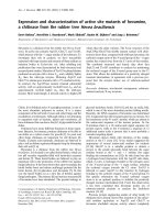
In the GoldenSpike dataset, there is a large difference
between NSB signal in C and S samples. For un-normalized
PM probes that have been summarized into probesets, empty
probesets are 50% brighter in the S samples compared to the
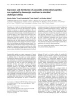
C samples (Figure 1a). The difference in NSB signal is also evi-
dent in low intensity FC = 1 and FC > 1 probesets, and we sug-
gest this difference is due to the different amounts of labeled
cRNA added to each hybridization.
The C and S samples in the GoldenSpike dataset have similar
amounts of total RNA hybridized to the Affymetrix chips but
have different amounts of labeled transcript. The S samples
have almost twice the amount of labeled cRNA hybridized to
each replicate chip as C samples (due to the 'spiked-in' tran-
scripts). For the samples to have the same amount of total
RNA hybridized, the C samples were supplemented with
unlabeled poly(C) RNA. As the cRNA in the C and S samples

are made from the same PCR amplification and labeling reac-
R126.4 Genome Biology 2007, Volume 8, Issue 6, Article R126 Schuster et al. />Genome Biology 2007, 8:R126
tion, the difference in the total amount of labeled RNA
hybridized to the chips is the most likely explanation for the
empty and low intensity probesets in the S samples being sig-
nificantly higher than in the C samples. Proper correction for
NSB would result in empty and FC = 1 probesets having a log2
difference of zero between C and S replicates.
MAS5 PM-MM is a poor model for estimating NSB
False positives for differentially expressed genes
The most common model for the removal of non-specific
binding signal is the MAS5 PM-MM model. In this model, the
MM probe intensity is an estimate for the non-specific bind-
ing of its partner PM probe. However, this model does not
seem to correct for non-specific binding as the intensities of
empty S probesets are still roughly 50% greater than empty
probesets in C samples (Figure 1b).
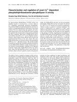
If NSB signal is not estimated correctly, then normalization
can potentially distort the analysis of the data. This is clearly
demonstrated by normalizing the GoldenSpike dataset with
the method recommended by Choe et al. [3] (the GoldenSpike
method) using all null probesets (empty and FC = 1) as a sub-
set for normalization. Normalization cannot compensate for
improper correction of NSB signal, and null-probeset nor-
malization will shift the log2 difference between empty
probesets towards zero, at the expense of low intensity FC = 1
probesets, which become down-regulated (Figure 2a). If only
FC = 1 probesets are used as a subset for normalization, then
the FC = 1 probesets behave as expected (log2 differences cen-
tered around zero), but the empty probesets are up-regulated

(Figure 2b). By comparing the number of probesets with q-
values (an estimate of FDRs) below 0.10 as calculated by the
Cyber-T method recommended in Choe et al. [3], the total
number of FPs is reduced by normalization using all null
probesets compared to FC = 1 probesets, but the number of
FC = 1 FPs is greater (Table 1).
P value distributions of null probesets
The q-value of a probeset is defined as an estimate of the pro-
portion of FPs among all probesets with equal or lower q-val-
ues. To calculate q-values, a test statistic is generated for the
data and for permutations of the data. The permutations are
based on randomly re-assigning the sample labels (for exam-
ple, given the six GoldenSpike RNA samples and three C/S
Plot of mean log2 difference versus mean log2 intensity (MA plot) of C and S samplesFigure 1
Plot of mean log2 difference versus mean log2 intensity (MA plot) of C and S samples. MA plots for the (a) PM-only and (b) MAS5 PM-MM summary
methods. Log2 differences greater than 0 imply that the average log2 intensity values in S samples are greater than C samples. Grey points represent
empty probesets, black points represent FC = 1 probesets, and red points represent 'differentially expressed' FC > 1 probesets. The green 'x' is located at
the mean log2 difference and mean log2 intensity of empty probesets.
(a) (b)
Mean log2 difference
-1.0 -0.5 0.0 0.5 1.0 1.5 2.0
Mean log2 intensity
0 5 10 15
Empty
FC=1
FC>1
Mean log2 difference
-1.0 -0.5 0.0 0.5 1.0 1.5 2.0
Mean log2 intensity
0 5 10 15

Empty
FC=1
FC>1
Genome Biology 2007, Volume 8, Issue 6, Article R126 Schuster et al. R126.5
comment reviews reports refereed researchdeposited research interactions information
Genome Biology 2007, 8:R126
replicates, there are nine permutations of sample labels that
do not match the 'correct' labeling), and for a particular test
statistic cutoff, the mean number of probesets called signifi-
cant after sample label permutation is an estimate of the
number of FPs for that cutoff value and used to calculate q-
values [11,15]. At a given test statistic, if 100 probesets are sig-
nificant when the sample labels are correct and on average 10
probesets are significant when the sample labels are per-
muted, then the estimate of FDR for that cutoff value (q-
value) is 0.10.
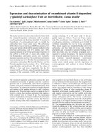
Proper estimation of q-values requires that null probesets
have a uniform distribution of P values [19], but in the Gold-
enSpike dataset, the differences in NSB results in many null
probesets having low P values. After NSB correction and nor-
malization, the log2 mean difference between null probesets
in C and S samples should be centered around zero and the P
values for null probesets should be uniformly distributed
between 0 and 1, but after MAS5 PM-MM correction, these
requirements are not met (Figures 2 and 3). This results in q-
values that considerably underestimate the true q-values
Plot of mean log2 difference versus mean log2 intensity (MA plot) showing FPsFigure 2
Plot of mean log2 difference versus mean log2 intensity (MA plot) showing FPs. MA plots are for probes normalized with the GoldenSpike method using
(a) all null probesets (empty and FC = 1) as a subset and (b) only FC = 1 probesets as a subset. In the plots, red spots represent FC > 1 probesets that
are called significantly differentially expressed (q < 0.1) by the modified Cyber-T method suggested by Choe et al. (that is, TPs). Pink spots represent FC >

1 false negatives. Grey symbols represent empty probesets that are not called significantly differentially expressed (true negatives), and blue symbols
represent empty probesets that are called significantly differentially expressed (FPs). Black symbols represent FC = 1 true negatives, and green symbols
represent FC = 1 FPs.
Table 1
False positives using the GoldenSpike MAS5 PM-MM methods
Total Null subset normalization FC = 1 subset normalization
Empty 10,104 487 1,729
FC = 1 2,495 251 180
FC > 1 1,284 1,015 1,057
All probesets with q-values below 0.10 based on the GoldenSpike normalizations and Cyber-T statistical analysis [3].
Mean log2 difference
-2 -1 0 1 2
Mean log2 intensity
0 2 4 6 8 10 12 14
Empty (TN)
FC=1 (TN)
FC>1 (TP)
(a)
Empty (FP)
FC=1 (FP)
FC>1 (FN)
Mean log2 difference
-2 -1 0 1 2
Mean log2 intensity
0 2 4 6 8 10 12 14
Empty (TN)
FC=1 (TN)
FC>1 (TP)
(b)
Empty (FP)

FC=1 (FP)
FC>1 (FN)
R126.6 Genome Biology 2007, Volume 8, Issue 6, Article R126 Schuster et al. />Genome Biology 2007, 8:R126
[3,16], and our analysis shows that at a 0.10 q-value cutoff,
the real q-value is 0.77 for FC = 1 probeset normalizations. We
suggest that to reduce the number of FPs, it is essential to
make a better estimate of NSB signal and/or to better detect
and remove all probesets that are not bound by their target
transcript. For example, if all empty probesets are removed
and the q-values are re-calculated, then a q-value of 0.10
would correspond to a true q-value of 0.28.
While the differences in NSB signal in C and S samples
account for a significant proportion of null probesets with low
P values, there are other issues that will effect the P value dis-
tribution of null probesets. A single C and S sample was gen-
erated and an aliquot from each sample was used to create
each replicate, and technical variation in the methods to gen-
erate each hybridization could result in subtle P values biases
if not accounted for in the statistical analysis. For example,
the mean raw PM values for FC = 1 probesets (1,898, 2,210
and 2,495 for C replicates, and 2,257, 1,803, and 2,466 for S
replicates) suggests different sized aliquots and possible pair-
ing between C and S replicates based on aliquot size. Also,
most fluidics stations can only hybridize four samples at one
time, and with six replicates, there might be two batches of
hybridizations. It is beyond the scope of this manuscript to
address all the possible sources of technical variation and
account for it in statistical models, as we have concentrated
on using the GoldenSpike dataset to infer the best methods to
correct NSB and have not used the dataset to evaluate statis-

tical methods. With only three replicates, it is also unlikely
that technical variation can be properly taken into account.
For example, analysis of the Latin Square spike-in experi-
ment (3 replicates of 14 samples with 42 spiked-in tran-
scripts) [4] revealed similar bias null probesets having low P
values bias for null probesets, even when the set of TPs was
expanded to include probesets that do not perfectly match the
spiked-in transcripts [20].
Probe sequence-dependent models for NSB correction
Having shown that PM-MM is a poor model for estimating
NSB signal, we tested if the non-specific binding signal could
be better modeled with the Zhang and Naef probe sequence-
dependent models for short oligonucleotide binding. To do
this, we used the GoldenSpike dataset at the level of the
probes rather than at the level of probesets and took great
care to align the probe sequences on the clones' sequences
when available. When there was no complete clone sequence,
we used the Drosophila Genome Release 4.0 [21] to pad the
missing sequence. To reduce any effect of promiscuity, we
used only empty probes that cannot be mapped to any clone,
even when up to six alignment errors are considered.
We tried to evaluate the success of two models describing
NSB of empty probes: a model based on Naef et al. [17] that
assumes that the affinity of a probe can be described as the
sum of the single nucleotide affinities across the probe. The
second model is based on Zhang's position-dependent-near-
est-neighbor (PDNN) model [18], in which the affinity of a
probe can be described by the sum of all nearest-neighbor di-
Histograms of P values for all null probesetsFigure 3
Histograms of P values for all null probesets. (a) The expected distribution of P values for null probesets is a uniform distribution between 0 and 1,

generated at random. The observed P value distribution after normalization using all (b) null probesets as a subset and (c) only FC = 1 probesets as a
subset are shown. MAS5 PM-MM was used for NSB correction, probes were normalized with the loess method, probes were summarized into probesets
with medianpolish, and P values were generated with Cyber-T.
0.0 0.2 0.4 0.6 0.8 1.0
0
500 1,000 1,500
2,000 2,500
3,000
0.0 0.2 0.4 0.6 0.8 1.0
0 500 1,000 1,500 2,000 2,500 3,000
0.0 0.2 0.4 0.6 0.8 1.0
0 500
1,000
1,500 2,000 2,500 3,000
(a)
P-values (random)
Frequency
(b)
P-values (null)
Frequency
(c)
P-values (FC=1)
Frequency
Genome Biology 2007, Volume 8, Issue 6, Article R126 Schuster et al. R126.7
comment reviews reports refereed researchdeposited research interactions information
Genome Biology 2007, 8:R126
nucleotides within a probe, but the influence of each di-
nucleotide is weighted depending on its position in the probe.
Both models are described in Materials and methods.
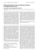
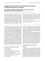
Figure 4a shows that the Naef model predicts a low affinity for

sequences with many adenines (A), while a sequence with
many cytosines (C) would have a high affinity. Using the Naef
model, fitted parameters for contributions of signal at each
position of a probe show a good consistency across all six RNA
samples (both C and S samples), and the model could reason-
ably reproduce the observed intensities of the empty probes
(Table 2).
The Zhang model predicts that probes with many GC di-
nucleotides would have a high signal especially if the GC di-
nucleotides are in the middle of the probe, as shown in Figure
4b,c. The fitted binding energy parameters derived for each
di-nucleotide in the six experiments are not as consistent as
the parameters fitted in the Naef model, but the parameters
fitted for the weights associated with each di-nucleotide posi-
tion are more consistent and confirm the importance of the
central part of the probe. Table 2 shows that the Zhang model
seems to predict the observations better than the Naef model
despite having fewer parameters, which apparently contra-
dicts a previous observation that di-nucleotide binding was
not the main effect in the binding [17]. However, our fitted
parameters for the Zhang model were significantly different
from those publicly available for four human chips and three
mouse chips.
We had also planned to use the GoldenSpike dataset to inves-
tigate the specific binding signal using models derived from
the Zhang and Naef models described above, taking
advantage of the fact that the clones' cRNA concentrations are
approximately known. Unfortunately, a detailed inspection of
the data suggested that there is a very high variability between
clone concentrations within a single PCR pool and we were

not able to use this dataset to model specific binding.
Comparing methods to generate probeset expression
values
Normalization methods
Our results emphasize that these sequence-based models are
powerful predictors of NSB, and should be applied before fur-
ther analysis, which agrees with previous observations [22].
Using BioConductor [10], we have combined various back-
ground and NSB correction methods to different normaliza-
tions and probeset-summarization methods to generate 300
different methods. When possible, we have normalized the
probes using the probes within FC = 1 probesets as a subset
for normalization; otherwise, all probes were used for nor-
malization. All probeset values were imported into R, and
Agreement between model parameters from the six replicatesFigure 4
Agreement between model parameters from the six replicates. (a) The Naef model scaled affinity parameters. They show good consistency, except for
the behavior of guanine near the probe attachment point (nucleotide position 25). (b) Zhang model scaled 'binding energy' parameters for each of the
three control samples (red circles, triangles and crosses) and for each of the three spike-in samples (green circles, triangles and crosses) for each di-
nucleotide pair. In addition, the average over the six samples is indicated with black circles and the average over the two sets of energy parameters
distributed for seven chip types distributed with Perfect Match [26] is indicated with black triangles and squares. The Zhang energy parameters are not as
consistent as the Naef parameters, especially for AG and GA di-nucleotides. (c) Zhang's weights parameters for the six experiments (red), their mean
(black line) and the average of the weights for the seven sets of weights (for non-specific and specific binding) distributed with the PDNN program (dotted
lines). The parameters refined here show a clear difference from the averages over the two sets of weights distributed with PDNN. In all cases, these
weights confirm the importance of the central part of the probe.
5 10152025
−2 −1 0 1 2
(a)
Nucleotide position
Scaled affinity
A

C
G
T
−2
−1 0 1 2
(b)
Di−nucleotide Position (Zhang Energies)
Scaled energy
GC
GT
AC
AT
CC
TC
GG
CT
GA
TT
AG
AA
TG
CG
CA
TA
●
●
●
●
●
●

●
●
●
●
●
●
●
●
●
●
●
●
●
●
●
●
●
●
●
●
●
●
●
●
●
●
●
●
●
●

●
●
●
●
●
●
●
●
●
●
●
●
5101520
0.0
0.2 0.4 0.6
0.8 1.0 1.2
1.4
(c)
Di−nucleotide position (Zhang Weights)
Scaled weight
R126.8 Genome Biology 2007, Volume 8, Issue 6, Article R126 Schuster et al. />Genome Biology 2007, 8:R126
Table 2
Results of fits on empty probes
C1 C2 C3 S1 S2 S3
Naef model 0.785 0.793 0.789 0.799 0.788 0.770
Zhang model 0.820 0.829 0.826 0.834 0.827 0.808
Naef scaling 0.782 0.790 0.788 0.796 0.787 0.766
Zhang scaling 0.821 0.830 0.828 0.835 0.830 0.810
The table shows the correlation coefficients between observed intensities for the empty probes on the three control (C) and spike-in (S)
experiments and the corresponding model predictions. The 'model' entries correspond to the correlation between observations and predicted

values for refinements of models, including the affinity, binding energy and weights parameters. The 'scaling' entries refer to the correlation between
the observation from the cross-validation set and the predicted values obtained by refining restricted models, where affinities, binding energies and
weights are kept constant at values obtained from the fits on the complete models (see Materials and methods). The agreement between the values
of correlation coefficients from both types of refinement suggests that the affinity, binding energy and weights parameters are general and do not
depend on the sequence or the experiment.
Normalization methodsFigure 5
Normalization methods. Diagram of methods used to create probeset expression values. When possible, probe-level normalization used FC = 1 probes as
a subset, and all probeset-level normalizations used FC = 1 probesets as a subset. For the normalization methods, additional parameters involve the use of
loess or spline to generate a normalization curve. See Materials and methods for more details. BG, background.
Probeset summarization
Medianpolish MAS AvgDiff affyPLM FARMSLiWon
g
NSB correction
Q
uantiles
no subset
Q
uantiles
FC=1 subset s
p
lines
Invariantset
median, s
p
lines
Invariantset
me an , s
p
lines
Probeset-level normalization

Loess VSN
Additional methods
Plier
GCRMA
RMA
External software
Perfect match
D
C
HIP
PM onl
y
model
D
C
HIP
PM/MM m odel
Probe-level normalization
No norm VSNConstant Loess
GC-NSBMAS5 PM-MMRMA BG only
Genome Biology 2007, Volume 8, Issue 6, Article R126 Schuster et al. R126.9
comment reviews reports refereed researchdeposited research interactions information
Genome Biology 2007, 8:R126
normalized using FC = 1 probesets as a subset. (see Figure 5
and Materials and methods for more details).
Similar to the analysis in [3], we have compared several meth-
ods to generate probeset expression values, but we have cho-
sen to evaluate each method based on the following criteria:
the estimation of fold changes for FC = 2 probesets, the ability
to separate true fold changes from false fold changes, the rate

of finding TPs versus the rate of finding FPs, and the differ-
ence between calculated q-values and true q-values. There are
too many methods to discuss individually, and we have lim-
ited the discussion to groups of methods that have the same
NSB correction method and/or same probe summary
method, as the choice of NSB correction and probe summary
method seem to have the biggest influence on performance.
Accuracy and precision
It has been previously observed that background correction
"appears to improve accuracy but, in general, worsen preci-
sion" [23], and various methods have been put forward to
measure accuracy and precision. As the concentration of each
transcript is not known but the exact fold change is known in
the GoldenSpike experiment, we have chosen the mean log2
fold change for the probesets that can be aligned to tran-
scripts with a two-fold difference (FC = 2) between C and S
samples to be a measure of accuracy (mean of 125 probesets
with the lowest P values as calculated by Cyber-T). As a meas-
ure of precision, we have taken 1% of FC = 1 and 1% of empty
probesets with the lowest P values. Ideally, the log2 fold
changes of FC = 2 probesets would be 1 and easily distin-
guished from fold changes of null probesets, as empty and FC
= 1 probesets are expected to have a log2 fold change of zero.
Methods using GC robust multichip average (RMA) NSB cor-
rection (GC-NSB) are the most sensitive and have the highest
estimate of FC = 2 but also tend to have the highest estimates
of null fold changes. Conversely, methods using RMA back-
ground correction are the most specific and have the lowest
FC = 2 fold change estimate but also have the lowest null fold
change estimates. However, the method of probe summary

and probeset-level normalization influences both the esti-
mate of FC = 2 fold changes and the difference between FC =
2 and null fold changes (Figure 6a,b).
Performance measured by AUC
While differences between FC = 2 and null probeset fold
changes are interesting, it is not a good measure of perform-
ance for separating truly differentially expressed genes from
FPs. To measure the performance of each method, we calcu-
lated the area under the ROC (AUC) using Cyber-T P values
as predictions. To allow a comparison of AUC measures based
on the presence or absence of transcript, we also made two
AUC calculations for each method, one using only probesets
with 'present' transcripts (FC > 1, FC = 1, and mixed) and one
using all probesets (FC > 1, FC = 1, mixed, and empty).
The use of empty probesets results in a drop of AUC perform-
ance, especially when only background correction and not
NSB correction is used, and this suggests that empty
probesets are a more significant source of FPs that bound FC
= 1 probesets. The best performing methods for probesets
with present transcripts use GC-NSB, affyPLM or median-
polish probe summary and variance stabilization normaliza-
tion (vsn) probeset-level normalization, but there is little
difference between MAS5 PM-MM and GC-NSB methods
when the probesets are normalized with the loess method
(Figure 6c).
It is also clear in Figure 6c that the GoldenSpike method
(called GOLD in the Figures) for combining the statistical
analysis of eight different normalization methods [3] does not
result in performance gains compared to individual MAS5
PM-MM normalization methods. In fact, the combined statis-

tical analysis tends to under-perform the four individual nor-
malization methods that use medianpolish probe summary.
True q-values
The AUC performance measure compares only the rate of
finding TPs and FPs, and high scoring methods may not be
appropriate for a proper analysis of the data. For example,
some of the methods with high AUC performance scores give
poor estimates of true q-values, and users may not be able to
distinguish TPs from FPs with a reasonable P value or q-value
because all probesets have very low P values (Figure 7). To put
the AUC performance measure into context, we calculated q-
values for every method and compared the actual q-values to
a calculated q-value of 0.10.
In general, methods that correct for NSB tend to have more
accurate q-values when considering all probesets and only
probesets with present transcripts, but the q-values gener-
ated with all probesets are very poor estimates of the true q-
value. The method that gave the most accurate measure of q-
values for probesets with present transcripts was the Golden-
Spike method, suggesting that combining statistical analyses
might be a method to extract more accurate estimates of q-
values (Figure 6d).
The AUC performance and true q-value comparisons high-
light how difficult it is to compare methods to find a 'best
method', and it is best left to the user to determine which is
the best method in the context of their experiment. However,
it is very clear that empty probesets contribute a significant
number of FPs and greatly distort q-value calculation in the
GoldenSpike dataset, and users should gauge the contribu-
tion of probesets with absent transcripts to estimated FDRs.

Performance is dependent on probeset intensity
There has been speculation that the best methods for normal-
ization are dependent on transcript concentrations [23,24].
We have attempted to address the issue by comparing AUC
performance (FC > 1 probesets as TPs, all null probesets as
R126.10 Genome Biology 2007, Volume 8, Issue 6, Article R126 Schuster et al. />Genome Biology 2007, 8:R126
FPs) and true q-value calculations using probeset intensities
as an approximation of transcript concentration. Probesets
were classified as unbound, low intensity, medium intensity
and high intensity. After removal of unbound probesets, the
remaining probesets were placed in categories based on the
mean log2 probeset expression value in control replicate sam-
ples from a range of methods used to generate probeset
expression values and each subset has the same number of FC
> 1 probesets. For each category, the cel files were masked to
remove all probes that were not part of the probeset category,
and probeset expression values were re-calculated. Perform-
ance measures were generated for expression values
generated from 'masked' cel files and from normalizations
using all probes, as there can be subtle but significant differ-
ences between the two methods (Figure 8).
Unbound probesets
We have defined unbound probesets as probesets that are
very unlikely to exhibit specific-binding signal (that is, empty
probesets and probesets that are specific for transcripts that
are too scarce to be detected). The default settings for the
MAS5 present/absent algorithm [7,25] are not stringent
enough to identify these probesets, as more than 25% of the
probesets classified as having present target transcripts are
Measures of performanceFigure 6

Measures of performance. (a) Plot of mean log2 fold changes for FC = 2, empty and FC = 1 probesets for all 300 methods to generate probeset
expression values. The mean was generated from the probesets with the lowest Cyber-T P values, the lowest 90% for TPs (125 out of 139 for FC = 2) and
the lowest 1% for FPs (101 out of 10,104 for empty; 25 out of 2,495 for FC = 1). (b) Plot of ratio of mean fold change of TPs (FC = 2) divided by mean fold
change of FPs (empty or FC = 1). (c) Plot of AUC scores for all probesets and for probesets that can be aligned to present transcripts (FC = 1, FC > 1 and
mixed probesets). TPs were FC > 1 probesets and mixed probesets that could be aligned to spiked-in transcripts. All other probesets are true negatives.
The plot also includes AUC scores using the FP rate of empty probesets to show which methods work best to reduce FDRs associated with present or
absent transcripts. (d) Plot of observed FDR (true q-value) based on the calculated q-values below 0.10 when considering only probesets with present
transcripts. To show the contribution of probesets with absent transcripts to FDRs, the plot also includes the observed FDR when all probesets are used.
0.2
0.4 0.6 0.8
1.0
1.2
1.4
●
●●
●
●
●
●
●
●
●●
●
●
●
●
●
●
●●
●

●
●
●
●
●
●●
●
●
●
●
●
●
●●
●●
●
●
●
●
●●
●
●
●
●
●
●
● ●
●
●
●
●

●
●
● ●
●
●
●
●
●
●
● ●
●
●
●
●
●
●
● ●
●
●
●
●
●
●
● ●
●
●
●
●
●
●

● ●
●
●
●
●
●
●
●●
●
●
●
●
●
●
●●
●
●
●
●
●
●
●●
●
●
●
●
●
●
●●
●

●
●
●
●
●
●●
●
●
●
●
●
●
●●
●
●
●
●
●
●
● ●
●
●
●
●
●
●
● ●
●
●
●

●
●
●
● ●
●
●
●
●
●
●
● ●
●
●
●
●
●
●
● ●
●
●
●
●
●
●
● ●
●
●
●
●
●

●
●●
●
●
●
●
●
●
●●
●
●
●
●
●
●
●●
●
●
●
●
●
●
●●
●
●
●
●
●
●
●●

●
●
●
●
●
●
●●
●
●
●
●
●
●
● ●
●
●
●
●
●
●
● ●
●
●
●
●
●
●
● ●
●
●

●
●
●
●
● ●
●
●
●
●
●
●
● ●
●
●
●
●
●
●
● ●
●
●
●
●
●
●
●
●
●
●
●

●
●
●
●
●
●
●
*
**
*
*
*
*
*
*
**
*
*
*
*
*
*
**
*
*
*
*
*
*
**

*
*
*
*
*
*
**
*
*
*
*
*
*
**
*
*
*
*
*
*
**
*
*
*
*
*
*
**
*
*

*
*
*
*
**
*
*
*
*
*
*
**
*
*
*
*
*
*
**
*
*
*
*
*
*
**
*
*
*
*

*
*
**
*
*
*
*
*
*
**
*
*
*
*
*
*
**
*
*
*
*
*
*
**
*
*
*
*
*
*

**
*
*
**
*
*
**
*
*
*
*
*
*
**
*
*
*
*
*
*
**
*
*
*
*
*
*
**
*
*

*
*
*
*
**
*
*
*
*
*
*
**
*
*
*
*
*
*
**
*
*
*
*
*
*
**
*
*
*
*

*
*
**
*
*
*
*
*
*
**
*
*
*
*
*
*
**
*
*
*
*
*
*
**
*
*
*
*
*
*

**
*
*
*
*
*
*
**
*
*
*
*
*
*
**
*
*
*
*
*
*
**
*
*
*
*
*
*
**
*

*
*
*
*
*
**
*
*
*
*
*
*
**
*
*
*
*
*
*
*
*
*
*
*
*
*
*
*
*
*

*
0.6 0.8
1.0
1.2
1.4
●
●●
●
●
●
●
●
●
●●
●
●
●
●
●
●
●●
●
●
●
●
●
●
●●
●
●

●
●
●
●
●●
●
●
●
●
●
●
●●
●
●
●
●
●
●
● ●
●
●
●
●
●
●
● ●
●
●
●
●

●
●
● ●
●
●
●
●
●
●
● ●
●
●
●
●
●
●
● ●
●
●
●
●
●
●
● ●
●
●
●
●
●
●

●●
●
●
●
●
●
●
●●
●
●
●
●
●
●
●●
●
●
●
●
●
●
●●
●
●
●
●
●
●
●●
●

●
●
●
●
●
●●
●
●
●
●
●
●
● ●
●
●
●
●
●
●
● ●
●
●
●
●
●
●
● ●
●
●
●

●
●
●
● ●
●
●
●
●
●
●
● ●
●
●
●
●
●
●
● ●
●
●
●
●
●
●
●●
●
●
●
●
●

●
●●
●
●
●
●
●
●
●●
●
●
●
●
●
●
●●
●
●
●
●
●
●
●●
●
●
●
●
●
●
●●

●
●
●
●
●
●
● ●
●
●
●
●
●
●
● ●
●
●
●
●
●
●
● ●
●
●
●
●
●
●
● ●
●
●

●
●
●
●
● ●
●
●
●
●
●
●
● ●
●
●
●
●
●
●
●
●
●
●
●
●
●
●
●
●
●
●

*
**
*
*
*
*
*
*
**
*
*
*
*
*
*
**
*
*
*
*
*
*
**
*
*
*
*
*
*
**

*
*
*
*
*
*
**
*
*
*
*
*
*
**
*
*
*
*
*
*
**
*
*
*
*
*
*
**
*
*

*
*
*
*
**
*
*
*
*
*
*
**
*
*
*
*
*
*
**
*
*
*
*
*
*
**
*
*
*
*

*
*
**
*
*
*
*
*
*
**
*
*
*
*
*
*
**
*
*
*
*
*
*
**
*
*
*
*
*
*

**
*
*
*
*
*
*
**
*
*
*
*
*
*
**
*
*
*
*
*
*
**
*
*
*
*
*
*
**
*

*
*
*
*
*
**
*
*
*
*
*
*
**
*
*
*
*
*
*
**
*
*
*
*
*
*
**
*
*
*

*
*
*
**
*
*
*
*
*
*
**
*
*
*
*
*
*
**
*
*
*
*
*
*
**
*
*
*
*
*

*
**
*
*
*
*
*
*
**
*
*
*
*
*
*
**
*
*
*
*
*
*
**
*
*
*
*
*
*
**

*
*
*
*
*
*
**
*
*
*
*
*
*
*
*
*
*
*
*
*
*
*
*
*
*
0.75 0.80 0.85 0.90
●
●
●●
●

●
●
●
●
●
●●
●
●
●
●
●
●
●●
●
●
●
●
●
●
●●
●
●
●
●
●
●
●●
●
●
●

●
●
●
●●
●
●
●
●
●
●
● ●
●
●
●
●
●
●
● ●
●
●
●
●
●
●
● ●
●
●
●
●
●

●
● ●
●
●
●
●
●
●
● ●
●
●
●
●
●
●
● ●
●
●
●
●
●
●
●●
●
●
●
●
●
●
●●

●
●
●
●
●
●
●●
●
●
●
●
●
●
●●
●
●
●
●
●
●
●●
●
●
●
●
●
●
●●
●
●

●
●
●
●
● ●
●
●
●
●
●
●
● ●
●
●
●
●
●
●
● ●
●
●
●
●
●
●
● ●
●
●
●
●

●
●
● ●
●
●
●
●
●
●
● ●
●
●
●
●
●
●
●●
●
●
●
●
●
●
●●
●
●
●
●
●
●

●●
●
●
●
●
●
●
●●
●
●
●
●
●
●
●●
●
●
●
●
●
●
●●
●
●
●
●
●
●
● ●
●

●
●
●
●
●
● ●
●
●
●
●
●
●
● ●
●
●
●
●
●
●
● ●
●
●
●
●
●
●
● ●
●
●
●

●
●
●
● ●
●
●
●
●
●
●
●
●
●
●
●
●
●
●
●
●
●
●
*
**
*
*
*
*
*
*