formulas and functions with microsoft excel 2003 phần 8 pdf

Use the DATEDIF function to determine all
friends younger than 30
You have the birth dates of your friends listed in a worksheet and
want to shade those who are currently younger than 30 years old.
Use the TODAY function to determine the actual date and the
DATEDIF function to calculate the exact age, then combine those
functions with conditional formatting.
4
To determine all friends younger than 30:
1. In a worksheet, enter data in cells A2:B10, as shown in
Figure 10-25.
2. Select cells A2:B10.
3. On the Format menu, click Conditional Formatting.
4. Select Formula Is and type the following formula:
=DATEDIF($B2,TODAY(),"Y")<30.
5. Click Format.
6. From the Patterns tab, select a color and click OK.
7. Click OK.
270
Chapter 10
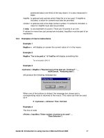
Figure 10-25
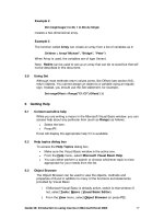
Use the MONTH and TODAY functions to find
birthdays in the current month
Use the same list from the previous tip to determine whose birth
-
day falls in the current month. Use the TODAY function to
determine the actual date and the MONTH function to compare the
month of everyone’s birthday with the current month, then com
-
bine those functions with conditional formatting.
4

To determine all friends whose birthday is in the current
month:
1. In cell D1 enter the formula TODAY().
2. Select cells A2:B10.
3. On the Format menu, click Conditional Formatting.
4. Select Formula Is and type the following formula:
=(MONTH(TODAY())=MONTH($B2)).
5. Click Format.
6. From the Patterns tab, select a color and click OK.
7. Click OK.
Conditional Formatting with Formulas 271
10
Figure 10-26
Use conditional formatting to border
summed rows
Enhance worksheets with this tip for placing a border on special
cells. The worksheet contains daily sales for different teams. Their
sales are summed up after a certain period to get a current status.
To enhance the visibility of each sum, we want to border it automat
-
ically through conditional formatting. Use a simple instruction as
the condition for conditional formatting and border the row of each
cell that meets the desired condition.
4
To border all rows containing a sum:
1. In a worksheet, enter data in cells A1:C11, as shown in Fig-
ure 10-27, and select the range A2:C11.
2. On the Format menu, click Conditional Formatting.
3. Select Formula Is and type the following formula:
=$B2="sum".

4. Click Format.
5. On the Border tab, click the bottom line in the Border field.
6. Select the color red from the Color drop-down box.
7. Click OK.
272
Chapter 10
Figure 10-27
Use the LEFT function in a product search
In this example, you need to find all the product numbers that con
-
tain the same first three characters. Enter in cell A2 the product
number as the search criteria and let Excel find each product that
corresponds to the same first three characters. The first three
characters of the numbers can be extracted by the LEFT function.
The name of the first product appears automatically in cell B2 with
the following formula: =VLOOKUP($A$2,$A$5:$B$15,2,FALSE).
Use a combination of the LEFT function and conditional formatting
to shade each cell that meets the desired condition.
4
To shade product numbers that meet the criteria:
1. In a worksheet, copy the data in cells A4:B15, as shown in
Figure 10-28, and select cells A5:B15.
2. On the Format menu, click Conditional Formatting.
3. Select Formula Is and type the following formula:
=LEFT($A5,3)=LEFT($A$2,3).
4. Click Format.
5. In the Patterns tab, select a color and click OK.
6. Click OK.
Conditional Formatting with Formulas 273
10

Figure 10-28
Use the AND function to detect empty rows
in a range
The last tip in this chapter marks all empty cells in a range. Use a
combination of the AND function and conditional formatting to
shade each cell that meets the desired condition.
4
To detect empty rows in a range:
1. In a worksheet, copy the data in cells A1:B12, as shown in
Figure 10-29, and select the range A2:B12.
2. On the Format menu, click Conditional Formatting.
3. Select Formula Is and type the following formula:
=AND($A3>($A2+1),$B3>($B2+1)).
4. Click Format.
5. From the Patterns tab, select a color and click OK.
6. Click OK.
274
Chapter 10
Figure 10-29
Chapter 11
Working with Array
Formulas
275
Use the ADDRESS, MAX, and ROW functions to
determine the last used cell
With this tip, we learn the definition of an array formula. Here, we
want to determine the last used cell in a range and shade it. Com
-
bine the ADDRESS, MAX, and ROW functions as described below
to get the desired result.

4
To determine the last used cell in a range and shade it:
1. In column A list any kind of numbers.
2. Select cell B2 and type the following array formula:
=ADDRESS(MAX((A2:A100<>"")*ROW(A2:A100)),1).
3. Press <Ctrl+Shift+Enter>.
4. Select cells A2:A11.
5. From the Format menu, select Conditional Formatting.
6. Select Formula Is and type the following formula:
=ADDRESS(ROW(),1)=$B$2.
7. Click Format.
8. In the Patterns tab, select a color and click OK.
9. Click OK.
Note: As shown in Figure 11-1, Excel automatically inserts
the combined functions, which are defined as an array
formula between the braces ({ and }). Use an array formula
to perform several calculations to generate a single result or
multiple results.
276 Chapter 11
Working with Array Formulas 277
11
Figure 11-1
Use the INDEX, MAX, ISNUMBER, and ROW
functions to find the last number in a column
Use the table from the previous tip and continue with array formu
-
las. Now we want to determine the last value in column A. Use a
combination of the INDEX, MAX, ISNUMBER, and ROW functions
inside an array formula to have the desired result displayed in cell
B2.

Don’t forget to enter the array formula by pressing
<Ctrl+Shift+Enter> to enclose it in braces.
4
To determine the last number in a column:
1. In column A list values or use the table from the previous
tip.
2. Select cell B2 and type the following array formula:
=INDEX(A:A,MAX(ISNUMBER(A1:A1000)*ROW
(A1:A1000))).
3. Press <Ctrl+Shift+Enter>.
278
Chapter 11
Figure 11-2
Use the INDEX, MAX, ISNUMBER, and COLUMN
functions to find the last number in a row
In this example, the last value in each row has to be determined
and copied to another cell. To do this, combine the INDEX, MAX,
ISNUMBER, and COLUMN functions in an array formula.
4
To determine the last number in a row:
1. Generate a table like that shown in Figure 11-3 using the
range A1:F6.
2. In cells A9:A13 enter numbers from 2 to 6.
3. Select cell B9 and type the following array formula:
=INDEX(2:2,MAX(ISNUMBER(2:2)*COLUMN(2:2))).
4. Press <Ctrl+Shift+Enter>.
5. Select cells B9:B13.
6. Select Fill and then Down from the Edit menu to retrieve
the last value in each of the remaining rows.
Working with Array Formulas 279

11
Figure 11-3
Use the MAX, IF, and COLUMN functions to
determine the last used column in a range
Now let’s determine the last used column in a defined range by
using an array formula. All columns in the range A1:X10 have to be
checked and the last used column is then shaded automatically.
Here we use the MAX, IF, and COLUMN functions in an array for
-
mula and combine them with conditional formatting.
4
To determine the last used column in a range:
1. Select cells A1:D10 and enter any numbers.
2. Select cell B12 and type the following array formula:
=MAX(IF(A1:X10<>"",COLUMN(A1:X10))).
3. Press <Ctrl+Shift+Enter>.
4. Select cells A1:X10.
5. On the Format menu, click Conditional Formatting.
6. Select Formula Is and type the following formula:
=$B$12=COLUMN(A1).
7. Click Format.
8. In the Patterns tab, select a color and click OK.
9. Click OK.
280
Chapter 11
Figure 11-4
Use the MIN and IF functions to find the lowest
non-zero value in a range
The sales for a fiscal year are recorded by month. During the year
the month with the lowest sales has to be determined. If the list

contains all sales from the year, we simply use the MIN function to
get the lowest value. However, if we want to find the lowest sales
sometime during the year and we don’t have sales figures available
for some of the months, we have to use the IF function to take care
of the zero values. Combine the MIN and IF functions in an array
formula and use conditional formatting to shade the lowest value.
4
To detect the lowest non-zero value in a range:
1. In cells A2:A13 list the months January through December.
2. In column B list some sales values down to row 7.
3. Select cell F2 and type the following array formula:
=MIN(IF(B1:B13>0,B1:B13)).
4. Press <Ctrl+Shift+Enter>.
5. Select cells B2:B13.
6. On the Format menu, click Conditional Formatting.
7. Select Formula Is and type the following formula:
=$F$2=B2.
8. Click Format.
9. In the Patterns tab, select a color and click OK.
10. Click OK.
Working with Array Formulas 281
11
282 Chapter 11
Figure 11-5
Use the AVERAGE and IF functions to calculate
the average of a range, taking zero values
into consideration
Normally Excel calculates the average of a range without consider
-
ing empty cells. Use this tip to calculate the correct average when

some values in a range are missing. As in the previous example, we
use the IF function to take care of the zero values. Combine the
AVERAGE and IF functions in an array formula to obtain the cor
-
rect average of all listed costs.
4
To calculate the average of a range, taking zero values into
consideration:
1. In cells A2:A13 list the months January through December.
2. In column B list monthly costs down to row 7.
3. Select cell E1 and type the following array formula:
=AVERAGE(IF($B$2:$B$13<>0,$B$2:$B$13)).
4. Press <Ctrl+Shift+Enter>.
Note: The result can be checked by selecting cells B2:B7.
Right-click in the Excel status bar and select the built-in
Average function instead of the usually displayed Sum.
Working with Array Formulas
283
11
Figure 11-6
Use the SUM and IF functions to sum values
with several criteria
To sum values in a list, the SUMIF function is normally used.
Unfortunately, it is not that easy to sum values with different crite
-
ria. Using a combination of different functions in an array formula is
once again the solution. Use the SUM and IF functions together to
take several criteria into consideration. In this example, we want to
sum all values of a list that match both the word “wood” in column
A and a value larger than 500 in column B. The result is displayed

in cell E2.
4
To sum special values with several criteria:
1. In cells A2:A11 enter materials like wood, aluminium, and
metal.
2. In cells B2:B11 list sizes from 100 to 1000.
3. In cells C2:C11 enter the corresponding costs.
4. Select cell E2 and type the following array formula:
=(SUM(IF(A2:A11="wood",IF(B2:B11>500,C2:
C11)))).
5. Press <Ctrl+Shift+Enter>.
284
Chapter 11
Figure 11-7
Use the INDEX and MATCH functions to search
for a value that matches two criteria
To search for a value that takes one or more criteria into consider
-
ation, use the INDEX and MATCH functions together. In this
example, the search criteria can be entered in cells E1 and F1.
Generate a search function using those two search criteria for the
range A2:C11, and return the result in cell E2.
4
To search for a special value considering two criteria:
1. In a worksheet, copy the data in cells A1:C11, as shown in
Figure 11-8.
2. Enter W46 as the first criterion in cell E1, and enter 1235
as the second criterion in cell F1.
3. Select cell E2 and type the following array formula:
=INDEX(C1:C11,MATCH(E1&F1,A1:A11&B1:

B11,0)).
4. Press <Ctrl+Shift+Enter>.
Working with Array Formulas 285
11
Figure 11-8
Use the SUM function to count values that
match two criteria
To count values in a list, normally the COUNTIF function is used.
Unfortunately, COUNTIF cannot be used to count when several cri
-
teria must be taken into consideration. However, it is possible to
get the desired result using an array formula. Use the SUM func
-
tion to consider several criteria. In this example, we count the rows
that contain the word “wood” in column A and have a size larger
than 500 in column B.
4
To count special values that match two criteria:
1. In cells A2:A11 list materials like wood, aluminium, and
metal.
2. In cells B2:B11 enter sizes from 100 to 1000.
3. In cells C2:C11 list the cost of each product.
4. Select cell E2 and type the following array formula:
=SUM((A2:A11="wood")*(B2:B11>500)).
5. Press <Ctrl+Shift+Enter>.
286
Chapter 11
Figure 11-9
Use the SUM function to count values that
match several criteria

In the previous example, we took two criteria into consideration.
Now let’s adapt that example for three criteria. Count all rows that
meet these criteria: The material is “wood” (column A), the size is
larger than 500 (column B), and the sales price is higher than
$5,000 (column C). To get the desired result, use an array formula
that takes care of all three criteria.
4
To count special values that match several criteria:
1. In cells A2:A11 enter materials like wood, aluminium, and
metal.
2. In cells B2:B11 list sizes from 100 to 1000.
3. In cells C2:C11 enter the sales price for each product.
4. Select cell E6 and type the following array formula:
=SUM((A2:A11="wood")*(B2:B11>500)*(C2:C11>
5000)).
5. Press <Ctrl+Shift+Enter>.
Working with Array Formulas 287
11
Figure 11-10
Use the SUM function to count numbers from
x to y
For this tip, we want to count all sales from $2500 to less than
$5000. As previously described, COUNTIF handles only one condi
-
tion. Use an array formula with the SUM function to get the correct
result here.
4
To count sales from $2500 to less than $5000:
1. In cells A2:B11 list the daily sales and dates.
2. Select cell D2 and type the following array formula:

=SUM((A2:A11>=2500)*(A2:A11<5000)).
3. Press <Ctrl+Shift+Enter>.
4. Select cells A2:B11.
5. On the Format menu, click Conditional Formatting.
6. Select Formula Is and type the following formula:
=AND($A2>=2500,$A2<5000).
7. Click Format.
8. In the Patterns tab, select a color and click OK.
9. Click OK.
Note: To sum all shaded sales, use the array formula
=(SUM(IF(A2:A11>=2500,IF(A2:A11<5000,A2:A11)))) and
press <Ctrl+Shift+Enter>.
288 Chapter 11
Figure 11-11
Use the SUM and DATEVALUE functions to count
today’s sales of a specific product
The table in Figure 11-12 contains a number of products sold on dif
-
ferent days. We want to count all sales of one specific product for
just one day. To handle dates this way, use the DATEVALUE func
-
tion, which converts a date represented by text to a serial number.
Use an array formula to count all the sales of one product for the
desired day.
4
To count today’s sales of a specific product:
1. In cells A2:A15 list dates.
2. In cells B2:B15 enter product numbers.
3. In cell E1 enter =TODAY().
4. Select cell E2 and type the following array formula:

=SUM((DATEVALUE("11/25/06")=$A$2:$A$15)*("K7
896"=$B$2:$B$15)).
5. Press <Ctrl+Shift+Enter>.
Working with Array Formulas 289
11
Figure 11-12
Use the SUM function to count today’s sales of
a specific product
This example is similar to the previous one, except the search cri
-
teria are variable. The array formula refers now to cells E1 and E2
and sums up all counted sales for one product on a specified date in
cell E4.
4
To count sales of a specific product for one day:
1. In cells A2:A15 list dates.
2. In cells B2:B15 enter product numbers.
3. Select cell E1 and enter the desired date to be considered
for counting.
4. Select cell E2 and select one product number.
5. Select cell E4 and type the following array formula:
=SUM((E1=$A$2:$A$15)*(E2=$B$2:$B$15)).
6. Press <Ctrl+Shift+Enter>.
290
Chapter 11
Figure 11-13
Use the SUM, OFFSET, MAX, IF, and ROW
functions to sum the last row in a dynamic list
Figure 11-14 shows a list that is updated constantly. The task here
is to determine the last row and sum up its entries. Use the MAX

and ROW functions to detect the last used row, then sum that row
with help from the SUM and OFFSET functions. Combine all these
functions in one array formula and assign the calculated result to
cell H2.
4
To sum the last row in a dynamic list:
1. In cells A2:A11 enter dates.
2. In cells B2:F11 list numbers for each team.
3. Select cell H2 and type the following array formula:
=SUM(OFFSET(B1:F1,MAX(IF(B1:F100<>"",
ROW(1:100)))-1,)).
4. Press <Ctrl+Shift+Enter>.
Note: Check the result by selecting cells B11:F11. Click with
the right mouse button on the status bar at the bottom of the
Excel window and select the Sum function.
Working with Array Formulas 291
11
Figure 11-14
Use the SUM, MID, and COLUMN functions to
count specific characters in a range
In this example, we want to count specific characters that appear in
a range. Use the MID function to extract each character from the
cells, then define the range to be searched using the COLUMN
function. The SUM function counts the result. Combine all these
functions into one array formula.
4
To count certain characters in a range:
1. In cells A2:A11 list IP addresses.
2. Insert in any cells one or more characters like x or xxx.
3. Select cell D2 and type the following array formula:

=SUM((MID(A1:A11,COLUMN(1:1),3)="xxx")*1).
4. Press <Ctrl+Shift+Enter>.
5. Select cell D3 and type the following array formula:
=SUM((MID(A1:A11,COLUMN(1:1),1)="x")*1).
6. Press <Ctrl+Shift+Enter>.
292
Chapter 11
Figure 11-15
Use the SUM, LEN, and SUBSTITUTE functions to
count the occurrences of a specific word in a
range
In this example, we want to count how many times a specific word
appears in a range. Use the SUM, SUBSTITUTE, and LEN func
-
tions in one array formula to do this. Enter the criterion in cell C1
and let Excel display the result of counting in cell C2.
4
To count the occurrences of a specific word in a range:
1. In cells A2:A11 type any text but enter the word test at
least once.
2. In cell C1 enter the word test.
3. Select cell C2 and type the following array formula:
=SUM((LEN(A1:A10)-LEN(SUBSTITUTE(A1:A10,
C1,"")))/LEN(C1)).
4. Press <Ctrl+Shift+Enter>.
5. Select cells A2:A10.
6. On the Format menu, click Conditional Formatting.
7. Select Formula Is and type the following formula:
=$C$1=A1.
8. Click Format.

9. In the Patterns tab, select a color and click OK.
10. Click OK.
Working with Array Formulas 293
11
294 Chapter 11
Figure 11-16