Microsoft Excel 2010: Data Analysis and Business Modeling phần 2 pot
Bạn đang xem bản rút gọn của tài liệu. Xem và tải ngay bản đầy đủ của tài liệu tại đây (947.2 KB, 67 trang )
57
Chapter 8
Evaluating Investments by Using Net
Present Value Criteria
Questions answered in this chapter:
■
What is net present value (NPV)?
■
How do I use the Excel NPV function?
■
How can I compute NPV when cash ows are received at the beginning of a year or in
the middle of a year?
■
How can I compute NPV when cash ows are received at irregular intervals?
Consider the following two investments, whose cash ows are listed in the le NPV.xlsx and
shown in Figure 8-1.
■
Investment 1 requires a cash outow of $10,000 today and $14,000 two years from
now. One year from now, this investment will yield $24,000.
■
Investment 2 requires a cash outow of $6,000 today and $1,000 two years from now.
One year from now, this investment will yield $8,000.
Which is the better investment? Investment 1 yields total cash ow of $0, whereas Investment
2 yields a total cash ow of $1,000. At rst glance, Investment 2 appears to be better. But
wait a minute. Most of the cash outow for Investment 1 occurs two years from now, while
most of the cash outow for Investment 2 occurs today. Spending $1 two years from now
doesn’t seem as costly as spending $1 today, so maybe Investment 1 is better than rst
appears. To determine which investment is better, you need to compare the values of cash
ows received at different points in time. That’s where the concept of net present value
proves useful.
FIGURE 8-1 To determine which investment is better, you need to calculate net present value.
58 Microsoft Excel 2010: Data Analysis and Business Modeling
Answers to This Chapter’s Questions
What is net present value?
The net present value (NPV) of a stream of cash ow received at different points in time is
simply the value measured in today’s dollars. Suppose you have $1 today and you invest this
dollar at an annual interest rate of r percent. This dollar will grow to 1+r dollars in the rst
year, (1+r)
2
dollars in two years, and so on. You can say, in some sense, that $1 today equals
$(1+r) a year from now and $(1+r)
2
two years from now. In general, you can say that $1 today
is equal to $(1+r)
n
n years from now. As an equation, this calculation can be expressed as
follows:
$1 now=$(1+r)
n
received n years from now
If you divide both sides of this equation by (1+r)
n
, you get the following important result:
1/(1+r)
n
now=$1 received n years from now
This result tells you how to compute (in today’s dollars) the NPV of any sequence of cash
ows. You can convert any cash ow to today’s dollars by multiplying the cash ow received
n years from now (n can be a fraction) by 1/(1+r)
n
.
You then add up the value of the cash ows (in today’s dollars) to nd the investment’s NPV.
Let’s assume r is equal to 0.2. You could calculate the NPV for the two investments we’re
considering as follows:
24,000
(1 + 0.20)
1
= $277.78
–14,000
(1 + 0.20)
2
= Investment1NPV = –10,000 +
+
8,000
(1 + 0.20)
1
= $–27.78
–1,000
(1 + 0.20)
2
= Investment2NPV = –6,000 +
+
On the basis of NPV, Investment 1 is superior to Investment 2. Although total cash ow
for Investment 2 exceeds total cash ow for Investment 1, Investment 1 has a better NPV
because a greater proportion of Investment 1’s negative cash ow comes later, and the
NPV criterion gives less weight to cash ows that come later. If you use a value of .02 for
r, Investment 2 has a larger NPV because when r is very small, later cash ows are not dis-
counted as much, and NPV returns results similar to those derived by ranking investments
according to total cash ow.
Chapter 8 Evaluating Investments by Using Net Present Value Criteria 59
Note I randomly chose the interest rate r=0.2, skirting the issue of how to determine an
appropriate value of r. You need to study nance for at least a year to understand the issues
involved in determining an appropriate value for r. The appropriate value of r used to compute
NPV is often called the company’s cost of capital. Sufce it to say that most U.S. companies use
an annual cost of capital between 0.1 (10 percent) and 0.2 (20 percent). If the annual interest rate
is chosen according to accepted nance practices, projects with NPV>0 increase the value of a
company, projects with NPV<0 decrease the value of a company, and projects with NPV=0 keep
the value of a company unchanged. A company should (if it had unlimited investment capital)
invest in every available investment having positive NPV.
To determine the NPV of Investment 1 in Excel, I rst assigned the range name r_ to the in-
terest rate (located in cell C3). I then copied the Time 0 cash ow from C5 to C7. I determined
the NPV for Investment 1’s Year 1 and Year 2 cash ows by copying from D7 to E7 the for-
mula D5/(1+r_)^D$4. The caret symbol (^), located over the number 6 on the keyboard, raises
a number to a power. In cell A5, I computed the NPV of Investment 1 by adding the NPV of
each year’s cash ow with the formula SUM(C7:E7). To determine the NPV for Investment 2, I
copied the formulas from C7:E7 to C8:E8 and from A5 to A6.
How do I use the Excel NPV function?
The Excel NPV function uses the syntax NPV(rate,range of cells). This function determines the
NPV for the given rate of the cash ows in the range of cells. The function’s calculation as-
sumes that the rst cash ow is one period from now. In other words, entering the formula
NPV(r_,C5:E5) will not determine the NPV for Investment 1. Instead, this formula (entered
in cell C14) computes the NPV of the following sequence of cash ows: –$10,000 a year
from now, $24,000 two years from now, and –$14,000 three years from now. Let’s call this
Investment 1 (End of Year). The NPV of Investment 1 (End of Year) is $231.48. To compute
the actual cash NPV of Investment 1, I entered the formula C7+NPV(r_,D5:E5) in cell C11. This
formula does not discount the Time 0 cash ow at all (which is correct because Time 0 cash
ow is already in today’s dollars), but rst multiplies the cash ow in D5 by 1/1.2 and then
multiplies the cash ow in E5 by 1/1.2
2
.
The formula in cell C11 yields the correct NPV of Investment 1, $277.78.
How can I compute NPV when cash ows are received at the beginning of a year or in the
middle of a year?
To use the NPV function to compute the net present value of a project whose cash ows al-
ways occur at the beginning of a year, you can use the approach I described to determine the
NPV of Investment 1: separate out the Year 1 cash ow and apply the NPV function to the
remaining cash ows. Alternatively, observe that for any year n, $1 received at the beginning
60 Microsoft Excel 2010: Data Analysis and Business Modeling
of year n is equivalent to $(1+r) received at the end of year n. Remember that in one year, a
dollar will grow by a factor (1+r). Thus, if you multiply the result obtained with the NPV func-
tion by (1+r), you can convert the NPV of a sequence of year-end cash ows to the NPV of a
sequence of cash ows received at the beginning of the year. You can also compute the NPV
of Investment 1 in cell D11 with the formula (1+r_)*C14. Of course, you again obtain an NPV
of $277.78.
Now suppose the cash ows for an investment occur in the middle of each year. For an orga-
nization that receives monthly subscription revenues, you can approximate the 12 monthly
revenues received during a given year as a lump sum received in the middle of the year. How
can you use the NPV function to determine the NPV of a sequence of mid-year cash ows?
For any Year n,
$ 1 + r
received at the end of Year n is equivalent to $1 received at the middle of Year n because in
half a year $1 will grow by a factor of
1 + r
If you assume the cash ows for Investment 1 occur mid year, you can compute the NPV of
the mid-year version of Investment 1 in cell C17 with the formula SQRT(1+r_)*C14. You obtain
a value of $253.58.
How can I compute NPV when cash ows are received at irregular intervals?
Cash ows often occur at irregular intervals, which makes computing the NPV or internal rate
of return (IRR) of these cash ows more difcult. Fortunately, the Excel XNPV function makes
computing the NPV of irregularly timed cash ows a snap.
The XNPV function uses the syntax XNPV(rate,values,dates). The rst date listed must be
the earliest, but other dates need not be listed in chronological order. The XNPV function
computes the NPV of the given cash ows assuming the current date is the rst date in the
sequence. For example, if the rst listed date is 4/08/13, the NPV is computed in April 8, 2013
dollars.
To illustrate the use of the XNPV function, look at the example on the NPV as of rst date
worksheet in the le XNPV.xlsx, which is shown in Figure 8-2. Suppose that on April 8, 2013,
you paid out $900. Later you receive the following amounts:
■
$300 on August 15, 2013
■
$400 on January 15, 2014
■
$200 on June 25, 2014
■
$100 on July 3, 2015
Chapter 8 Evaluating Investments by Using Net Present Value Criteria 61
If the annual interest rate is 10 percent, what is the NPV of these cash ows? I entered
the dates (in Excel date format) in D3:D7 and the cash ows in E3:E7. Entering the formula
XNPV(A9,E3:E7,D3:D7) in cell D11 computes the project’s NPV in April 8, 2013 dollars because
that is the rst date listed. This project would have an NPV, in April 8, 2013 dollars, of $20.63.
FIGURE 8-2 Using the XNPV function.
The computations performed by the XNPV function are as follows:
1. Compute the number of years after April 8, 2013, that each date occurred. (I did this in
column F.) For example, August 15 is 0.3534 years after April 8.
2. Discount cash ows at the rate 1/(1+rate)
years after
.
For example, the August 15, 2013 cash ow is discounted by
1
(1 + 0.1)
3534
= 0.967
3. Sum up in cell E11 overall cash ows: (cash ow value)*(discount factor).
Suppose that today’s date is actually July 11, 2010. How would you compute the NPV of an
investment in today’s dollars? Simply add a row with today’s date and 0 cash ow and include
this row in the range for the XNPV function. (See Figure 8-3 and the Today worksheet.) The
NPV of the project in today’s dollars is $15.88.
FIGURE 8-3 NPV converted to today’s dollars.
I’ll close by noting that if a cash ow is left blank, the NPV function ignores both the cash
ow and the period. If a cash ow is left blank, the XNPV function returns a #NUM error.
62 Microsoft Excel 2010: Data Analysis and Business Modeling
Problems
1. An NBA player is to receive a $1,000,000 signing bonus today and $2,000,000 one year,
two years, and three years from now. Assuming r=0.10 and ignoring tax considerations,
would he be better off receiving $6,000,000 today?
2. A project has the following cash ows:
Now One year from now Two years from now Three years from now
–$4 million $4 million $4 million –$3 million
If the company’s cost of capital is 15 percent, should it proceed with the project?
3. Beginning one month from now, a customer will pay his Internet provider $25 per
month for the next ve years. Assuming all revenue for a year is received at the middle
of a year, estimate the NPV of these revenues. Use r=0.15.
4. Beginning one month from now, a customer will pay $25 per month to her Internet
provider for the next ve years. Assuming all revenue for a year is received at the
middle of a year, use the XNPV function to obtain the exact NPV of these revenues. Use
r=0.15.
5. Consider the following set of cash ows over a four-year period. Determine the NPV of
these cash ows if r=0.15 and cash ows occur at the end of the year.
Year 1 2 3 4
-$600 $550 -$680 $1,000
6. Solve Problem 5 assuming cash ows occur at the beginning of each year.
7. Consider the following cash ows:
Date Cash ow
12/15/01 –$1,000
1/11/02 $300
4/07/03 $600
7/15/04 $925
If today is November 1, 2001, and r=0.15, what is the NPV of these cash ows?
8. After earning an MBA, a student will begin working at an $80,000-per-year job on
September 1, 2005. She expects to receive a 5 percent raise each year until she retires
on September 1, 2035. If the cost of capital is 8 percent a year, determine the total
present value of her before-tax earnings.
9. Consider a 30-year bond that pays $50 at the end of Years 1–29 and $1,050 at the end
of Year 30. If the appropriate discount rate is 5 percent per year, what is a fair price for
this bond?
63
Chapter 9
Internal Rate of Return
Questions answered in this chapter:
■
How can I nd the IRR of cash ows?
■
Does a project always have a unique IRR?
■
Are there conditions that guarantee a project will have a unique IRR?
■
If two projects each have a single IRR, how do I use the projects’ IRRs?
■
How can I nd the IRR of irregularly spaced cash ows?
■
What is the MIRR and how do I compute it?
The net present value (NPV) of a sequence of cash ows depends on the interest rate (r)
used. For example, if you consider cash ows for Projects 1 and 2 (see the worksheet IRR in
the le IRR.xlsx, shown in Figure 9-1), you nd that for r=0.2, Project 2 has a larger NPV, and
for r=0.01, Project 1 has a larger NPV. When you use NPV to rank investments, the outcome
can depend on the interest rate. It is the nature of human beings to want to boil everything
in life down to a single number. The internal rate of return (IRR) of a project is simply the
interest rate that makes the NPV of the project equal to 0. If a project has a unique IRR, the
IRR has a nice interpretation. For example, if a project has an IRR of 15 percent, you receive
an annual rate of return of 15 percent on the cash ow you invested. In this chapter’s exam-
ples, you’ll nd that Project 1 has an IRR of 47.5 percent, which means that the $400 invested
at Time 1 is yielding an annual rate of return of 47.5 percent. Sometimes, however, a project
might have more than one IRR or even no IRR. In these cases, speaking about the project’s
IRR is useless.
FIGURE 9-1 Example of the IRR function.
64 Microsoft Excel 2010: Data Analysis and Business Modeling
Answers to This Chapter’s Questions
How can I nd the IRR of cash ows?
The IRR function calculates internal rate of return. The function has the syntax
IRR(range of cash ows,[guess]), where guess is an optional argument. If you do not enter a
guess for a project’s IRR, Excel begins its calculations with a guess that the project’s IRR is
10 percent and then varies the estimate of the IRR until it nds an interest rate that makes
the project’s NPV equal 0 (the project’s IRR). If Excel can’t nd an interest rate that makes
the project’s NPV equal 0, Excel returns #NUM. In cell B5, I entered the formula IRR(C2:I2) to
compute Project 1’s IRR. Excel returns 47.5 percent. Thus, if you use an annual interest rate of
47.5 percent, Project 1 will have an NPV of 0. Similarly, you can see that Project 2 has an IRR
of 80.1 percent.
Even if the IRR function nds an IRR, a project might have more than one IRR. To check
whether a project has more than one IRR, you can vary the initial guess of the project’s IRR
(for example, from –90 percent to 90 percent). I varied the guess for Project 1’s IRR by copy-
ing from B8 to B9:B17 the formula IRR($C$2:$I$2,A8). Because all the guesses for Project 1’s
IRR yield 47.5 percent, I can be fairly condent that Project 1 has a unique IRR of 47.5 percent.
Similarly, I can be fairly condent that Project 2 has a unique IRR of 80.1 percent.
Does a project always have a unique IRR?
In the worksheet Multiple IRR in the le IRR.xlsx (see Figure 9-2), you can see that Project 3
(cash ows of –20, 82, –60, 2) has two IRRs. I varied the guess about Project 3’s IRR from –90
percent to 90 percent by copying from C8 to C9:C17 the formula IRR($B$4:$E$4,B8).
FIGURE 9-2 Project with more than one IRR.
Note that when a guess is 30 percent or less, the IRR is –9.6 percent. For other guesses, the
IRR is 216.1 percent. For both these interest rates, Project 3 has an NPV of 0.
Chapter 9 Internal Rate of Return 65
In the worksheet No IRR in the le IRR.xlsx (shown in Figure 9-3), you can see that no matter
what guess you use for Project 4’s IRR, you receive the #NUM message. This message
indicates that Project 4 has no IRR.
When a project has multiple IRRs or no IRR, the concept of IRR loses virtually all meaning.
Despite this problem, however, many companies still use IRR as their major tool for ranking
investments.
FIGURE 9-3 Project with no IRR.
Are there conditions that guarantee a project will have a unique IRR?
If a project’s sequence of cash ows contains exactly one change in sign, the project is
guaranteed to have a unique IRR. For example, for Project 2 in the worksheet IRR, the sign of
the cash ow sequence is – + + + + +. There is only one change in sign (between Time 1 and
Time 2), so Project 2 must have a unique IRR. For Project 3 in the worksheet Multiple IRR, the
signs of the cash ows are – + – +. Because the sign of the cash ows changes three times,
a unique IRR is not guaranteed. For Project 4 in the worksheet No IRR, the signs of the cash
ows are + – +. Because the signs of the cash ows change twice, a unique IRR is not guaran-
teed in this case either. Most capital investment projects (such as building a plant) begin with
a negative cash ow followed by a sequence of positive cash ows. Therefore, most capital
investment projects do have a unique IRR.
If two projects each have a single IRR, how do I use the projects’ IRRs?
If a project has a unique IRR, you can state that the project increases the value of the
company if and only if the project’s IRR exceeds the annual cost of capital. For example, if the
cost of capital for a company is 15 percent, both Project 1 and Project 2 would increase the
value of the company.
66 Microsoft Excel 2010: Data Analysis and Business Modeling
Suppose two projects are under consideration (both having unique IRRs), but you can under-
take at most one project. It’s tempting to believe that you should choose the project with the
larger IRR. To illustrate that this belief can lead to incorrect decisions, look at Figure 9-4 and
the Which Project worksheet in IRR.xlsx. Project 5 has an IRR of 40 percent, and Project 6 has
an IRR of 50 percent. If you rank projects based on IRR and can choose only one project, you
would choose Project 6. Remember, however, that a project’s NPV measures the amount of
value the project adds to the company. Clearly, Project 5 will (for virtually any cost of capital)
have a larger NPV than Project 6. Therefore, if only one project can be chosen, Project 5 is
it. IRR is problematic because it ignores the scale of the project. Whereas Project 6 is better
than Project 5 on a per-dollar-invested basis, the larger scale of Project 5 makes it more valu-
able to the company than Project 6. IRR does not reect the scale of a project, whereas NPV
does.
FIGURE 9-4 IRR can lead to an incorrect choice of which project to pursue.
How can I nd the IRR of irregularly spaced cash ows?
Cash ows occur on actual dates, not just at the start or end of the year. The
XIRR function
has the syntax XIRR(cash ow, dates, [guess]). The XIRR function determines the IRR of a
sequence of cash ows that occur on any set of irregularly spaced dates. As with the IRR
function, guess is an optional argument. For an example of how to use the XIRR function,
look at Figure 9-5 and worksheet XIRR of the le IRR.xlsx.
FIGURE 9-5 Example of the XIRR function.
The formula XIRR(F4:F7,E4:E7) in cell D9 shows that the IRR of Project 7 is -48.69 percent.
What is the MIRR and how do I compute it?
In many situations the rate at which a company borrows funds is different from the rate
at which the company reinvests funds. IRR computations implicitly assume that the rate at
which a company borrows and reinvests funds is equal to the IRR. If we know the actual rate
at which we borrow money and the rate at which we can reinvest money, then the modied
internal rate of return (MIRR) function computes a discount rate that makes the NPV of all
Chapter 9 Internal Rate of Return 67
our cash ows (including paying back our loan and reinvesting our proceeds at the given
rates) equal to 0. The syntax of MIRR is MIRR(cash ow values,borrowing rate,reinvestment
rate).
A nice thing about MIRR is that it is always unique. Figure 9-6 in worksheet MIRR of
le IRR.xls contains an example of MIRR. Suppose you borrow $120,000 today and receive
the following cash ows: Year 1: $39,000, Year 2: $30,000, Year 3: $21,000, Year 4: $37,000,
Year 5: $46,000. Assume you can borrow at 10 percent per year and reinvest your prots at
12 percent per year.
After entering these values in cells E7:E12 of worksheet MIRR, you can nd the MIRR in cell
D15 with the formula MIRR(E7:E12,E3,E4). Thus, this project has an MIRR of 12.61 percent. In
cell D16 I computed the actual IRR of 13.07 percent.
FIGURE 9-6 Example of the MIRR function.
I’ll close by noting that if a cash ow is left blank, the IRR function ignores both the cash ow
and the period. If a cash ow is left blank, the IRR function will return a #NUM error.
Problems
1. Compute all IRRs for the following sequence of cash ows:
Year 1 Year 2 Year 3 Year 4 Year 5 Year 6 Year 7
–$10,000 $8,000 $1,500 $1,500 $1,500 $1,500 –$1,500
2. Consider a project with the following cash ows. Determine the project’s IRR. If the
annual cost of capital is 20 percent, would you undertake this project?
Year 1 Year 2 Year 3
–$4,000 $2,000 $4,000
68 Microsoft Excel 2010: Data Analysis and Business Modeling
3. Find all IRRs for the following project:
Year 1 Year 2 Year 3
$100 –$300 $250
4. Find all IRRs for a project having the given cash ows on the listed dates.
1/10/2003 7/10/2003 5/25/2004 7/18/2004 3/20/2005 4/1/2005 1/10/2006
–$1,000 $900 $800 $700 $500 $500 $350
5. Consider the following two projects, and assume a company’s cost of capital is 15 per-
cent. Find the IRR and NPV of each project. Which projects add value to the company?
If the company can choose only a single project, which project should it choose?
Year 1 Year 2 Year 3 Year 4
Project 1 –$40 $130 $19 $26
Project 2 –$80 $36 $36 $36
6. Twenty-ve-year-old Meg Prior is going to invest $10,000 in her retirement fund at
the beginning of each of the next 40 years. Assume that during each of the next 30
years Meg will earn 15 percent on her investments and during the last 10 years before
she retires, her investments will earn 5 percent. Determine the IRR associated with her
investments and her nal retirement position. How do you know there will be a unique
IRR? How would you interpret the unique IRR?
7. Give an intuitive explanation of why Project 6 (on the worksheet Which Project in the
le IRR.xlsx) has an IRR of 50 percent.
8. Consider a project having the following cash ows:
Year 1 Year 2 Year 3
–$70,000 $12,000 $15,000
Try to nd the IRR of this project without simply guessing. What problem arises? What
is the IRR of this project? Does the project have a unique IRR?
9. For the cash ows in Problem 1, assume you can borrow at 12 percent per year and
invest prots at 15 percent per year. Compute the project’s MIRR.
10. Suppose today that you paid $1,000 for the bond described in Problem 9 of Chapter 8,
“Evaluating Investments by Using Net Present Value Criteria.” What would be the
bond’s IRR? A bond’s IRR is often called the yield of the bond.
69
Chapter 10
More Excel Financial Functions
Questions answered in this chapter:
■
You are buying a copier. Would you rather pay $11,000 today or $3,000 a year for ve
years?
■
If at the end of each of the next 40 years I invest $2,000 a year toward my retirement
and earn 8 percent a year on my investments, how much will I have when I retire?
■
I am borrowing $10,000 for 10 months with an annual interest rate of 8 percent. What
are my monthly payments? How much principal and interest am I paying each month?
■
I want to borrow $80,000 and make monthly payments for 10 years. The maximum
monthly payment I can afford is $1,000. What is the maximum interest rate I can
afford?
■
If I borrow $100,000 at 8 percent interest and make payments of $10,000 per year, how
many years will it take me to pay back the loan?
When we borrow money to buy a car or house, we always wonder if we are getting a good
deal. When we save for retirement, we are curious how large a nest egg we’ll have when we
retire. In our daily work and personal lives, nancial questions similar to these often arise.
Knowledge of the Excel PV, FV, PMT, PPMT, IPMT, CUMPRINC, CUMIPMT, RATE, and NPER
functions makes it easy to answer these types of questions.
Answers to This Chapter’s Questions
You are buying a copier Would you rather pay $11,000 today or $3,000 a year for
ve years?
The key to answering this question is being able to value the annual payments of $3,000 per
year. Assume the cost of capital is 12 percent per year. You could use the NPV function to
answer this question, but the Excel PV function provides a much quicker way to solve it. A
stream of cash ows that involves the same amount of cash outow (or inow) each period
is called an annuity. Assuming that each period’s interest rate is the same, you can easily
value an annuity by using the Excel PV function. The PV function returns the value in today’s
dollars of a series of future payments, under the assumption of periodic, constant payments
and a constant interest rate. The syntax of the PV function is PV(rate,#per,[pmt],[fv],[type]),
where pmt, fv, and type are optional arguments.
70 Microsoft Excel 2010: Data Analysis and Business Modeling
Note When working with Microsoft Excel nancial functions, I use the following conventions for
the signs of pmt (payment) and fv (future value): money received has a positive sign and money
paid out has a negative sign.
■
Rate is the interest rate per period. For example, if you borrow money at 6 percent
per year and the period is a year, then rate=0.06. If the period is a month, then
rate=0.06/12=0.005.
■
#per is the number of periods in the annuity. For our copier example, #per=5. If
payments on the copier are made each month for ve years, then #per=60. Your rate
must, of course, be consistent with #per. That is, if #per implies a period is a month,
you must use a monthly interest rate; if #per implies a period is a year, you must use an
annual interest rate.
■
Pmt is the payment made each period. For our copier example, pmt=-$3,000. A
payment has a negative sign, whereas money received has a positive sign. At least one
of pmt or fv must be included.
■
Fv is the cash balance (or future value) you want to have after the last payment is made.
For our copier example, fv=0. For example, if you want to have a $500 cash balance
after the last payment, then fv=$500. If you want to make an additional $500 payment
at the end of a problem fv=–$500. If fv is omitted, it is assumed to equal 0.
■
Type is either 0 or 1 and indicates when payments are made. When type is omitted or
equal to 0, payments are made at the end of each period. When type=1, payments are
made at the beginning of each period. Note that you may also write True instead of 1
and False instead of 0 in all functions discussed in this chapter.
Figure 10-1 (see the worksheet PV of le the Excelnfunctions.xlsx) indicates how to solve our
copier problem.
FIGURE 10-1 Example of the PV function.
Chapter 10 More Excel Financial Functions 71
In cell B3 I computed the present value of paying $3,000 at the end of each year for ve
years with a 12 percent cost of capital by using the formula =PV(0.12,5,–3000,0,0). Excel
returns an NPV of $10,814.33. By omitting the last two arguments, I obtained the same
answer with the formula =PV(0.12,5,–3000). Thus, it is a better deal to make payments at the
end of the year than to pay out $11,000 today.
If you make payments on the copier of $3,000 at the beginning of each year for ve years,
the NPV of the payments is computed in cell B4 with the formula =PV(0.12,5,–3000,0,1).
Note that changing the last argument from a 0 to a 1 changed the calculations from end of
year to beginning of year. You can see that the present value of our payments is $12,112.05.
Therefore, it’s better to pay $11,000 today than make payments at the beginning of the year.
Suppose you pay $3,000 at the end of each year and must include an extra $500 payment
at the end of Year 5. You can now nd the present value of all our payments in cell B5 by in-
cluding a future value of $500 with the formula =PV(0.12,5,–3000–,500,0). Note the $3,000
and $500 cash ows have negative signs because you are paying out the money. The present
value of all these payments is equal to $11,098.04.
If at the end of each of the next 40 years I invest $2,000 a year toward my retirement and
earn 8 percent a year on my investments, how much will I have when I retire?
In this situation we want to know the value of an annuity in terms of future dollars (40 years
from now) and not today’s dollars. This is a job for the Excel FV (future value) function. The
FV function gives the future value of an investment assuming periodic, constant payments
with a constant interest rate. The syntax of the FV function is FV(rate,#per,[pmt],[pv],[type]),
where pmt, pv, and type are optional arguments.
■
Rate is the interest rate per period. In our case, rate equals 0.08.
■
#Per is the number of periods in the future at which you want the future value
computed. #Per is also the number of periods during which the annuity payment is
received. In our case, #per equals =40.
■
Pmt is the payment made each period. In our case pmt equals –$2,000. The negative
sign indicates we are paying money into an account. At least one of pmt or pv must be
included.
■
Pv is the amount of money (in today’s dollars) owed right now. In our case, pv equals
$0. If today we owe someone $10,000, then pv equals $10,000 because the lender gave
us $10,000 and we received it. If today we had $10,000 in the bank, then pv equals
–$10,000 because we must have paid $10,000 into our bank account. If pv is omitted it
is assumed to equal 0.
■
Type is a 0 or 1 and indicates when payments are due or money is deposited. If type
equals 0 or is omitted, then money is deposited at the end of the period. In our case,
type is 0 or omitted. If type equals 1, then payments are made or money is deposited at
the beginning of the period.
72 Microsoft Excel 2010: Data Analysis and Business Modeling
In worksheet FV of le Excelnfunctions.xlsx (see Figure 10-2) I entered in cell B3 the formula
=FV(0.08,40,–2000) to nd that in 40 years our nest egg will be worth $518,113.04. Note
that I entered a negative value for the annual payment. I did this because the $2,000 is paid
into our account. You could obtain the same answer by entering the last two unnecessary
arguments with the formula FV(0.08,40,–2000,0,0).
If deposits were made at the beginning of each year for 40 years, the formula (entered in cell
B4) =FV(0.08,40,–2000,0,1) would yield the value in 40 years of our nest egg: $559,562.08.
FIGURE 10-2 Example of FV function.
Finally, suppose that in addition to investing $2,000 at the end of each of the next 40
years you initially have $30,000 to invest. If you earn 8 percent per year on your investments,
how much money will you have when you retire in 40 years? You can answer this question
by setting pv equal to –$30,000 in the FV function. The negative sign is used because
you have deposited, or paid, $30,000 into your account. In cell B5 the formula
=FV(0.08,40,–2000,–30000,0) yields a future value of $1,169,848.68.
I am borrowing $10,000 for 10 months with an annual interest rate of 8 percent What are
my monthly payments? How much principal and interest am I paying each month?
The Excel PMT function computes the periodic payments for a loan assuming
constant payments and a constant interest rate. The syntax of the PMT function is
PMT(rate,#per,pv,[fv],[type]), where fv and type are optional arguments.
■
Rate is the per-period interest rate of the loan. In this example, I will use one month as
a period, so rate equals 0.08/12=0.006666667.
■
#Per is the number of payments made. In this case, #per equals 10.
Chapter 10 More Excel Financial Functions 73
■
Pv is the present value of all the payments. That is, pv is the amount of the loan. In this
case, pv equals $10,000. Pv is positive because we are receiving the $10,000.
■
Fv indicates the nal loan balance you want to have after making the last payment. In
our case fv equals 0. If fv is omitted, Excel assumes that it equals 0. Suppose you have
taken out a balloon loan for which you make payments at the end of each month, but
at the conclusion of the loan you pay off the nal balance by making a $1,000 balloon
payment. Then fv equals –$1,000. The $1,000 is negative because we are paying it out.
■
Type is a 0 or 1 and indicates when payments are due. If type equals 0 or is omit-
ted, then payments are made at the end of the period. I rst assumed end-of-month
payments, so type is 0 or omitted. If type equals 1, then payments are made or money
is deposited at the beginning of the period.
In cell G1 of the worksheet PMT
of the le Excelnfunctions.xlsx (see Figure 10-3), I computed
the monthly payment on a 10-month loan for $10,000, assuming an 8 percent annual inter-
est rate and end-of-month payments with the formula=–PMT(0.08/12,10,10000,0,0). The
monthly payment is $1,037.03. The PMT function by itself returns a negative value because
we are making payments to the company giving us the loan.
If you want to, you can use the Excel IPMT and PPMT functions to compute the amount of
interest paid each month toward the loan and the amount of the balance paid down each
month. (This is called the payment on the principal.)
FIGURE 10-3 Examples of PMT, PPMT, CUMPRINC, CUMIPMT, and IPMT functions.
To determine the interest paid each month, use the IPMT function. The syntax of the IPMT
function is IPMT(rate,per,#per,pv,[fv],[type]), where fv and type are optional arguments. The
per argument indicates the period number for which you compute the interest. The other
74 Microsoft Excel 2010: Data Analysis and Business Modeling
arguments mean the same as they do for the PMT function. Similarly, to determine the
amount paid toward the principal each month you can use the
PPMT function. The syntax
of the PPMT function is PPMT(rate,per,#per,pv,[fv],[type]). The meaning of each argument is
the same as it is for the IPMT function. By copying from F6 to F7:F16 the formula
=–PPMT(0.08/12,C6,10,10000,0,0), you can compute the amount of each month’s payment
that is applied to the principal. For example, during Month 1 you pay only $970.37 toward
the principal. As expected, the amount paid toward the principal increases each month.
The minus sign is needed because the principal is paid to the company giving you the loan,
and PPMT will return a negative number. By copying from G6 to G7:G16 the formula
=–IPMT(0.08/12,C6,10,10000,0,0), you can compute the amount of interest paid each month.
For example, in Month 1 you pay $66.67 in interest. Of course, the amount of interest paid
each month decreases.
Note that each month (Interest Paid)+(Payment Toward Principal)=(Total Payment).
Sometimes the total is off by a penny due to rounding.
You can also create the ending balances for each month in column H by using the
relationship (Ending Month t Balance)=(Beginning Month t Balance)–(Month t Payment
toward Principal). Note that in Month 1, Beginning Balance equals $10,000. In column D, I
created each month’s beginning balance by using the relationship (for t=2, 3, …10)(Beginning
Month t Balance)=(Ending Month t–1 Balance). Of course, Ending Month 10 Balance equals
$0, as it should.
Interest each month can be computed as (Month t Interest)=(Interest rate)*(Beginning
Month t Balance). For example, the Month 3 interest payment can be computed as
=(0.0066667)*($8,052.80), which equals $53.69.
Of course, the NPV of all payments is exactly $10,000. I checked this in cell D17 with the
formula NPV(0.08/12,E6:E15). (See Figure 10-3.)
If the payments are made at the beginning of each month, the amount of each payment
is computed in cell D19 with the formula =–PMT(0.08/12,10,10000,0,1). Changing the last
argument to 1 changes each payment to the beginning of the month. Because the lender
is getting her money earlier, monthly payments are less than the end-of-month case. If she
pays at the beginning of the month, the monthly payment is $1,030.16.
Finally, suppose that you want to make a balloon payment of $1,000 at the end of 10
months. If you make your monthly payments at the end of each month, the formula
=–PMT(0.08/12,10,10000,–1000,0)
in cell D20 computes your monthly payment. The
monthly payment turns out to be $940. Because $1,000 of the loan is not being paid
with monthly payments, it makes sense that your new monthly payment is less than the
original end-of-month payment of $1,037.03.
Chapter 10 More Excel Financial Functions 75
CUMPRINC and CUMIPMT Functions
You’ll often want to accumulate the interest or principal paid during several periods. The
CUMPRINC and CUMIPMT functions make this a snap.
The CUMPRINC function computes the principal paid between two periods (inclusive). The
syntax of the CUMPRINC function is CUMPRINC(rate,#per,pv,start period,end period,type).
Rate, #per, pv, and type have the same meanings as described previously.
The CUMIPMT function computes the interest paid between two periods (inclusive). The
syntax of the CUMIPMT function is CUMIPMT(rate,#nper,pv,start period,end period,type).
Rate, #per, pv, and type have the same meanings as described previously. For example, in
cell F19 on the PMT worksheet, I computed the interest paid during months 2 through
4 ($161.01) by using the formula =CUMIPMT(0.08/12,10,10000,2,4,0). In cell G19 I com-
puted the principal paid off in months 2 through 4 ($2,950.08) by using the formula
=CUMPRINC(0.08/12,10,10000,2,4,0)
I want to borrow $80,000 and make monthly payments for 10 years The maximum
monthly payment I can afford is $1,000 What is the maximum interest rate I can afford?
Given a borrowed amount, the length of a loan, and the payment each period, the RATE
function tells you the rate of the loan. The syntax of the RATE function is RATE(#per,pmt,pv
,[fv],[type],[guess]), where fv, type, and guess are optional arguments. #Per, pmt, pv, fv, and
type have the same meanings as previously described. Guess is simply a guess at what the
loan rate is. Usually guess can be omitted. Entering in cell D9 of worksheet Rate (in the le
Excelnfunctions.xlsx) the formula =RATE(120,–1000,80000,0,0,) yields .7241 percent as the
monthly rate. I am assuming end-of-month payments. (See Figure 10-4.)
FIGURE 10-4 Example of RATE function.
In cell D15 I veried the RATE function calculation. The formula =PV(.007241,120,–1000,0,0)
yields $80,000.08. This shows that payments of $1,000 at the end of each month for 120
months have a present value of $80,000.08.
76 Microsoft Excel 2010: Data Analysis and Business Modeling
If you could pay back $10,000 during month 120, the maximum rate you could handle would
be given by the formula =RATE(120,–1000,80000,–10000,0,0). In cell D12, this formula yields
a monthly rate of 0.818 percent.
If I borrow $100,000 at 8 percent interest and make payments of $10,000 per year, how
many years will it take me to pay back the loan?
Given the size of a loan, the payments each period, and the loan rate, the NPER function
tells you how many periods it takes to pay back a loan. The syntax of the NPER function is
NPER(rate,pmt,pv,[fv],[type]), where fv and type are optional arguments.
Assuming end-of-year payments, the formula =NPER(0.08,–10000,100000,0,0) in cell D7 of
worksheet Nper (in the le Excelnfunctions.xlsx) yields 20.91 years. (See Figure 10-5.) Thus,
20 years of payments will not quite pay back the loan, but 21 years will overpay the loan.
To verify the calculation, in cells D10 and D11 I used the PV function to show that paying
$10,000 per year for 20 years pays back $98,181.47, and paying back $10,000 for 21 years
pays back $100,168.03.
Suppose that you are planning to pay back $40,000 in the nal payment period.
How many years will it take to pay back the loan? Entering in cell D14 the formula
=NPER(0.08,–10000,100000,–40000,0) shows that it will take 15.90 years to pay back the
loan. Thus, 15 years of payments will not quite pay off the loan, and 16 years of payments will
slightly overpay the loan.
FIGURE 10-5 Example of NPER function.
Chapter 10 More Excel Financial Functions 77
Problems
Unless otherwise mentioned, all payments are made at the end of the period.
1. You have just won the lottery. At the end of each of the next 20 years you will receive
a payment of $50,000. If the cost of capital is 10 percent per year, what is the present
value of your lottery winnings?
2. A perpetuity is an annuity that is received forever. If I rent out my house and at the
beginning of each year I receive $14,000, what is the value of this perpetuity? Assume
an annual 10 percent cost of capital. (Hint: Use the PV function and let the number of
periods be many!)
3. I now have $250,000 in the bank. At the end of each of the next 20 years I withdraw
$15,000. If I earn 8 percent per year on my investments, how much money will I have in
20 years?
4. I deposit $2,000 per month (at the end of each month) over the next 10 years. My in-
vestments earn 0.8 percent per month. I would like to have $1 million in 10 years. How
much money should I deposit now?
5. An NBA player is receiving $15 million at the end of each of the next seven years. He
can earn 6 percent per year on his investments. What is the present value of his future
revenues?
6. At the end of each of the next 20 years I will receive the following amounts:
Years Amounts
1–5 $200
6–10 $300
11–20 $400
Use the PV function to nd the present value of these cash ows if the cost of capital is
10 percent. Hint: Begin by computing the value of receiving $400 a year for 20 years,
and then subtract the value of receiving $100 a year for 10 years, etc.
7. You are borrowing $200,000 on a 30-year mortgage with an annual interest rate of 10
percent. Assuming end-of-month payments, determine the monthly payment, interest
payment each month, and amount paid toward principal each month.
8. Answer each question in Problem 7 assuming beginning-of-month payments.
9. Use the FV function to determine the value to which $100 accumulates in three years if
you are earning 7 percent per year.
10. You have a liability of $1,000,000 due in 10 years. The cost of capital is 10 percent per
year. What amount of money do you need to set aside at the end of each of the next
10 years to meet this liability?
78 Microsoft Excel 2010: Data Analysis and Business Modeling
11. You are going to buy a new car. The cost of the car is $50,000. You have been offered
two payment plans:
❑
A 10 percent discount on the sales price of the car, followed by 60 monthly
payments nanced at 9 percent per year.
❑
No discount on the sales price of the car, followed by 60 monthly payments
nanced at 2 percent per year.
If you believe your annual cost of capital is 9 percent, which payment plan is a better
deal? Assume all payments occur at the end of the month.
12. I presently have $10,000 in the bank. At the beginning of each of the next 20 years I
am going to invest $4,000, and I expect to earn 6 percent per year on my investments.
How much money will I have in 20 years?
13. A balloon mortgage requires you to pay off part of a loan during a specied time
period and then make a lump sum payment to pay off the remaining portion of the
loan. Suppose you borrow $400,000 on a 20-year balloon mortgage and the interest
rate is .5 percent per month. Your end-of-month payments during the rst 20 years
are required to pay off $300,000 of your loan, at which point you have to pay off the
remaining $100,000. Determine your monthly payments for this loan.
14. An adjustable rate mortgage (ARM) ties monthly payments to a rate index (say, the
U.S. T-Bill rate). Suppose you borrow $60,000 on an ARM for 30 years (360 monthly
payments). The rst 12 payments are governed by the current T-Bill rate of 8 percent.
In years 2–5, monthly payments are set at the year’s beginning monthly T-Bill rate + 2
percent. Suppose the T-Bill rates at the beginning of years 2–5 are as follows:
Beginning of year T-Bill rate
2 10 percent
3 13 percent
4 15 percent
5 10 percent
Determine monthly payments during years 1–5 and each year’s ending balance.
15. Suppose you have borrowed money at a 14.4 percent annual rate and you make
monthly payments. If you have missed four consecutive monthly payments, how much
should next month’s payment be to catch up?
16. You want to replace a machine in 10 years and estimate the cost will be $80,000. If you
can earn 8 percent annually on your investments, how much money should you put
aside at the end of each year to cover the cost of the machine?
Chapter 10 More Excel Financial Functions 79
17. You are buying a motorcycle. You pay $1,500 today and $182.50 a month for three
years. If the annual rate of interest is 18 percent, what was the original cost of the
motorcycle?
18. Suppose the annual rate of interest is 10 percent. You pay $200 a month for two years,
$300 a month for a year, and $400 for two years. What is the present value of all your
payments?
19. You can invest $500 at the end of each six-month period for ve years. If you want
to have $6,000 after ve years, what is the annual rate of return you need on your
investments?
20. I borrow $2,000 and make quarterly payments for two years. The annual rate of interest
is 24 percent. What is the size of each payment?
21. I have borrowed $15,000. I am making 48 monthly payments, and the annual rate of
interest is 9 percent. What is the total interest paid over the course of the loan?
22. I am borrowing $5,000 and plan to pay back the loan with 36 monthly payments. The
annual rate of interest is 16.5 percent. After one year, I pay back $500 extra and shorten
the period of the loan to two years total. What will my monthly payment be during the
second year of the loan?
23. With an adjustable rate mortgage, you make monthly payments depending on the
interest rates at the beginning of each year. You have borrowed $60,000 on a 30-year
ARM. For the rst year, monthly payments are based on the current annual T-Bill rate of
9 percent. In years 2–5, monthly payments will be based on the following annual T-Bill
rates +2 percent.
❑
Year 2: 10 percent
❑
Year 3: 13 percent
❑
Year 4: 15 percent
❑
Year 5: 10 percent
The catch is that the ARM contains a clause that ensures that monthly payments can
increase a maximum of 7.5 percent from one year to the next. To compensate the lend-
er for this provision, the borrower adjusts the ending balance of the loan at the end of
each year based on the difference between what the borrower actually paid and what
he should have paid. Determine monthly payments during Years 1–5 of the loan.
24. You have a choice of receiving $8,000 each year beginning at age 62 and ending when
you die, or receiving $10,000 each year beginning at age 65 and ending when you die.
If you think you can earn an 8 percent annual return on your investments, which will
net the largest amount?
80 Microsoft Excel 2010: Data Analysis and Business Modeling
25. You have just won the lottery and will receive $50,000 a year for 20 years. What rate of
interest would make these payments the equivalent of receiving $500,000 today?
26. A bond pays a $50 coupon at the end of each of the next 30 years and pays $1,000 face
value in 30 years. If you discount cash ows at an annual rate of 6 percent, what would
be a fair price for the bond?
27. You have borrowed $100,000 on a 40-year mortgage with monthly payments. The
annual interest rate is 16 percent. How much will you pay over the course of the loan?
With four years left on the loan, how much will you still owe?
28. I need to borrow $12,000. I can afford payments of $500 per month and the annual
rate of interest is 4.5 percent. How many months will it take to pay off the loan?
29. You are considering borrowing $50,000 on a 180 month loan. The annual interest rate
on the loan depends on your credit score in the following fashion:
Write a formula that gives your monthly payments as a function of your credit score.
30. You are going to borrow $40,000 for a new car. You want to determine the monthly
payments and total interest paid for the following situations:
❑
48 month loan, 6.85% annual rate.
❑
60 month loan, 6.59% annual rate.
81
Chapter 11
Circular References
Questions answered in this chapter:
■
I often get a circular reference message from Excel. Does this mean I’ve made an error?
■
How can I resolve circular references?
When Microsoft Excel 2010 displays a message that your workbook contains a circular
reference, it means there is a loop, or dependency, between two or more cells in a work-
sheet. For example, a circular reference occurs if the value in cell A1 inuences the value in
D3, the value in cell D3 inuences the value in cell E6, and the value in cell E6 inuences the
value in cell A1. Figure 11-1 illustrates the pattern of a circular reference.
FIGURE 11-1 A loop causing a circular reference.
As you’ll soon see, you can resolve circular references by clicking the File tab on the ribbon
and then clicking Options. Choose Formulas, and then select the Enable Iterative Calculation
check box.
Answers to This Chapter’s Questions
I often get a circular reference message from Excel Does this mean I’ve made an error?
A circular reference usually arises from a logically consistent worksheet in which several
cells exhibit a looping relationship similar to that illustrated in Figure 11-1. Let’s look at a
simple example of a problem that cannot easily be solved in Excel without creating a circular
reference.
A small company earns $1,500 in revenues and incurs $1,000 in costs. They want to give 10
percent of their after-tax prots to charity. Their tax rate is 40 percent. How much money
should they give to charity? The solution to this problem is in worksheet Sheet1 in the le
Circular.xlsx, shown in Figure 11-2.