beginning excel what if data analysis tool phần 9 doc
Bạn đang xem bản rút gọn của tài liệu. Xem và tải ngay bản đầy đủ của tài liệu tại đây (334.42 KB, 19 trang )
Excel What-If Tools Quick Start
This appendix provides a brief introduction to the Excel what-if data analysis tools: Goal Seek,
data tables, scenarios, and Solver. Each introduction is accompanied by a simple example.
Using Goal Seek
Goal Seek is a simple, easy-to-use, timesaving tool that enables you to calculate a formula’s
input value when you want to work backwards from the formula’s answer. You use Goal Seek
when you want to find a specific value for a single worksheet cell by adjusting the value of one
other worksheet cell. When you know the desired result of a single formula but not the input
value the formula needs to determine the result, Goal Seek is a good tool to use.
Goal Seek Procedure
To use Goal Seek in Excel, follow these steps:
1. Click Tools ➤ Goal Seek.
2. In the Set Cell box, click or type the reference to the single worksheet cell that contains
the formula for which you want to find a specific result.
3. In the To Value box, type the result that you want to find.
4. In the By Changing Value box, click or type the reference to single worksheet cell that
contains the value you want to change. This cell must be referenced by the formula in
the cell referenced in the Set Cell box.
5. Click OK.
Goal Seek Example
Given the sample data in Figure A-1, use Goal Seek to calculate the number of ounces in three
liters.
131
APPENDIX A
■ ■ ■
Figure A-1. Goal Seek sample data
5912_appA_final.qxd 10/27/05 11:55 PM Page 131
1. Click Tools ➤ Goal Seek.
2. Click the Set Cell box, and then click cell B3.
3. Click the To Value box, and then type 3.
4. Click the By Changing Cell box, and then click cell B1.
5. Click OK.
Answer: There are 101.42 ounces in three liters.
Using Data Tables
Data tables are a handy way to display the results of multiple-formula calculations in an at-a-
glance lookup format. A data table is a collection of cells that displays how changing values in
worksheet formulas affects the results of those formulas. Data tables provide a convenient way
to calculate, display, and compare multiple outcomes of a given formula in a single operation.
You use data tables when you want to provide a convenient way to represent in a table-like for-
mat the results of running several iterations of a formula using various inputs to that formula.
Excel has two types of data tables: one-variable data tables and two-variable data tables.
One-variable data tables have only one input value, while two-variable data tables have two
input values.
Data Table Procedure
To create a one-variable data table in Excel, follow these steps:
1. Type the list of values that you want to substitute in the input cell’s value either down
one column or across one row.
2. Do one of the following:
• If the list of values is down one column, type the formula in the row above the first
value and one cell to the right of the column of values.
• If the list of values is across one row, type the formula in the column to the left of
the first value and one cell below the row of values.
3. Select the range of cells that contains the formulas and values that you want to
substitute.
4. Click Data
➤ Table.
5. Do one of the following:
• If the list of values is down one column, click or type the cell reference for the input
cell in the Column Input Cell box.
• If the list of values is across one row, click or type the cell reference for the input
cell in the Row Input Cell box.
6. Click OK.
APPENDIX A ■ EXCEL WHAT-IF TOOLS QUICK START132
5912_appA_final.qxd 10/27/05 11:55 PM Page 132
To create a two-variable data table in Excel, follow these steps:
1. In a cell on the worksheet, enter the formula that refers to the two input cells.
2. Type one list of input values in the same column, below the formula.
3. Type the second list in the same row, to the right of the formula.
4. Select the range of cells that contains the formula and both the row and column of
values.
5. Click Data
➤ Table.
6. In the Row Input Cell box, click or type the reference to the input cell for the input val-
ues in the row.
7. In the Column Input Cell box, click or type the reference to the input cell for the input
values in the column.
8. Click OK.
Data Table Examples
Given the sample data in Figure A-2, create a one-variable data table to display the number of
feet in a specified number of miles.
1. Select cells A2 through B7.
2. Click Data
➤ Table.
3. Click the Column Input Cell box, and then click cell B1.
4. Click OK. Compare your results with Figure A-3.
APPENDIX A ■ EXCEL WHAT-IF TOOLS QUICK START 133
Figure A-2. One-variable data table with starting sample data
5912_appA_final.qxd 10/27/05 11:55 PM Page 133
APPENDIX A ■ EXCEL WHAT-IF TOOLS QUICK START134
Figure A-3. Completed one-variable data table
Given the sample data in Figure A-4, create a two-variable data table to display the total
area given a specified length and width of the area.
1. Select cells A3 through F8.
2. Click Data
➤ Table.
3. Click the Row Input Cell box, and then click cell A2.
4. Click the Column Input Cell box, and then click cell A1.
5. Click OK. Compare your results with Figure A-5.
Figure A-4. Two-variable data table with starting sample data
Figure A-5. Completed two-variable data table
5912_appA_final.qxd 10/27/05 11:55 PM Page 134
Using Scenarios
A scenario is a set of worksheet cell values and formulas that Excel saves as a group. You can
then have Excel automatically substitute that set for another group of cell values and formulas
in a worksheet. You use scenarios to forecast the outcome of a particular set of worksheet cell
values and formulas that refer to those cell values.
Scenario Procedure
To create a scenario in Excel, follow these steps:
1. Click Tools
➤ Scenarios.
2. Click Add.
3. In the Scenario Name box, type a name for the scenario.
4. In the Changing Cells box, click or type the reference for the worksheet cells that you
want to change.
5. Click OK.
6. In the Scenario Values dialog box, type the values you want for the changing cells.
7. Click OK, and then click Close.
To display an existing scenario in Excel, follow these steps:
1. Click Tools
➤ Scenarios.
2. In the Scenarios list, click the scenario that you want to display.
3. Click Show.
Scenario Example
Given the sample data in Figure A-6, create two scenarios displaying cubic area for a specified
length, width, and height, and switch between these scenarios.
1. Click Tools
➤ Scenarios.
2. Click Add.
3. Click the Scenario Name box, and then
type Cube.
4. Click the Changing Cells box, and then
select cells B1 through B3.
5. Click OK.
6. Type 4 in each of the three boxes.
7. Click OK.
8. Click Add.
APPENDIX A ■ EXCEL WHAT-IF TOOLS QUICK START 135
Figure A-6. Scenario sample data
5912_appA_final.qxd 10/27/05 11:55 PM Page 135
9. Click the Scenario Name box, and then type Rectangular Box.
10. Click OK.
11. Type 5 in the first box, 8 in the second box, and 7 in the third box.
12. Click OK.
13. In the Scenarios list, click Cube, and then click Show. Watch the values change in cells
B1 through B4.
14. In the Scenarios list, click Rectangular Box, and then click Show. Watch the values
change again in cells B1 through B4.
15. Click Close.
Using Solver
You can use Solver to help find an optimal solution to a problem, based on an exact specified out-
come, the lowest possible outcome, or the highest possible outcome. Solver does this by changing
the worksheet cell values you specify to produce the selected cell formula’s desired value. You can
also apply restrictions to the cell values that Solver can use to find the desired value.
Solver Procedure
To create and solve a Solver problem in Excel, follow these steps:
1. Click Tools
➤ Solver.
■Note If the Solver command is not available, you must load Solver, and then click Tools ➤ Solver again.
To load Solver, click Tools
➤ Add-Ins, select the Solver Add-In check box, and click OK. If the Solver Add-In
check box is not available, consult Excel Help to determine how to install Solver (the installation instructions
may vary based on your Excel version).
2. In the Set Target Cell box, type or click a cell reference for the target cell. The target cell
must contain a formula.
3. Do one of the following:
• To have the value of the target cell be as large as possible, click Max.
• To have the value of the target cell be as small as possible, click Min.
• To have the target cell be a certain value, click Value Of, and then type that value
in the box.
4. In the By Changing Cells box, type or click a cell reference for the adjustable cells. The
adjustable cells must be related directly or indirectly to the target cell.
APPENDIX A ■ EXCEL WHAT-IF TOOLS QUICK START136
5912_appA_final.qxd 10/27/05 11:55 PM Page 136
■Tip If you want to have Solver automatically suggest the adjustable cells based on the target cell, click
Guess.
5. To add any constraints that you want to apply, follow this procedure:
a. Click Add.
b. Click the Cell Reference box, and then type or click a cell reference for which you
want to constrain the value.
c. In the operator list, click the relationship ( <=, =, >=, Int, or Bin) that you want
between the referenced cell and the constraint.
d. Click the Constraint box, and then type a number, a cell reference, or a formula.
e. Do one of the following:
• To accept the constraint and add another, click Add.
• To accept the constraint and return to the Solver Parameters dialog box, click OK.
6. Click Solve and do one of the following:
• To keep the solution values on the worksheet, click Keep Solver Solution.
• To restore the original data on the worksheet, click Restore Original Values.
7. Click OK.
Solver Example
Given the sample data in Figure A-7, use Solver to determine how close you can get to 40 degrees
Celsius without exceeding 101 degrees Fahrenheit and without typing over the formula in cell B2.
1. Click Tools
➤ Solver.
2. Click Set Target Cell, and then click cell B3.
3. Click Value Of, and then type 40 in the Value Of box.
4. Click Guess.
5. Click Add.
APPENDIX A ■ EXCEL WHAT-IF TOOLS QUICK START 137
Figure A-7. Solver sample with starting data
5912_appA_final.qxd 10/27/05 11:55 PM Page 137
6. Click the Cell Reference Box, and then click cell B2.
7. Click the Constraint box, and then type 101.
8. Click OK.
9. Click Solve. Compare your results to Figure A-8.
APPENDIX A ■ EXCEL WHAT-IF TOOLS QUICK START138
Figure A-8. Completed Solver sample
5912_appA_final.qxd 10/27/05 11:55 PM Page 138
Summary of Other Helpful
Excel Data Analysis Tools
This appendix briefly summarizes common Excel data analysis tools. These tools are helpful
for performing the following tasks:
• Subtotaling and outlining data
• Consolidating data
• Sorting data
• Filtering data
• Conditional cell formatting
• Analyzing online analytical processing (OLAP) data
• Working with PivotTables and PivotCharts
Subtotaling and Outlining Data
Excel can automatically calculate subtotal and grand total lists of cell values. Excel can also
outline lists so that you can display or hide the subtotals’ detail rows. For example, given a list
of geographical regions (such as North, South, East, and West), each of the United States states
organized by geographical region, and their total populations, you could display a population
subtotal for each geographical region.
To subtotal lists of cell values, follow these steps:
1. Make sure that each column of cell values has a label in the first row and contains
similar data, and there are no blank rows or columns within the cell values.
2. Click a cell in the column to subtotal.
3. Optionally, on the Standard toolbar, click Sort Ascending or Sort Descending to group
similar rows’ cell values together.
4. Click Data
➤ Subtotals. Follow the Subtotal dialog box’s directions.
5. Click OK.
6. Optionally, to display or hide subtotal detail rows in subtotaled data, click the outlin-
ing buttons numbered 1, 2, and 3 to the side of the subtotaled data, or click the plus or
minus symbols under the outlining buttons.
139
APPENDIX B
■ ■ ■
5912_appB_final.qxd 10/27/05 11:49 PM Page 139
Consolidating Data
Excel can combine the values of several independent groups of cells into a single group, a tech-
nique known as consolidating data. For example, given four worksheets of yearly sales data from
geographical regions (such as North, South, East, and West), you could consolidate this sales
data into a single region-wide sales total worksheet for each of the geographical regions for all
four years’ worth of sales combined, for easier and faster data analysis.
Three common data consolidation techniques are available:
• Using 3-D references in formulas: 3-D references are references to cells that span two
or more worksheets in a workbook. You can consolidate data using 3-D references in
formulas for any type or arrangement of data (this is the preferred data-consolidation
technique).
• By position: You can consolidate data by position if your data is in the same cell in
several cell groups.
• By category: You can consolidate data by category if you have data in cell groups that
each contain the same row or column labels.
Consolidating Using 3-D References in Formulas
To consolidate data using 3-D references in formulas, follow these steps:
1. On the consolidation worksheet, copy or enter the column labels you want for the
consolidated data.
2. Click the cell that you want to contain the consolidated data.
■Caution To avoid circular references, make sure that the consolidated sheet is not within the group of
sheets specified in the consolidation formula.
3. Type a formula in the cell that includes references to the source cells on each work-
sheet that contains the data you want to consolidate. For example, to combine the
data in cell A2 from worksheets Sheet1 through Sheet4 inclusive, you could type
=SUM(Sheet1:Sheet4!A2). If the data to consolidate is in different cells on different
worksheets, enter a formula such as =SUM(Sheet1!A2,Sheet4!B6).
■Tip To enter a reference to one or more cells on the same worksheet (such as Sheet2!C1:C3) in a
formula without typing the reference, type the formula up to the point where you need the reference, such
as
=SUM(, select cells C1 through C3, and then return to the cell with the =SUM(Sheet2!C1:C3 reference
displayed to enter additional cells. Be sure to type a comma between each cell value or group of cell values
(for example, =SUM(Sheet2!C1:C3,Sheet1!F8).
APPENDIX B ■ SUMMARY OF OTHER HELPFUL EXCEL DATA ANALYSIS TOOLS140
5912_appB_final.qxd 10/27/05 11:49 PM Page 140
Consolidating Data by Position or Category
To consolidate data by position or by category, follow these steps:
1. Set up the data to be consolidated by making sure that each separate cell group’s col-
umn has a label in the first row and contains similar facts, and there are no blank rows
or columns within the list.
2. Make sure each cell group is on its own worksheet. Do not put any of the separate cell
groups on the worksheet where you want to put the consolidated cell group.
3. Check for the following similarities in the data:
• If you’re consolidating data by position, make sure that each separate cell group
has the same basic layout.
• If you’re consolidating data by category, make sure that each of the separate cell
groups’ column and row labels have identical spelling and capitalization.
4. Give each cell group a unique defined name. To do so, select each cell group in turn,
click Insert
➤ Name ➤ Define, type a unique defined name, click Add, and click OK.
5. Click the upper-left cell of the cell group in which you want the consolidated data to
appear.
6. Click Data
➤ Consolidate.
7. In the Function list, select the function that you want Excel to use to consolidate the data.
8. Click the Reference box, click the worksheet tab of the first range to consolidate, type the
name you gave the cell group, and then click Add. Repeat this step for each cell group.
9. Optionally, select the Create Links to Source Data check box if you want to update the
consolidation cell group automatically whenever data in any of the source cell groups
changes.
10. Set the Top Row and Left Column check boxes as follows:
• If you’re consolidating data by position, leave the Top Row and Left Column check
boxes cleared.
■Note If you’re consolidating data by position, Excel does not copy the row or column labels in the source
cell groups to the consolidation cell group. If you want row or column labels for the consolidated cell group,
copy them from one of the source cell groups or enter them manually.
• If you’re consolidating data by category, select the Top Row and Left Column check
boxes as appropriate to specify whether the row and/or column labels are located
in the source cell groups’ top rows, left columns, or both. Any labels that do not
match up with labels in the other source cell groups result in separate rows or
columns in the consolidation cell group.
11. Click OK.
APPENDIX B ■ SUMMARY OF OTHER HELPFUL EXCEL DATA ANALYSIS TOOLS 141
5912_appB_final.qxd 10/27/05 11:49 PM Page 141
Sorting Data
Excel can sort lists of data in ascending or descending alphabetical order or numerical order.
For example, you can sort a list of sales transactions so that the most expensive sale appears
first in the list.
Sorting in Ascending or Descending Order
To sort rows of data in ascending order (A to Z, or 0 to 9) or descending order (Z to A, or 9 to 0)
using a particular column to determine the sort order, follow these steps:
1. Click a cell in the column by which you would like to sort.
2. On the Standard toolbar, click Sort Ascending or Sort Descending.
Sorting by Multiple Columns
To sort rows of data by two or three columns, follow these steps:
1. Click a cell in one of the rows that you want to sort.
2. Click Data
➤ Sort.
3. In the Sort By and Then By lists, select the columns by which you want to sort.
4. Select any other sort options that you want.
5. Click OK.
To sort rows of data by four columns, follow these steps:
1. Click a cell in one of the rows that you want to sort.
2. Click Data
➤ Sort.
3. In the first Sort By list, select the column of least sorting importance to you.
4. Click OK.
5. Click Data
➤ Sort again.
6. In the Sort By and Then By lists, select the other three columns by which you want
to sort, starting with the column of most importance to you.
7. Select any other sort options that you want.
8. Click OK.
Sorting by Months or Weekdays
To sort rows of data by months or weekdays, follow these steps:
1. Click a cell in one of the rows that you want to sort.
2. Click Data
➤ Sort.
APPENDIX B ■ SUMMARY OF OTHER HELPFUL EXCEL DATA ANALYSIS TOOLS142
5912_appB_final.qxd 10/27/05 11:49 PM Page 142
3. In the Sort By list, select the column by which you want to sort.
4. Click Options.
5. In the First Key Sort Order list, select the custom sort order that you want.
6. Click OK.
7. Select any other sort options that you want.
8. Click OK.
Sorting in Custom Order
To sort rows of data by your own custom sort order, follow these steps:
1. In a group of cells, type the values by which you want to sort, in the order in which you
want them, from top to bottom. For example, type the following in a column:
East
North
South
West
2. Select the group of cells that you just typed.
3. Click Tools
➤ Options, and then click the Custom Lists tab.
4. Click Import, and then click OK.
5. Select a cell in one of the rows that you want to sort.
6. Click Data
➤ Sort.
7. In the Sort By list, select the column by which you want to sort.
8. Click Options.
9. In the First Key Sort Order list, select the custom list that you created. For example,
click East, North, South, West.
10. Click OK.
11. Select any other sort options that you want.
12. Click OK.
Sorting by Rows
To sort columns of data by rows, follow these steps:
1. Click a cell in the range you want to sort.
2. Click Data
➤ Sort.
APPENDIX B ■ SUMMARY OF OTHER HELPFUL EXCEL DATA ANALYSIS TOOLS 143
5912_appB_final.qxd 10/27/05 11:49 PM Page 143
3. Click Options.
4. In the Orientation area, click Sort Left to Right.
5. Click OK.
6. In the Sort By and Then By lists, select the rows by which you want to sort.
7. Select any other sort options that you want.
8. Click OK.
Filtering Data
Excel can restrict a worksheet list to show only cell values that meet specified criteria. For
example, you could use the AutoFilter feature to filter a list of rows of manufacturing data so
that only daily factory production totals from eastern factories are displayed. You could also
use the Advanced Filter feature so that only eastern factories producing between a lower and
upper limit of average daily limits are displayed.
■Tip In Excel 2003, you can create an
interactive list
from existing data. These lists have built-in data-
filtering capabilities as well as features such as automatic data totaling, sorting, resizing, charting, and
printing. You can also publish and synchronize changes to the data directly with a Microsoft Windows
SharePoint site. To change a group of cells into an interactive list, select the cell group, click Data
➤
List ➤ Create List, and follow the on-screen directions.
Filtering Data with the AutoFilter Feature
To filter data using AutoFilter, follow these steps:
1. Click a cell in the group of cells that you want to filter.
2. Click Data
➤ Filter ➤ AutoFilter.
3. Do one of the following:
• To display rows with only the smallest or largest cell number values, follow these
steps:
a. Click the arrow in the column that contains the numbers, and then click
(Top 10. . .).
b. In the left list, select Top or Bottom.
c. In the middle list, type a number.
d. In the right list, select Items or Percent.
e. Click OK.
APPENDIX B ■ SUMMARY OF OTHER HELPFUL EXCEL DATA ANALYSIS TOOLS144
5912_appB_final.qxd 10/27/05 11:49 PM Page 144
• To display rows that contain only specific cell values, follow these steps:
a. Click the arrow in the column that contains the values, and then click (Custom).
b. In the left list, select Equals, Does Not Equal, Contains, Does Not Contain, or
another comparison option.
c. In the box on the right, enter the value you want.
■Tip If you need to find text values that share some type of common characters, you can use wildcard
characters. A question mark (?) represents any single character; for example,
jo?es
finds
jones
and
jokes
.
An asterisk (*) represents any number of characters; for example,
*west
finds
Northwest
and
Southwest
.
A tilde (~) followed by ?, *, or ~ represents a literal question mark, asterisk, or tilde; for example,
Yes~?
finds
Yes?
.
d. To add another filter clause, click And or Or, and repeat the previous step.
e. Click OK.
• To display rows that contain only blank or nonblank cell values (only if the column
you want to filter contains at least one blank cell), click the arrow in the column
that contains the values, and then click (Blanks) or (NonBlanks).
Filtering Data with the Advanced Filter Feature
To filter data using Advanced Filter, follow these steps:
1. Insert at least three blank rows above the group of cells that you want to filter. This
blank area will serve as the criteria cell group or criteria range. The criteria range must
have column labels. Make sure there is at least one blank row between the criteria range
and the group of cells that you want to filter.
2. In the rows below the column labels, type the criteria that you want to use. Figure B-1
shows examples of criteria.
APPENDIX B ■ SUMMARY OF OTHER HELPFUL EXCEL DATA ANALYSIS TOOLS 145
Figure B-1. Advanced filter criteria. In this example, cells A1 and A2 can be used to return
the row where the population exceeds 15 million (CA), and cells A4 through B5 can be used
to return the rows where the population is between 2 million and 10 million (OR and WA).
5912_appB_final.qxd 10/27/05 11:49 PM Page 145
3. Click a cell in the group of cells that you want to filter.
4. Click Data ➤ Filter ➤ Advanced Filter.
5. Click Filter the List In-Place to hide rows that do not match your filter criteria, or click
Copy to Another Location to copy rows that match your filter criteria to another area
of the worksheet.
6. Click the List Range box, and then type or select the cell reference for the group of cells
that you want to filter.
7. Click the Criteria Range box, and then type or select the cell reference for the criteria
range, including the criteria range’s column labels.
8. If you clicked Copy to Another Location in step 5, in the Copy To box, type or select
the upper-left cell where you want to copy the rows that match your filter criteria.
9. Optionally, if you don’t want to display rows with the exact same values more than
once, select the Unique Records Only box.
10. Click OK.
Using Conditional Cell Formatting
Excel can change cells’ display formats, such as shading or font colors, if specified conditions
are met. This technique is known as conditional formatting. For example, you could shade a
cell green if its value is greater than 100, or you could shade a cell red if its value is less than zero.
To apply, change, or remove conditional cell formatting, follow these steps:
1. Select the cells for which you want to add, change, or remove conditional cell
formatting.
2. Click Format
➤ Conditional Formatting.
3. Do one of the following:
• To add a conditional cell format, follow these steps:
a. Select Cell Value Is or Formula Is, select the comparison phrase, and then type
a value; or type a formula that can return the value True, starting with an equal
sign (=).
b. Click Format.
c. Select the formatting that you want to apply when the cell value meets the
condition or the formula returns the value True.
d. To add another condition, click Add, and then repeat the previous three steps.
• To change a conditional cell format, click Format for the condition that you want
to change, select any options that you want to change, and then click OK.
• To remove one or more conditional cell formats, click Delete, select the check
boxes for the conditions that you want to delete, and then click OK.
4. Click OK.
APPENDIX B ■ SUMMARY OF OTHER HELPFUL EXCEL DATA ANALYSIS TOOLS146
5912_appB_final.qxd 10/27/05 11:49 PM Page 146
Working with OLAP Data
Excel can analyze OLAP data. OLAP, which stands for online analytical processing, is a branch
of data storage and data analysis that deals with multidimensional data.
Multidimensional data, also known as hierarchical data, is data that is stored and analyzed
along several different possible categories, such as time or geographical location. OLAP data
sources themselves usually refer to underlying data sources containing from tens of thousands to
millions or more individual pieces of data. Because these underlying data sources can typically
take more memory and disk space to store, view, and analyze than most personal computers,
OLAP data sources contain only summarized data organized into multidimensional or hierarchi-
cal categories. For example, an underlying data source may contain tens of millions of individual
bank transactions for the last 10 years, while a corresponding OLAP data source might contain
these bank transactions summarized by the bank’s 40 branches in four geographical regions for
each of the last 10 years, for a total of only 1,600 individual data values.
For more information about Excel’s OLAP data analysis tools, search for the term “OLAP”
in Excel Help.
Working with PivotTables and PivotCharts
PivotTables and PivotCharts are Excel features that allow you to see patterns and trends of large
amounts of data in a short amount of time. You can take a lot of individual data values and get
faster insights about how the data items are related to each other. If you want to look at the same
data insights from additional perspectives, you simply rearrange, or pivot, the data in the Pivot-
Tables or PivotCharts accordingly, so that additional insights swing into view.
For example, using PivotTables and PivotCharts, you can take thousands of individual
sales transactions and present them in a table that provides a graphical, summarized view of
those sales by calendar month. You could then quickly transform the summary view into sales
by geographical store location for comparison.
■Tip For more information about PivotTables and PivotCharts, read my book
A Complete Guide to
PivotTables:A Visual Approach
(Berkeley, CA: Apress, 2004).
For detailed steps on creating PivotTables and PivotCharts, see the “Create a PivotTable
Report” topic in Excel Help.
APPENDIX B ■ SUMMARY OF OTHER HELPFUL EXCEL DATA ANALYSIS TOOLS 147
5912_appB_final.qxd 10/27/05 11:49 PM Page 147
5912_appB_final.qxd 10/27/05 11:49 PM Page 148
Summary of Common Excel
Data Analysis Functions
This appendix briefly summarizes some common Excel data analysis functions for analyzing
statistical, mathematical, and financial data.
Statistical Functions
The following are Excel’s common statistical functions:
AVERAGE: Returns the average (mean) of the arguments. The arguments must be num-
bers or names, arrays of cells, or cell references that contain numbers. For example,
=AVERAGE(10,2,3) returns 5.
LARGE: Returns the kth largest value in a data set. For example, =LARGE({100,75,120,95},
2) returns the second largest value (the number 2 in the function represents the second
largest value) in the given data set, or 100.
MAX: Returns the largest value in a set of values. For example, =MAX(100,75,120,95)
returns 120.
MEDIAN: Returns the median number in the set of given numbers. The median is the
number in the middle of a set of numbers; that is, half the numbers have values that
are greater than the median, and half have values that are less. For example,
=MEDIAN(20,100,10,80,90) returns 80.
MIN: Returns the smallest value in a set of values. For example, =MIN(100,75,120,95)
returns 75.
MODE: Returns the most frequently occurring, or repetitive, value in an array or range of
data. For example, =MODE(45,60,45,70,65,100,65,45,100) returns 45.
PERCENTILE: Returns the kth percentile of values in a range. You can use this function to
establish a threshold of acceptance. For example, you can determine all sales figures that
fall above or below a particular percentile. For example, =PERCENTILE({20,40,95,60,100},
0.3) returns 44 (44 is the thirtieth percentile—0.3, or 30%—for the given list of values).
149
APPENDIX C
■ ■ ■
5912_appC_final.qxd 10/27/05 11:45 PM Page 149