A Basic Guide for VALUING a Company phần 4 docx
Bạn đang xem bản rút gọn của tài liệu. Xem và tải ngay bản đầy đủ của tài liệu tại đây (126.24 KB, 31 trang )
Rule-of-Thumb Estimates 83
At times I am confused by the plethora of ‘‘r ules’’ I’ve seen quoted.
From Boston to Chicago to Los Angeles there seems to be inconsistency,
and when you add rural utterances, another rule crops up. However, from
a broad perspective the patter n seems to evolve as value equals the fair
market value (FMV) of hard assets (excluding real property holdings) plus
20% to 40% of gross revenues, or 50% to 100% of doctor’s earnings (sal-
ary). Thus in our case, rule-of-thumb value might be forecast as follows.
Let’s use 30% of revenues plus FMV of assets:
($362,957) (30%) ס $108,887 plus $77,073 or estimated value of
$185,960
Or let’s use 85% of available cash flow plus FMV of assets:
($139,053) (85%) ס $118,195 plus $77,073 or estimated value of
$195,268
If we used the high ranges in each of these r ule-of-thumb forecasts, we
would show products of $222,255 and $216,126.
Results
Book Value Method (from balance sheet) $ 77,073
Hybrid (capitalization) Method $233,216
Excess Earnings Method $251,592
Rule-of-Thumb Method (average of high ranges) $219,191
In my opinion, the value of this dental practice on the date of appraisal
was:
TWO HUNDRED FIFTY THOUSAND and No/100 ($250,000.00)
Some Rule-of-Thumb Guidelines for Other
Professional Practices
(Real property that might be also sold is not included in these ratios to
value.)
Law Firms
Since legal ethics prohibit revealing actual client information, law practices
may be pr evented from selling more than their net asset values. However,
it is not uncommon for departing practitioners to ‘‘merge’’ some of these
confidences with clients and new attorneys entering the scene. In so doing,
split-fee arrangements are traditionally made when clients consent to use
the new practitioner. However, my experience has been that a good many
84 Professional-Practice Valuation
clients will be more apt to find another legal firm to represent them when
their pr evious attorney chooses to leave his or her firm. Beyond appraisal
of hard assets, excluding client records, I have never encountered rule-of-
thumb methods that are applicable to legal firms.
Medical Doctors
As discussed above for dental and medical practices, I do not have a good
deal of confidence here beyond the supplemental-to-other-method use for
r ule of thumb. However, it has been my general experience that when
these methods are used, medical practices sell in the range of 25% to 70%
of the latest year’s gross revenues for supplies, equipment, and practice
goodwill. Bear in mind that ‘‘goodwill’’ in all medically related practices
is akin to those revenues remaining after the exchange of professionals
takes place.
Accounting, Consulting, and Insurance Firms
These practices have commonly sold for fair market value of assets plus a
percentage of the latest year’s revenues. However, the value in revenues
is suspect as to the number of clients that may remain after a sale. Thus
retention of clients is an important aspect of any sale. More often, ‘‘good-
will’’ in accounting, consulting, and insurance firms is sold over time such
that the buyer can be assured that clients booked into the latest year rev-
enues are retainable. Quite frequently a penalty will be associated with
these values in goodwill, when clients leave during a customarily specified
time of payout for this aspect of the sale. Over and above the value of hard
assets, goodwill tends to equal 70% to 150% of revenues. It is not unusual
to see five-year time frames associated with goodwill payouts.
Engineering-Related Firms
Although all engineering-related firms tend to have a few repeating clients,
many more clients will be onetime service users. Subsequently, past rev-
enues may or may not particularly indicate their value in goodwill. Thus,
fair market value of assets plus 20% to 45% of the latest year’s revenues
might be used. Obviously, clients with repeat-use history bear heavily in
the application of the higher-end ratio. For all practical purposes, rule-of-
thumb ratios in these firms tend to produce less than satisfactory indica-
tions of value.
Veterinary Practices
These are unusual professional practices to value under any method. Edu-
cational facilities turning out veterinarians are sorely limited in the United
Rule-of-Thumb Estimates 85
States, and it is inordinately difficult for aspiring candidates to get in.
Subsequently, the nation does not have an abundance of practitioners. I’m
more aware of this condition because my son was finally admitted after a
five-year wait beyond undergraduate pre-vet. This process, I’m told, is not
at all unusual. Undersupply and overdemand tend to forecast premium
prices in the market. Moreover, veterinarian practices can predictably com-
mand 75% to 125% of the latest year’s revenues quite regularly for supplies,
equipment, and goodwill.
Medical Laboratories
These facilities, when they come up for sale, are not often purchased by
individuals. Quite regularly they are acquired by either investment groups
or publicly traded companies. Values range widely but a good majority
can fit within a range of between 55% and 90% of the latest year’s revenues
for goodwill and fair market value of supplies and equipment. Laboratories
dealing with human tissue and/or those setting medical standards can
command particularly high values, and rule-of-thumb methods may not
be at all appropriate.
Optometrists and/or Optometric Firms
Value processors must be particularly careful to discern the differences
between these two types of firms. Pure optometric firms are essentially
retail operations and can be valued in the same light as other retail busi-
nesses. Mor e and more optometrists are engaging in both refractory and
retail sales of eyewear. Pure optometric firms tend to sell in a range be-
tween 45% and 65% of the latest year’s revenues for supplies, equipment,
inventoried client prescriptions, and goodwill. We are left with an ill-fitting
bag of rules for the hybrid optometrist practice. However, in some respects
it is no different than dental practices, since equipment costs run about
the same and because the retail portion is relatively limited by the number
of patients being seen. Subsequently, ratios tend to range between 35%
and 55% of the latest year’s revenues for supplies, equipment, transferable
patient records, and goodwill.
Chiropractic Firms
These practices tend to accumulate equipment in the value range of dental
practices and, subsequently, may command prices in the range of 25% to
45% of revenues, plus fair market value of equipment, supplies, goodwill,
and transferable patient records. A relatively large number of chiropractors
engage in the sale of nutritional supplements, including herbs. These, of
86 Professional-Practice Valuation
course, may raise the level of revenues and supplies, but bear in mind that
revenues from the sale of these supplements are normally limited to the
in-house patient load. Like most professional practices, much of their
value hinges on the transferability of patients to the incoming practitioner.
Physical and Occupational Therapy
These practices hold mixed bags of value because some are owned by
hospitals and others are independently operated. Hospitals tend not to
sell such ‘‘departments’’ because they can be reasonably profitable and
provide a needed in-house service to the hospital. Independently operated
facilities tend often to be owned by a consortium of individuals whereby
as one may pass out, another will slip in, thus perpetuating the group
ownership. I have not been able to locate any rule-of-thumb method that
I personally feel could add to this book as to rule-of-thumb ratios. The
one sale I participated in was to a hospital that purchased only the assets
plus provided a three-year tenured employment contract to the previous
owners.
87
12
Small Manufacturer Valuation
(With Ratio Studies)
Every small business presents its own peculiarities of valuation. For ex-
ample, inventories in manufacturing companies are always in a state of
flux. Normally they are partially made up of raw materials, partially of
work in process, and partially of finished goods. Quite regularly manufac-
turers will take customer deposits against future product deliveries, and
these advances to sales may be represented by raw materials, work in
progress, and/or finished goods inventory. Thus, one must look at the
jobs-in-progress system to reconcile what stages inventories may be at or
are committed to. Also, since equipment and machinery are more vital to
sales performance in the small manufacturer, it is always wise to have pro-
fessionals estimate their condition, useful remaining lives, and approxi-
mate values. Appraisal of these items is far outside the bailiwick of the
majority of real estate and business valuation specialists.
The manufacturer’s income statements are generally more complex
than those of other businesses. As processes grow more complex, and
the businesses larger, many manufacturers will separate direct plant pr o-
duction costs from ‘‘administrative’’ expenses for measurements of per-
formance and cost control. These firms are more apt to engage complex
job-order or process accounting cost-control systems than the typical re-
tail, distribution, or service business. Thus the value processor’s exami-
nation of the income and balance sheet is incomplete until reconciled with
the various pr oduct work-flow documents that force-feed these snapshot-
in-time records. Manufacturers are more inclined to develop ‘‘in-house’’
ratios as production benchmarks and will more regularly compare them-
selves with industry standards. In fact, it is not uncommon for manufac-
turers to set production measurement criteria directly in line with these
industry standards. Thus, they are more apt to judge the ‘‘quality’’ of
88 Small Manufacturer Valuation
their businesses in light of how well they stack up against national, re-
gional, or internal norms.
We will step through some ratio work, but we will not delve into ad-
justing for the in-process aspect during this exercise. The necessary ex-
aminations vary widely from industry to industry. And besides, this book
is focused mainly on the valuation process itself. For those wishing more
detailed information leading up to formulating recast/reconstructed
statements, I refer you to my book Self-Defense Finance for Small Busi-
nesses (John Wiley & Sons, Inc., 1995).
The Company
This manufacturing corporation was founded 12 years ago and is housed
in a 10,000-square-foot building, with the title to the building held pri-
vately by the business owner. Measured by local market standards, the
$28,000 annual rent is considered in line with others for comparable
space. The present space provides for considerable expansion of the busi-
ness, and a lease for 10 years with two 5-year options will be transferred
with the business. Real estate is not being sold.
The firm engages in structural urethane foam molding, a relatively new
processing technique brought from Europe to the United States in the
late 1960s (first U.S produced part made for the automobile industry in
1975). As defined by the Modern Plastics Encyclopedia, the process in-
volves ‘‘simultaneous high-pressure in a small impingement mixing cham-
ber, followed by low pressure [50 pounds per square inch or under]
injection into a mold cavity.’’ Further outlined are the processing advan-
tages (i.e., lower temperatures, lower pressures, lower equipment costs,
and gr eater design flexibility).
Current design and production in this particular business center around
business machine housings for the computer and electronics industry. The
business has developed a specific-need, low-volume ‘‘niche’’ in the
marketplace. It does not compete with high-pressure injection molding
or with the home computer market. The present owner has experimented
with a number of other products quite adaptable for production with this
process. High str ength, low weight, dimensional stability, chemical resis-
tance, weatherability, and surface appearance make this process suitable
for numerous applications in office furniture components and the con-
str uction industry. An industry brochure shows product application to
tool handles, furniture components, bicycle seats, stair treads, beer barrel
covers, window frame parts, lawn tractor engine covers and body panels,
The Company 89
recreational vehicle body panels, solar panel frames, luggage components,
plus a myriad of other applications. The outlook for future growth appears
outstanding; however, beyond developing various prototype products,
this business has not conducted serious market research toward expansion
of its lines. The company employs 15 persons year-round.
Balance Sheet
PLASTICS MANUFACTURER
Recast Balance Sheet
(For Valuation Purpose)
June 30, 2001
Assets
Current
Cash $ 136,893
Accounts receivable 187,206
Prepaid Fed/State Income Taxes 2,417
Inventory [$22,736 Work in Process] 52,252
Total Current Assets $ 378,768
Plant & Equipment
Leasehold Improvements (completed June 15, 2001) $ 87,895
Machinery and Equipment (appraised fair market value) 280,407
Office Equipment (appraised fair market value) 5,405
Total Plant & Equipment $ 373,707
TOTAL ASSETS $ 752,475
Liabilities
Current
Accounts Payable $ 67,099
Customer Deposits 16,330
Accrued Payroll and Payroll Taxes 100,103
Total Current Liabilities $ 183,532
Stockholder Equity $ 568,943
TOTAL LIABILITIES & STOCKHOLDER EQUITY $ 752,475
90 Small Manufacturer Valuation
PLASTICS MANUFACTURER
Recast Income Statements for Valuation
1998 1999 2000
6 Months
Y-T-D
2001
12-Month
Forecast
2001
Sales $803,430 $827,847 $923,487 $698,733 $1,000,000
Cost of Sales 374,709 377,810 422,034 310,214 452,800
Gross Profit $428,721 $450,037 $501,453 $388,519 $ 547,200
% Gross Profit 53.4% 54.4% 54.3% 55.6% 54.7%
Expenses
Adv./Promotion 2,695 225 1,202 196 2,500
Vehicle Exp. 1,318 2,383 1,939 1,274 5,000
Bad Debt 2,000 1,059 1,047 — 2,000
Cleaning 8,016 8,108 7,203 1,980 5,000
Dues/Subs. 651 243 262 272 250
Utilities 26,607 30,068 36,939 36,529 40,300
Miscellaneous 4,325 4,466 4,739 2,116 4,600
Freight 975 1,482 2,032 2,725 3,850
Insurance—Gp. 2,380 5,077 4,289 2,161 4,500
Insurance—Gen. 12,216 13,966 12,929 6,221 13,900
Prof. Fees 4,873 7,385 4,915 5,199 5,400
Contract Serv. 12,625 11,966 11,082 3,579 8,000
Office Exp. 364 448 523 279 600
Nondirect Labor 58,800 57,074 60,950 37,162 60,000
Off./Maint. Wages 28,253 28,679 34,169 28,366 36,000
Employment Taxes 21,862 20,671 24,934 19,335 24,518
Commissions 9,043 2,169 8,496 10,266 18,250
Rent 26,000 28,000 28,000 14,000 28,000
R&M—Building 560 99 647 2,085 2,100
R&M—Equipment 7,809 7,286 7,665 4,602 7,800
Small Tools 1,547 5,284 3,047 801 2,500
Supplies—Office 1,262 1,640 948 1,464 1,700
Supplies—Opers. 8,227 4,027 6,002 2,998 5,600
Supplies—Factory 5,688 9,399 8,127 5,396 8,700
Equip. Lease 11,611 8,314 7,929 8,286 8,300
Telephone 5,529 5,774 6,741 5,756 7,300
Travel/Ent. 8,721 6,270 8,957 7,584 9,000
Taxes—Other 561 342 1,101 3,505 4,100
Total Expenses $274,518 $271,904 $296,814 $214,137 $ 319,768
Recast Income $154,203 $178,133 $204,639 $174,382 $ 227,432
Recast Income as a Percent of Sales 19.2% 21.5% 22.2% 25.0% 22.7%
Financial Analysis 91
Financial Analysis
Since our purpose for valuation is established as an ‘‘assets’’ versus a stock
transaction, we need to be careful in drawing conclusions under the gen-
erally accepted parameters of ratio comparisons. Both industry and ana-
lytical services tend occasionally to produce ‘‘after-tax’’ comparisons, but
close examinations of their study reports will normally reveal before-tax
data as well. Also, the particular company we’re about to value does not
fit well within the ‘‘norms’’ of the general plastics manufacturer category,
which is traditionally represented in many of these studies. Low p.s.i. mold
injection means much lower tooling and equipment costs, thus the bal-
ance sheet in our sample company is unlikely to resemble those typically
found with conventional high p.s.i. injection molding counterparts. Sub-
sequently, the task necessitated locating ‘‘close-in’’ industry-compiled ra-
tios, which are presented here.
A quick preview of the balance and income statements leaves little
doubt that this company is well within the ‘‘healthy’’ segment of financial
comparison. However, ratio work should not be ignored as a supplement
to valuation tasks. The first step in any valuation assignment is to decide
whether the business itself merits any comparative work at all.
Thus the nature of our task is to (a) analyze income statements for
justification of further review; (b) determine what’s being sold or offered
in the way of assets; (c) determine a comparative merit standing within a
range of businesses available; and (d) estimate the ‘‘price’’ most likely to
be achieved when the business is exposed to a set marketing time frame
(usually 6 to 12 months). In other words, if the business is being marketed
assertively, it should ‘‘sell’’ at or near the estimated price within this time
frame. Price estimating without target sale predictions attached frequently
translate into ‘‘accidental,’’ unpredictable, and/or no likelihood of sale.
‘‘Eyeballing’’ the income statements reveals steady growth of sales, and
the cost of sales and expenses under control. Setting the recast statements
side by side as we have here allows for observances of developing positive
or negative trends. Calculating percentage gross profits and recast income
flows helps identify peaks and valleys and directs the eye where to look
for additional exploration. As these percentages show, our sample com-
pany apparently has been managed exceedingly well from an internal point
of view. Sales may not have grown substantially, but growth has been
predictably steady. The balance sheet is also very strong. However, what
we can’t tell at this time is how it stacks up within its industry as a whole
(competitive criteria). Ratio analysis can provide some insight.
92 Small Manufacturer Valuation
Financial experts will not always agree as to which ratios are particularly
germane to the small and privately owned enterprise. I feel that it is es-
sential to examine the following (note—for brevity, some ratios calculated
from balance sheet data are not included here):
Gross Profit
Ratio for Gross Margin ס or
Sales
1998
1999 2000
6Mo.
2001
Industry
Median
53.4 54.4 54.3 55.6 42.9
This ratio measures the percentage of sales dollars left after cost of
manufactured goods is deducted. The significant trend in our company is
for efficiency of the manufacturing process; however, in calculating this
ratio we need to assure ourselves that we included ‘‘apples’’ in our cost
of goods comparable to ‘‘apples’’ in the cost of goods in surveyed samples.
Thus we must explore the survey’s definition of items included in cost of
goods and perhaps even restructure the target company’s statements to
reflect same-case scenarios.
It should be noted that ratios for net profit, before and after taxes, can
be most useful ratios. The fact that private owners frequently manage their
business to ‘‘minimize’’ the bottom line often produces little meaningful
information from these ratios. Therefore, they are not included.
Total Current Assets
Current Ratio ס or
Total Current Liabilities
2001
Industry
Median
2.1 1.5
The current ratio provides a rough indication of a company’s ability to
service its obligations due within one year. Progressively higher ratios sig-
nify incr easing ability to service short-term obligations.
Cash and Equivalents ם Receivables
Quick Ratio ס or
Total Current Liabilities
2001
Industry
Median
1.8 .8
Financial Analysis 93
The quick, or ‘‘acid test,’’ ratio is a refinement of the current ratio and
more thoroughly measures liquid assets of cash and accounts receivable
in the sense of ability to pay off current obligations. Higher ratios indicate
greater liquidity as a general rule.
(Income Statement)
Sales
Sales/Receivable Ratio ס or
Receivables
(Balance Sheet)
1998
1999 2000
12 Mo.
2001
Industry
Median
5.9 9.1 5.0 5.3 7.0
Note: Balance sheets for 1998 to 2000 have not been previously shown, but I’ve calculated them
for general reference. This will be true for the following as well.
This is an important ratio and measures the number of times that re-
ceivables turn over during the year. Our target company seems to turn
these over more slowly than the industry median. Significant to note,
however, is the very small write-off of bad debt on their income state-
ments. This should trigger a look-see at receivable ‘‘aging.’’ Perhaps more
needs to be written off, or agreements with customers might suggest this
to be standard to the target company.
365
Day’s Receivable Ratio ס or
Sale/Receivable Ratio
1998
1999 2000
6Mo.
2001
Industry
Median
62 40 73 60 50 days
This highlights the average time in ter ms of days that receivables are
outstanding. Generally, the longer that receivables are outstanding, the
greater the chance that they may not be collectible. Slow-turnover ac-
counts merit individual examination for conditions of cause.
Cost of Sales
Cost of Sales/Payables Ratio ס or
Payables
1998
1999 2000
6Mo.
2001
Industry
Median
5.9 4.8 6.6 4.6 7.3
94 Small Manufacturer Valuation
Generally, the higher their turnover rate, the shorter the time between
purchase and payment. Higher turnover, which our target company ap-
pears to experience, supports income statement cash flow strengths to pay
bills in spite of slower receivable collections. This practice may be some-
what misguided in light of investment principles whereby one normally
attempts to match collections relatively close to payments so that more
business income can be directed into the pockets of owners.
Sales
Sales/Working Capital Ratio ס or
Working Capital
1998
1999 2000
6Mo.
2001
Industry
Median
4.4 4.6 2.9 4.2 6.9
Note: Current assets less current liabilities equals working capital.
A low ratio may indicate an inefficient use of working capital, whereas
a very high ratio often signals a vulnerable position for creditors. Our
target company has been below the median, and with exception for 2000,
may be modestly inefficient in the use of its working capital.
To analyze how well inventory is being managed, the cost of sales to
inventory ratio can identify important potential shortsightedness.
Cost of Sales
Cost of Sales/Inventory Ratio ס or
Inventory
1998
1999 2000
6Mo.
2001
Industry
Median
5.3 5.9 8.1 5.9 4.7
A higher inventory turnover can signify a more liquid position and/or
better skills at marketing, whereas a lower turnover of inventory may in-
dicate shortages of merchandise for sale, overstocking, or obsolescence in
inventory.
Conclusion
There are, of course, a number of other financial analyses we might con-
duct, but from visual inspection and brief ratio analysis, it can be reason-
ably concluded that our target company presents a solid base upon which
to commence the valuation estimate. Perhaps ther e is a bit of wiggle room
The Valuation Exercise 95
in management of collections and working capital, but I would see this
weakness as a plus in the eyes of prudent buyers. The balance sheet is
strong, sales and profits have been growing quite dependably, opportu-
nities exist for product-line expansion, and the target company enjoys a
‘‘niche’’ market hold. Manufacturing companies in general hold the high-
est esteem in the eyes of buyers, and this particular company stacks up
well within that perceptive esteem. Technology is repetitively applied and
can be learned with relative ease by nontechnical prospective buyers. The
founder and present owner has a degree in liberal arts. Thus we must
weigh ‘‘sex appeal’’ into our mathematical equation because all of the
right things are ‘‘right’’ to the discerning eyes of buyers . . . as long as the
price is also right. What, then, is the right price?
The Valuation Exercise
The forget the scientist, this is what counts method is more traditionally
a process employed by buyers, so we will put this one off until the end.
Book Value Method
Total Assets at June 30, 2001 $601,247*
Total Liabilities 183,532
Book Value at June 30, 2001 $417,715
*Includes deduction of $151,228 in accelerated depreciation. $752,475 מ $151,228 ס
$601,247.
Adjusted Book Value Method
Assets
Balance Sheet
Cost
Fair Market
Value
Cash $136,893 $ 36,790 **
Acct./Rec. 187,206 187,206
Inventory 52,252 52,252
Prepaid Taxes 2,417 2,417
Equipment, etc. 222,479
373,707
1
Total Assets $601,247 $652,372
96 Small Manufacturer Valuation
Total Liabilities $183,532 $ 83,429 **
$417,715
Adjusted Book Value at 6/30/01 (relative to stockholder equity) $568,943
1
Stated at appraised and, thus, fair market value.
**Cash reduced by accrued payroll items of $100,103—obligation assumed paid.
Hybrid Method
(This is a form of the capitalization method.)
1 ס High amount of dollars in assets and low-risk business venture
2 ס Medium amount of dollars in assets and medium-risk business
venture
3 ס Low amount of dollars in assets and high-risk business venture
1 2 3
Yield on Risk-Free Investments Such as
Government Bonds
a
(often 6%–9%) 8.0% 8.0% 8.0%
Risk Premium on Nonmanagerial Investments
a
(corporate bonds, utility stocks) 4.5% 4.5% 4.5%
Risk Premium on Personal Management
a
7.5% 14.5% 22.5%
Capitalization Rate 20.0% 27.0% 35.0%
Earnings Multipliers 5 3.7 2.9
a
These rates are stated purely as examples. Actual rates to be used vary with pr evailing economic
times and can be composed through the assistance of expert investment advisers if need be.
This particular version of a hybrid method tends to place 40% of busi-
ness value in book values. However, before we finalize the assignment, we
need to reconcile the ‘‘gray’’ area in the 1-2-3 asset/risk elements above.
Assets are high and risk seems low to medium due to the stability of cash
flow in three previous years. The seller has declared that he or she wants
all cash at closing. In this particular case there is no ‘‘asking price,’’ because
we have been assigned the task of estimating the market entry price. Sub-
sequently, we must determine the ‘‘target’’ rather than prove or disprove
validity in an asking price. Experience in working with this instrument
teaches one not to be too bold in assigning multipliers. I have a saying in
my firm that goes: ‘‘Only God gets a multiplier of much in excess of 5—
and I’ve never been asked by him or her.’’ The key to reducing labor
hours in the assignment is to be conservative in determining multipliers.
The Valuation Exercise 97
Weighted Cash Str eams
Prior to completing this and the excess earnings method, we must rec-
oncile how we are going to treat earnings to ensure that we have a ‘‘sin-
gle’’ stream of cash to use for reconstructed net income. I prefer the
weighted average technique as follows:
(a)
Assigned
Weight
Weighted
Product
1998 $154,204 (1) $ 154,204
1999 178,133 (2) 356,266
2000 204,639 (3) 613,917
2001 227,432 (4) 909,728
Totals (10) $2,034,115
Divided by: 10
Weighted Average Reconstructed $ 203,412
Eyeballing column (a) we can conclude that the weighted average re-
constr ucted income seems reasonably fair on the surface—the weighted
is approximately equal to completed 2000. However, we must bear in
mind that income between 1998 and 2000 has progressed consistently
upward, and that there is no compelling evidence that this company could
not complete the 2001 forecast of $227,432. At this stage we need to be
extra conservative because of the all-cash proposal.
Book Value at 6/30/01 $417,715
Add: Appreciation in Assets 151,228
Book Value as Adjusted $568,943
Weight Assigned to Adjusted Book Value 40%
$227,577
Weighted/Reconstructed Net Income $203,412
Times Multiplier ן3.7
$ 752,624
Total Business Value $ 980,201
OR
Total Business Value under a 3.7 Multiplier
(to recognize the all-cash condition)
$ 980,000
98 Small Manufacturer Valuation
Excess Ear nings Method
(This method considers cash flow and values in hard assets, estimates in-
tangible values, and superimposes tax considerations and financing struc-
tures to prove the most-likely equation.)
Weighted/Reconstructed Net Income $ 203,412
Less: Comparable Salary מ 50,000
Less: Contingency Reserve מ 10,000
Net Cash Stream to Be Valued $ 143,412
Cost of Money
Market Value of Tangible Assets $ 568,943
Times: Applied Lending Rate ן10%
Annual Cost of Money $ 56,894
Excess of Cost of Earnings
Return Net Cash Stream to Be Valued $ 143,412
Less: Annual Cost of Money מ 56,894
Excess of Cost of Earnings $ 86,518
Intangible Business Value
Excess of Cost of Earnings $ 86,518
Times: Intangible Net Multiplier Assigned ן5.0
Intangible Business Value $ 432,590
Add: Market Value of Tangible Assets 568,943
TOTAL BUSINESS VALUE (Prior to Proof) $1,001,533
(Say $1,000,000)
Financing Rationale
Total Investment $1,000,000
Less: Down Payment (25%) מ 250,000
Balance to Be Financed $ 750,000
At this point, we know that we have a serious problem with financing
because total assets less liabilities equal $568,943, and we know that banks
want ‘‘collateral’’ to make loans. We also know that $250,000 cash is a
lot of money to expect from buyers in general, and as it is, this cash re-
quirement already puts us into a category of finding perhaps no more than
3% to 5% of all buyers that will qualify to purchase this business. It’s
important to use a good deal of logic at this stage of valuation or you will
waste a lot of time coming up with reliable estimates. One can set up the
financing scenario any way appropriate to their local conditions, but my
guess is that the following would be pretty close. (So as not to be con-
fusing, equipment is listed on the balance sheet as $280,407 plus $5,405
or $285,812. When added to leasehold improvements of $87,895, we
have fair market value of plant and equipment of $373,707. The reason
The Valuation Exercise 99
I’ve broken these down in this stage is that banks finance each item dif-
ferently, if at all.)
Equipment ($285,812) at 70% of Appraised Value $200,068
Inventory ($52,252) at 60% of Book Value 31,351
Leasehold Improvements ($87,895 and long-term
lease conditions) at 40% of 2001 (new) Value 35,158
Receivables Minus Payables ($120,107) at 70% 84,075
Estimated Bank Financing $350,652*
(Say $350,000)
Bank (10% ן 15 years)
Amount $350,000
Annual Principal/Interest Payment 45,133
Testing Estimated Business Value
Return: Net Cash Stream to Be Valued $143,412
Less: Annual Bank Debt Service (P&I) מ 45,133
Pretax Cash Flow $ 98,279
Add: Principal Reduction 13,078
*
Pretax Equity Income $111,357
Less: Est. Dep. & Amortization (Let’s Assume) מ 41,027
Less: Estimated Income Taxes (Let’s Assume) מ 12,100
Net Operating Income (NOI) $ 58,230
*Debt service includes an average $13,078 annual principal payment that is traditionally recorded
on the balance sheet as a reduction in debt owed. This feature recognizes that the ‘‘owned equity’’
in the business increases by this average amount each year.
Return on Equity:
Pretax Equity Income $111,357
סס44.5%
Down Payment $250,000
Return on Total Investment:
Net Operating Income $ 58,230
סס5.8%
Total Investment $1,000,000
Although return on total investment is abysmally low in relationship to
conventionally expected investment returns, the return on equity is at-
tractively high and cash flow is strong.
Basic Salary $ 50,000
Net Operating Income 58,230
Gain of Principal 13,078
Tax-Sheltered Income (Dep.) 41,027
Effective Income $162,335*
*There is also the matter of $10,000 annually into the contingency and replacement reserve that
would be at the discretion of the owner, if not required for emergencies or asset replacements.
100 Small Manufacturer Valuation
At this time we have estimated business value buthave we estimated
the estimated value? $250,000 cash down payment plus $350,000, or
$600,000, leaves us with a $400,000 shortfall of the all-cash target spec-
ified by the seller. If we leave the price at $1,000,000, either the buyer
has to make up the difference outside this business ($250,000 plus
$400,000 equals $650,000 cash down payment), or the seller must be-
come flexible toward providing $400,000 of seller financing, or find an-
other buyer with more cash, or the estimated price must be ‘‘squeezed’’
to fit the conditions of this buyer. We need not muddy the field, but since
this is a real case history, I can say unequivocally that the bank would not
provide more than the $350,000 stated. The buyer had a net worth of
well over $1.5 million, had more cash, but was adamant in not giving up
more than $250,000 toward purchase. The seller wanted his million dollar
price and was adamant in not providing partial financing—but still wanted
to sell to this buyer. We had a dilemma . . . or so it would seem. Key in
this specific transaction was that both buyer and seller were bent on doing
this deal. How then might we resolve the discrepancy?
1. We know that we are $400,000 short of financing.
2. We know that we have an effective income stream of $149,257
($162,335 minus noncash equity buildup $13,078)—a powerful
stream in light of cash outlay at purchase.
3. We know that the seller is anxious to receive cash as quickly as pos-
sible.
4. Thus, one possible solution might be answered by the question:
What effect would a five-year payout of $400,000 bring to bear on
the buyer?
In attempting to solve for this question, we return to the point in the
equation for Financing Rationale.
Financing Rationale
Total Investment $1,000,000
Less: Down Payment (25%) מ 250,000
Balance to Be Financed $ 750,000
Bank (10% ן 15 years)
Amount $350,000
Annual Principal/Interest Payment 45,133
The Valuation Exercise 101
Seller (10% ן 5 years)
Amount $400,000
Annual Principal/Interest Payment 101,986
Total Annual Principal/Interest Payment $ 147,119
Testing Estimated Business Value
Return: Net Cash Stream to Be Valued $ 143,412
Less: Annual Debt Service (P&I) מ 147,119
Pretax Cash Flow $ מ 3,707
Add: Principal Reduction 93,078
*
Pretax Equity Income $ 89,371
Less: Est. Dep. & Amortization (Let’s Assume) מ 41,027
Less: Estimated Income Taxes (Let’s Assume) מ 2,000
*
Net Operating Income (NOI) $ 46,344
*Debt service includes an average $93,078 annual principal payment that is traditionally recorded
on the balance sheet as a reduction in debt owed. This feature recognizes that the ‘‘owned equity’’
in the business increases by this average amount each year. Tax obligations are reduced since
interest expense is deductible from business cash flow.
Return on Equity:
Pretax Equity Income $ 89,371
סס35.7%
Down Payment $250,000
Return on Total Investment:
Net Operating Income $ 46,344
סס4.6%
Total Investment $1,000,000
Note that retur ns decrease somewhat but are still quite reasonable under
our new scenario. This is because the average annual principal being re-
turned to the balance sheet in the way of debt reduction has grown by
$76,293 from $13,078 to $89,371. However, let’s look at how the buyer
might view this posture.
Buyer’s Potential Cash Benefit
Forecast Annual Salary $ 50,000
Pretax Cash Flow (contingency not considered) מ 3,707
Income Sheltered by Depreciation 41,027
Less: Provision for Taxes מ 2,000
Discretionary Cash $ 85,320
Add: Equity Buildup 93,078
Discretionary and Nondiscretionary Cash $178,398
Although the business’s cash flow would be highly leveraged during
the first five years, at the end of this period the buyer could have amassed
ownership equity of $650,000 (down payment of $250,000 plus
102 Small Manufacturer Valuation
$400,000 paid through the business itself). Depreciation-sheltered in-
come seems more than adequate to live comfortably, the historical cash
stream steadily growing, and the factor of risk greatly reduced after the
fifth year. Not your traditional leveraged buyout but representative of the
type of ‘‘leverage’’ sought by quite a few moneyed buyers.
Give and take between buyers and sellers is almost always necessary to
do deals; therefore, give-and-take scenarios are also necessary even when
estimating value for just one of the parties. In this case, we’ve taken some-
thing additional from the buyer in the way of strapping cash flows. Now
it’s time to seek something additional from the seller. Obviously, he or
she has an option for rejecting this buyer, but if he or she wants to do this
particular deal, something now has to give on their end—and we can
assume that the only thing left is seller financing.
Seller’s Potential Cash Benefit
Cash Down Payment $ 250,000
Bank Financing Receipts 350,000
Gross Cash at Closing $ 600,000*
*From which must be deducted capital gains and other taxes. Structured appropriately, the deal
qualifies as an ‘‘installment’’ sale with the proceeds in seller financing put off regarding taxes
until later periods.
Projected Annual Principal/Interest Payments $ 101,986
Projected Cash to Seller By End of Fifth Year
Gross Cash At Closing $ 600,000
Add: Principal Payment 400,000
Add: Interest Payment 109,929
Pretax Five-Year Proceeds $1,109,929
This is not the all-cash deal expected by the seller but, based on the
buyer’s willingness, is all that the seller can get in this deal. Restrictive
financing conditions decrease values. When push comes to shove, the
buyer in our case might finally come up with a few more dollars or pledge
personal assets to some degree, but probably not for the whole $400,000
shortfall. This being a real case from my files, I can tell you the answer.
The seller ultimately relented on all cash at closing, financed $400,000,
and stuck by his $1,000,000 price. Buyer and seller closed on their deal.
Forget the Scientist, This Is What Counts Method
Offering Price $1,000,000
Less: Down Payment מ 250,000
Less: Financing מ 750,000
‘‘Uncovered’’ Debt – 0–
The Valuation Exercise 103
Cash Flow (commonly used last completed year,
assuming that conditions of the business
warrant such) $ 204,639
Less: Principal/Interest 147,119
Cash Flow Free of Debt $ 57,520
It is not common for buyers to forthrightly consider the amortization
of debt (building up of equity through mortgage payments) in their pro-
cess, no more than it is routine for homeowners to consider this factor
when buying the home. They hear about it, perhaps know about it, but
it’s not part of their purchasing rationale. In part, this is because equity
builds up so slowly in the beginning of long-term loans. However, it’s
mostly to do with the fact that they ‘‘want’’ the business or home and
also just want to know they can pay for it. Loans bearing heavy mortgage
payments can be tolerated short term when the business can stand the
freight and when equity buildups amount to significant dollars during the
period.
In our real case, the buyer elected to proceed with his purchase because
with the added seller financing, the business would largely pay for itself
out of cash flow. And at the end of the fifth year would be a substantial
relief from debt payments and the accumulation of an outstanding equity
position. Bear in mind that this might not always be the fair market in-
dicator for estimating value.
Business Is Fairly Priced If:
1. Asking price is not greater than 150% of net worth (except where
reconstructed profits are 40% of asking price).
a. Net worth $568,943 times 150% equals $853,415.
b. Reconstructed profits $204,639 divided by asking price
$1,000,000 equals 20.5%.
2. At least 10% sales growth per year is being realized.
a. Growth is under 10% per year but steady. 1998 to 1999 was 3%;
1999 to 2000 was 11.6%; and 2000 to 2001 was 8.3%.
3. Down payment is approximately the amount of one year’s recon-
str ucted profits.
a. $250,000 minus $204,639 or $45,361 (22.2%) more.
4. Terms of payment of balance of purchase price (including interest)
should not exceed 40% of annual reconstructed profit.
a. Debt service $147,119 divided by $204,639 equals 71.9%.
104 Small Manufacturer Valuation
What does all this mean for estimated value? It means that in the eyes
of buyers who have read from a multitude of publications whence this
information was gleaned, this price could be viewed as just too much to
pay. Thus it could be quite possible that the most-likely value to attract
buyers in a wider net might be closer to $850,000. Subsequently, we
might estimate value to a sole participant within the following range: (a)
high of market value—$1,000,000; and (b) most-likely selling price—
$850,000. The fact that this business actually sold for $1,000,000 had
primarily to do with the flexibility of players, terms from the seller, and a
risk-oriented buyer. Possibly, a somewhat rare find. Manufacturing busi-
nesses, however, sit on the high end of the desirability scale for all buyers
in general.
Rule-of-Thumb Estimates
Well-established small manufacturing companies with str ong evidence of
good operating performances have been known to change hands in the
range of 4 to as high as 6 times reconstructed earnings. Thus for this case,
estimated value ranges from a low of $818,556 to a high of $1,227,834
could be expected in any given market. A million dollar price tag in our
example translates into 4.9 times earnings. While I don’t generally agree,
I have seen rule-of-thumb estimates quoting 1.5 to 2.5 times net, includ-
ing equipment, plus inventory.
Results
Book Value Method $ 417,715
Adjusted Book Value Method 568,943
Hybrid (capitalization) Method 980,000
Excess Earnings Method 1,000,000
Forget the Scientist Method (a guess
by author) 850,000
I traditionally calculate the book and adjusted book value scenarios,
although I know that good operations will not change hands at these
prices. Data from these, however, are an important consideration to the
hybrid and excess earnings formulas. And some businesses have not pro-
duced cash flows strong enough to support values beyond these hard-
asset values. Thus overall business values may not be greater than the
values they hold in these hard assets.
We knew from initial review of the balance and income statements that
this plastics manufacturer had an added overall intangible value that was
Discounted Cash Flow of Future Earnings 105
greater than the value in its assets. What we didn’t know at the time was
how much more could be justified.
Our real business example changed hands for the selling price of
$1,000,000. Thirty days of hard negotiations by the buyer convinced him
that the seller would not budge from the price. During this same period,
the seller became convinced that the buyer would not contribute more in
cash. Both wanted to transact with each other. While never sharing my
opinion with buyer or seller, I was convinced that this business was worth
every penny of the one million dollar price. My thoughts became irrele-
vant because the buyer bought . . . the seller sold . . . and that’s the value
or price that counted.
Discounted Cash Flow of Future Earnings
(Just for the Fun of It)
Rather than apply percentages to earnings forecasts, the following logic
exhibits greater degrees of believability in the forecasting process. Of
course, one would want to fully consider the plethora of potential events
affecting longer-term forecasts. Along with greater sales might also come
the purchase of new machinery that might severely dilute earnings during
the years of purchase. Research and development of new products is costly
and may restrict ear nings as these new products are brought into the mar-
ket. Needless to say, one cannot just arbitrarily predict greater earnings
each future year. However, for the sake of this exercise, let’s assume the
following:
Year Earnings
Earnings
Difference
1998 $154,203
1999 178,133 $23,930
2000 204,639 26,506
2001 227,432 22,793
Total 73,229
Divided by 3
Average growth 24,410
106 Small Manufacturer Valuation
Earnings
Addition
2002 251,842 24,410
2003 276,252 24,410
2004 300,662 24,410
2005 325,072 24,410
2006 349,482 24,410
Assuming that we had considered all the variables, one certainly could
not accuse us of being too optimistic by forecasting in this straightforward
manner. To simplify, let’s drop the formula portion and go straight to the
answers. I don’t recommend using this method but thought including the
results might be helpful once again to show its wide variation.
Forecast
Year
Discounted
.20
Discounted
.25
Discounted
.30
2001 $ 189,527 $ 181,946 $ 174,948
2002 174,890 161,179 149,019
2003 159,868 141,443 125,741
2004 144,995 123,172 105,270
Plus 783,834
532,687 379,389
Estimated Value $1,453,114 $1,140,427 $ 934,367
Although notably conservative in my forecasting, we can see that it still
takes considerable discount of these future earnings to arrive at the trans-
action price for this business . . . in fact, between 25% and 30%. Quite
regularly I find processors using the 20% discount rate in their calculations
to estimate business values. Sellers are just not inclined to let buyers gain
the higher returns through their sales. Thus, discounted methods, when
used alone, tend frequently to overvalue the small, closely held enterprise.
Even some of our nation’s expert valuation specialists are hesitant to apply
this formula, and many simply won’t use it at all.
As Sigmund Freud so often said of his cigar, ‘‘A teddy bear is
sometimes just a teddy bear!’’
107
13
Valuation of a Restaurant
The aroma of good food is hard to beat. My uncle built a chain of 90
smorgasbord restaurants. Ray Kroc built McDonald’s. Although both had
formal educations only up to the eighth grade, their dedication gained
them experience far beyond the reach of classrooms. Speaking with them,
or doing business with them, you would not suspect either had not passed
through the ivy league halls of Harvard.
The r estaurant business in many respects is among the more complex
of businesses to run. I can’t tell you of the times I’ve shuddered in my
thoughts when I heard someone say they wanted to go into this business
because they had developed a whopping great menu. A good friend of
mine owns and operates 17 fine-cuisine establishments. The smallest seats
240 persons. Average entree fare is $16.95. He never learned to cook . . .
but he clearly understands how to bring industrial engineering to mass
feeding. His thoughts: ‘‘I have hired some of the best chefs, but I have
found only one that can function outside the kitchen. My head of opera-
tions happens to be an industrial engineer.’’ My friend and his wife moved
recently into their newly completed $2.5 million home.
What does this have to do with restaurant valuation? A lot! The failure
rate in this industry is inordinately high. Of all the businesses that lending
institutions review, restaurants fit into a portfolio of their own. And you
can’t get in there without a great deal of finesse. Why do restaurants fail
so often, and why do banks resist granting loans? The answer to these
questions can be found in the required skill of operators.
Think about the last time you went to a restaurant with a party of four.
Did all of you order the same entree? Now back to your own kitchen at
home . . . what is the preparation time for each of the entrees ordered?
Now think about 10 other tables of four being served at about the same
time. Would you think there’s a scheduling problem here? Let’s add an-