A Basic Guide for VALUING a Company phần 8 pptx
Bạn đang xem bản rút gọn của tài liệu. Xem và tải ngay bản đầy đủ của tài liệu tại đây (129.09 KB, 31 trang )
Brief Case History 207
1990 1991 1992
Property and Equip.
Equipment $170,092 $170,092 $170,092
Vehicles 28,202 28,202 28,202
Boats 168,236 155,941 138,279
Less: Accum Dep. מ 214,697 מ 224,689 מ 234,681
Total Property and Equip. $151,833 $129,546 $101,892
Other
Deposits $ 2,659 $ 1,813 $ 2,303
Trademarks 2,940 2,940 2,940
Total Other 5,599 4,753 5,243
TOTAL ASSETS $810,197 $828,738 $652,589
Liabilities & Equity
Current
Acct./Payable $ 89,567 $109,711 $ 75,691
Notes, Current Port. 4,467 4,004 5,076
Mortgage, Current 12,511 13,481 12,698
Customer Deposits 40,901 37,322 43,718
Accrued Exp. 32,393 25,393 26,895
Total Current $179,839 $189,911 $164,078
Long-Term Debt
Notes $ 43,498 $ 39,031 $ 49,482
Mortgages 461,863 449,353 384,642
Total Long-Term Debt $505,361 $488,384 $434,124
Total Liabilities $685,200 $678,295 $598,202
Total Stockholder Equity $124,997 $150,443 $ 54,387
TOTAL LIABILITIES & EQUITY $810,197 $828,738 $652,589
Boat Products Mail-Order Manufacturer
Reconstructed Income Statements for Valuation
1990 1991 1992
Sales $1,008,007 $1,304,903 $1,162,376
Cost of Sales 508,060 672,075 492,996
Gross Profit $ 499,947 $ 632,828 $ 669,380
% Gross Profit 49.6% 48.5% 57.6%
Expenses
Wages $ 103,615 $ 174,162 $ 135,940
Payroll Tax 27,695 37,382 36,456
Adv. Catalog 48,387 69,433 76,720
Bank Charges 10,223 15,146 16,150
(continued)
208 Manufacturer with Mail-Order Sales
1990 1991 1992
Dues & Subs. 1,054 1,394 —
Freight-Out 17,959 23,666 22,759
Insurance 33,701 41,193 39,488
Prof. Fees 3,821 6,610 6,256
Office Exp. 7,839 5,565 7,089
Miscellaneous 10,333 2,645 13,618
Postage 3,341 4,950 5,854
Rent 47,926 22,246 39,396
Repair/Maint. 16,509 22,144 17,624
Sales Exp./Post. 19,118 25,655 26,914
Telephone 27,821 40,417 32,601
Travel/Show Exp. 36,359 26,045 36,035
Utilities 9,775 6,714 7,424
Total Expenses $ 425,476 $ 525,367 $ 520,324
Recast Income $ 74,471 $ 107,461 $ 149,056
Recast Income as a
Percent of Sales 7.4% 8.2% 12.8%
Financial Analysis
This company offers a plethora of interesting dilemmas to resolve. I draw
your attention to the income statements first. Recast income has grown
from $74,471 to $149,056 in our ‘‘target’’ year of prospective sale. But
I also caution you to observe accompanying balance sheet ‘‘confusion.’’
Stockholder equity has decreased during this same period from $124,997
to $54,387. I don’t know about you, but I suspect a ‘‘fly in the ointment’’
someplace. It’s called pressure on the owner’s pocketbook! 1992 cash is
negative, receivables have decreased in one year by $54,315, and payables
by $34,020 for that period. Although cash flow seems nicely increased,
I’m quite naturally suspicious about whether ‘‘customer deposits’’ of
$43,718 are reserved in liquid form at this point. I am also cognizant that
‘‘notes’’ under liabilities have increased by $11,523 between 1991 and
1992. An earlier concern that 1992 income and expenses might have been
stretched or shrunk in preparation for business sale was alleviated through
examination of the checkbook and other business records. I’m confident
that the financially astute will find other concerning issues in these state-
ments. However, for the purposes of our mission—the process of valu-
ation—this allusion to financial analysis will suffice.
Financial Analysis 209
Ratio Study
I do not believe that this small company is uniquely alone in its classifi-
cation, but I am unable to find an ‘‘industry resource’’ for comparison to
both boat product manufacturer and mail-order selling. Another issue that
complicates analysis fur ther, and as happens in many small businesses, is
that this company commingled its operations and financial record keeping
such that it is impossible to sort various criteria into ‘‘pots’’ for appropriate
comparison. This does not, however, mean that ratio study will not help
better understand year-to-year performances.
Gross Profit
Ratio for Gross Margin ס or
Sales
1990
1991 1992
49.6 48.5 57.6
This ratio measures the percentage of sales dollars left after the cost of
manufactured goods is deducted. Significant swings in the cost of goods
sold are unusual without significant events. The upward yield for 1992
was the result of a switch during the later part of 1991, to two new sources
of supply for material and findings in sail manufacture. Though it is still
too early to tell, no apparent sacrifice in quality is evidenced at the con-
sumer level thus far.
(Income Statement)
Sales
Sales/Receivable Ratio ס or
Receivables (Balance Sheet)
1990
1991 1992
12.2 14.9 35.0
This is an important ratio and measures the number of times that re-
ceivables turn over during the year. Our target company significantly
turned these over in 1992, suggesting they might be pressing hard for
customers to pay bills. Combined with negative cash at the end of 1992,
one becomes even more suspicious of what appears to be increasing fi-
nancial struggle.
365
Day’s Receivable Ratio ס or
Sales/Receivable Ratio
1990
1991 1992
30 24 10
210 Manufacturer with Mail-Order Sales
This highlights the average time in days that receivables ar e outstand-
ing. Generally, the longer that r eceivables are outstanding, the greater the
chance that they may not be collectible. Taken alone, this dramatic re-
duction in collection time seems positive, but it’s the dramatic reduction
over a relatively short period that should cause some alarm. Few consum-
ers take kindly to being ‘‘muscled’’ and in an era of 30-day credit terms,
the shrinking to 10 days might suggest undue pressure—and, ultimately,
the potential for reduced sales.
Cost of Sales
Cost of Sales/Payables Ratio ס or
Payables
1990
1991 1992
5.7 6.1 6.5
Generally, the higher their turnover rate, the shorter the time between
purchase and payment. Increasingly higher turnover supports the likeli-
hood that increasing pressure is being exerted on suppliers due to the
company’s cash shortages, but it also suggests that the owner is paying
attention to debt owed with the cash generated.
Sales
Sales/Working Capital Ratio ס or
Working Capital
1990
1991 1992
2.1 2.6 3.0
Note: Current assets less current liabilities equals working capital.
A low ratio may indicate an inefficient use of working capital, whereas
a very high ratio often signals a vulnerable position for creditors. Our
target company has been improving in this department, which might be
a surprise to some readers. Although only a subtle indicator, this might
be a signal that while the owner is struggling, he appears to be doing some
of the right management things with the cash obtained.
To analyze how well inventory is being managed, the cost of sales to
inventory ratio can identify important potential shortsightedness.
Cost of Sales
Cost of Sales/Inventory Ratio ס or
Inventory
1990
1991 1992
.9 1.1 1.0
A higher inventory turnover can signify a more liquid position and/or
Financial Analysis 211
better skills at marketing, whereas a lower turnover of inventory may in-
dicate shortages of merchandise for sale, overstocking, or obsolescence.
This company maintains what seems to be near-oppressive levels of inven-
tory. As noted in the following, inventory builds up to a high level and
then is largely depleted during a two- to four-month spring and summer
period. While this may be a necessary characteristic for boating products
in the northeast, it seems that there may be a management opportunity
here for improvement.
Conclusions
To fully understand the benefit of examining ratios without industry com-
parisons, one must call on accumulated practical experience. Therefore,
competent financial professionals should be consulted for that advice.
However, in the front of the Annual Statements Studies conducted by
Robert Morris Associates, one can find a brief but easy to understand
meaning of the various ratios and their interpretations. One does not need
to be a financial genius to recognize some of the problems being experi-
enced by this company. Cash is obviously short and there may be undue
pressure being exerted upon customers to pay their bills (obviously, too
much might hurt future sales), but there is some indication that present
management is directing available resources in an appropriate manner. The
balance sheet seems inordinately burdened in light of present-day sales.
The income statements, particularly 1992, seem inconsistent with the
str uggle indicated on the balance sheets. As a professional observer, my
first inclination was to be quite suspicious that this owner had ‘‘tam-
pered,’’ by overstating sales, or understating expenses, in his IRS Form
1120 return. No formal audits had been conducted. Closer examination
of business records indicated several peculiarities to this specific business.
Huge lags are experienced between manufacturing and mail-order con-
sumer delivery, thus inventories are being maintained at unusually high
levels. Since most sales (boating products) are realized in the northern
climate, revenues surge in the spring of the year. Those of us living in
these areas can be most appreciative of consumer patterns in the north.
We tend not to think about summer activities until the spring thaw . . .
and then we expect ‘‘instant gratifications’’ to fill our soon-to-come ac-
tivity needs. This company can predict permanent cancellations on any
order that they cannot immediately fill. Subsequently, manufacturing of
products (and inventory) builds up to a crescendo of sales in the spring
of the year. Attempts at winter sale thr ough catalog mailings have been
costly and have generally failed to produce breakeven results. The balance
212 Manufacturer with Mail-Order Sales
sheet item for ‘‘Boats’’ includes the complete show regalia for a moment’s
notice exhibition (the owner admits that he does not plan well in advance
for these shows). Show expenses contain losses in each of the thr ee years
on the sales (rather than pay transportation back to home base) of a 14-
and 16-foot sailing dinghy used for these exhibitions. By the end of 1991,
this company had implemented a piecework pay system on all production
lines but winches. While all ‘‘bugs’’ are not ironed out, the owner feels
that the 25% to 28% reduction in wages has not deterred quality in prod-
ucts. Sail makers seem content with the new pay system; however, the
owner is concerned about increasing entry-level employee turnover in
other lines. The system designer has returned to examine what might be
done to reduce this problem. Apparently it takes about three months to
reach earnings-level proficiency from the day of employment. A combi-
nation base-pay/piecework-rate arrangement is currently being discussed
to accommodate new entrants.
The owner summarizes the major problem in his company as the opera-
tions being too seasonal. He has not explored the prospects for partial
plant shutdowns or staggered production schedulings; nor has he calcu-
lated the alternatives in other forms of marketing. He admits that some-
thing must be done differently to survive long term, but he feels that too
much of his time is taken up in brushfir e management as opposed to
examining various alternatives that might increase profits. A whole drawer
in a file cabinet in his office is dedicated to the plethora of complimentar y
letters from satisfied customers. Several long-term employees have ex-
pressed interest in owning part of the company, but this owner is con-
cerned that this may not be the answer. He claims his own strengths are
highest in managing pr oduction, which is also the strength of these po-
tential partners. His assessment suggests that needs lie in the areas of
general and marketing management, thus he would entertain selling part
of the company to someone possessing these attributes . . . or sell out
completely. In the event that such a partner could be located, he feels that
a significant cash infusion will be necessary to fund expected changes to
operations. He is not opposed to some owner financing under this con-
dition. As a backup scenario, he would consider selling to employees—
but only for all cash at closing.
Before proceeding with the valuation task, however, we must ascertain
what assets and liabilities will be offered for sale with the business. In-
cluding or excluding assets and liabilities should not be arbitrary and
should minimally include what is necessary to reproduce past year’s sales.
What is excluded by sellers can become ‘‘added’’ start-up expense for
buyers.
Financial Analysis 213
Balance Sheet Reconstructed for Sale Purposes
Fair Market
Assets
1992 Value
Current
Accounts Receivable $ 33,237 $ 33,237
Inventory 508,528
493,272
Total Current $541,765 $526,509
Property and Equipment
Equipment $170,092 $132,672
Vehicles 28,202 18,050
Boats 138,279 138,279
Less: Depreciation מ 234,681
0
Total Property and Equipment $101,892 $289,001
TOTAL ASSETS $643,657 $815,510
Liabilities
Current
Accounts Payable $ 75,691 $ 75,691
Customer Deposits 43,718
43,718
Total Current $119,409 $119,409
ASSET-BASED EQUITY VALUE $524,248 $696,101
In taking this step of reconstructing balance sheets to reflect what
owners wish to sell, it is important to recognize that ‘‘book value’’ and
‘‘adjusted book value’’ do not represent those sellers’ true financial con-
ditions. Instead, we are applying formulas, and extracting results, that
can be misleading in terms of the ‘‘real’’ business value and, mor e im-
por tant, misleading in how the reconstructed balance sheet might affect
re-creating the historical pictur e of sales and expenses concurrently being
presented to potential buyers. For example, the act of r emoving ‘‘cash’’
through reconstr uction translates into the need for added working cap-
ital by a buyer. In our case, accounts payable exceed accounts receivable
by $42,454 and predict an additional depletion of working capital re-
sources as the business continues to function. Though overall asset values
might increase in worth through r econstruction, ‘‘liquidity’’ can become
severely strained in a process that fails to include working capital r equir e-
ments. It is not uncommon for sellers of small companies to retain cash
and other more liquid business assets at closing. And it is a common
failure of buyers to put the required due diligence into assessing their
needs for working capital after the closing.
I feel that this minor derailment from our task of valuation was nec-
essary at this particular point. Many formulas tend to ignore this missing
and vital link between needed working capital and a business’s value.
214 Manufacturer with Mail-Order Sales
The Valuation Exercise
Book Value Method (items for sale only)
Total Assets at Year-End December 1992 $643,657
Total Liabilities 119,409
Book Value at Year-End December 1992 $524,248
Adjusted Book Value Method (items for sale only)
Balance Sheet Fair Market
Assets
Cost Value
Acct. Rec. $ 33,237 $ 33,237
Inventory 508,528 493,272
Equipment 170,092 132,672
Vehicles 28,202 18,050
Boats 138,279 138,279
Less: Depreciation –234,681
0
Total Assets $643,657 $815,510
Total Liabilities $119,409
$119,409
Adjusted Book Value at 12/92
(relative to equity value) $524,248 $696,101
Hybrid Method
(This is a form of the capitalization method.)
1 ס High amount of dollars in assets and low-risk business venture
2 ס Medium amount of dollars in assets and medium-risk business
venture
3 ס Low amount of dollars in assets and high-risk business venture
1 2 3
Yield on Risk-Free Investments Such as
Government Bonds
a
(often 6%–9%) 8.0% 8.0% 8.0%
Risk Premium on Nonmanagerial Investments
a
(corporate bonds, utility stocks) 4.5% 4.5% 4.5%
The Valuation Exercise 215
1 2 3
Risk Premium on Personal Management
a
7.5% 14.5% 22.5%
Capitalization Rate 20.0% 27.0% 35.0%
Earnings Multipliers 5 3.7 2.9
a
These rates are revised periodically to reflect changing economies. They can be composed
through the assistance of expert investment advisers if need be. Capitalization rates translateinto
earnings multipliers by dividing the capitalization rate into 100%.
This particular version of a hybrid method tends to place 40% of busi-
ness value in book values. Experience in working with this instrument
teaches one not to be too bold in assigning multipliers. For the conve-
nience of readers, I have a saying in my firm that goes: ‘‘Only God gets a
multiplier of much in excess of 5—and I’ve never been asked by him or
her.’’ The key to reducing labor hours in the assignment is to be conser-
vative in determining multipliers.
Weighted Cash Streams
Prior to completing this and the excess earnings method, we must rec-
oncile how we are going to treat earnings so that we have a ‘‘single’’
stream of cash to use for reconstructed net income. I prefer the weighted
average technique as follows:
(a)
Assigned
Weight
Weighted
Product
1990 $ 74,471 (1) $ 74,471
1991 107,461 (2) 214,922
1992 149,056 (3)
447,168
Totals (6) $ 736,561
Divided by: 6
Weighted Average Income Reconstructed $ 122,760
Eyeballing column (a), one might conclude that the weighted average
reconstructed income seems reasonably low, on the surface at least. How-
ever, let’s bear in mind what our discussion thus far has provided. Nothing
in this epilogue suggests anything but conservatism . . . conservatism . . .
conservatism. And at this stage we need to be extra conservative because of
the all-cash or high-cash infusion expected by the owner.
Book Value at 12/92 $524,248
Add: Appreciation in Assets 171,853
Book Value as Adjusted $696,101
216 Manufacturer with Mail-Order Sales
Weight to Adjusted Book Value 40% $ 278,440
Reconstructed Net Income $122,760
Times Multiplier ן3.0
$ 368,280
Total Business Value $ 646,720
With any truth in this formula, we can immediately notice an impend-
ing problem—we are estimating a business value that is $49,381 under
adjusted book value of hard assets ($696,101 מ $646,720 ס $49,381
shortfall). In other words, through this estimation we are saying to the
owner that his business has no intangible value (at least in the view of the
Internal Revenue Service’s definition, which says that goodwill, or intan-
gible value, is that amount paid in excess of the value of hard assets). But
let’s go on with our process before drawing any hard-line conclusions.
Excess Earnings Method
(This method considers cash flow and values in hard assets, estimates in-
tangible values, and superimposes tax considerations and financing struc-
tures to prove the most-likely equation.)
Reconstructed Cash Flow $ 122,760
Less: Comparable Salary מ 50,000
Less: Contingency Reserve מ 15,000
Net Cash Stream to Be Valued $ 57,760
Cost of Money
Market Value of Tangible Assets $ 782,273*
Times: Applied Lending Rate ן10%
Annual Cost of Money $ 78,227
*Equipment, vehicles, boats, and inventory.
Excess of Cost of Earnings
Return Net Cash Stream to Be Valued $ 57,760
Less: Annual Cost of Money מ 78,227
Excess of Cost of Earnings $ מ 20,467
Intangible Business Value
Excess of Cost of Earnings $ מ 20,467
Times: Intangible Net Multiplier Assigned ן3.5
Intangible Business Value $ מ 71,635
Add: Tangible Asset Value 696,101
*
TOTAL BUSINESS VALUE (Prior to Proof) $ 624,466
(Say $625,000)
*Equipment, vehicles, boats, and inventory plus accounts receivable, minus total current
liabilities.
The Valuation Exercise 217
Financing Rationale
Total Investment $ 625,000
Less: Down Payment (approximately 25%) מ 160,000
Balance to Be Financed $ 465,000
At this point, because estimated value appears less than the fair market
value in hard assets, we might be able to finance the balance through a
‘‘collateralized’’ position with traditional financing institutions. My guess
is that the following would be a pretty close estimate as to what could be
expected to occur at most banks.
Equipment ($132,672) at 70% of Appraised Value $ 92,870
Vehicles ($18,050) at 30% of Value 5,415
Boats ($138,279) at 70% of Value 96,795
Inventory ($493,272) at 65% of Book Value 320,627
Estimated Bank Financing $515,707*
(Say $516,000)
*In effect, the difference of $51,000 might represent security for a working line of credit, which
seems quite necessary as changes are made to the operation of this business.
Bank (10% ן 15 years)
Amount $ 465,000
Annual Principal/Interest Payment 59,963
Line of Credit (10% ן 11 months)
Amount $ 51,000
Interest Payments Only 4,675
Principal Payment Due Within 11 Months 51,000
Testing Estimated Business Value
Return: Net Cash Stream to Be Valued $ 57,760
Less: Annual Bank Debt Service (P&I) מ 59,963
Less: Line Interest מ 4,675
Less: Line Principal מ 51,000
Pretax Cash Flow (Year one only) $מ 57,878
Add: Principal Reduction (First year only) 14,097
Pretax Equity Income/Loss $מ 43,781
Less: Est. Dep. & Amortization (Let’s Assume) מ 31,569
Less: Estimated Income Taxes (Let’s Assume) 0
Net Operating Income/Loss (NOI) $ מ 75,350
At this stage, calculating rates of returns serves no useful benefit, since
our formula is suggesting that only negative returns exist. The preceding
discussion provides hints for buying this company, but let’s take a look at
218 Manufacturer with Mail-Order Sales
a prospective purchaser’s financial scenario . . . is there financial merit in
the short term?
1992 Reconstructed Income $149,056
Basic Salary מ 50,000
Gain of Principal 14,097
Less: Long-Term Debt Service מ 59,963
Less: Line Interest מ 4,675
Less: Line Princ./Repayment מ 51,000
Effective Income/Loss (Year 1) $מ 2,485*
*There is also the matter of $15,000 annually into the contingency and replacement reserve that
would be available at the discretion of the owner if not required for emergencies or asset replace-
ments.
Let’s also look at this under an assumption that a purchaser did not
need to use the line of credit.
1992 Reconstructed Income $149,056
Basic Salary מ 50,000
Gain of Principal 14,097
Less: Long-Term Debt Service מ 59,963
Effective Income (Year 1) $ 53,190
Subsequently, a pr ospective buyer might have between מ$2,485 and
ם$53,190 in discretionary cash depending on use of a line of cr edit
between $0 and $51,000. Assuming the ‘‘r epeat’’ of at least 1992 re-
constr ucted income, the worst case use of the line would decrease a
purchaser’s salary to $47,515 ($50,000 מ $2,485). Without further
ado, this says that we have reached the pinnacle in our estimation of
value. A buyer would be unlikely to pay mor e than $625,000 for this
business. Why would a seller consider the loss on hard assets? Mostly
because of psychological pr essur e to sell (assuming such is the case), but
also because of the hard r eality that assets put under the ‘‘hammer’’ of
auction rar ely bring as much as those same assets sold in some form of
‘‘going-concern’’ status.
Rule-of-Thumb Estimates
Attempting to value and purchase any business experiencing similar con-
ditions as this under the guise of rule-of-thumb methods is an invitation
to gross personal disaster. Under no circumstances should one trust final
Rule-of-Thumb Estimates 219
purchase decisions to anything but thorough cash flow analysis. However,
r ule-of-thumb estimates can form benchmarks for additional study and
can be useful supporting data when applying for loans. While I do not
believe that such ‘‘rules’’ exist for this type of business, I elected to place
this statement here as a reminder to the unwary that rule-of-thumb meth-
ods tend to reflect only the ‘‘tip of the iceberg.’’ The ‘‘treasure,’’ if one
is to be found, is below the surface. For example, the income statements
in this case could well lead one to accept that this is a ‘‘growing’’ business,
while the balance sheets and assets tell quite another story. The existence
of treasure in any business is generally hidden fr om plain sight soare
the problems.
Results
Book Value Method $ 524,248
Adjusted Book Value Method 696,101
Hybrid (capitalization) Method 646,720
Excess Earnings Method 625,000
I mentioned earlier that this company had returned to me as a client
in 1995. The owner of record at the time of valuation located a partner
during 1993 who provided the strengths he sought. This partner’s buy-
in represented essentially one-half of an overall price of $625,000. At this
time they are increasing use of independent manufacturing representatives
to distribute products directly to retail or wholesale outlets throughout
the United States. Dependency on retail catalog sales is being examined
in relationship to wholesale distribution and changes in profit. Sales are
approaching $2 million and did break above this level in 1996. They are
not without continuing operational problems, but the scene improves
with the few changes they have implemented. Both are enthused with their
future, and the partnership appears to fit them both well.
220
20
Wholesale Distributor
Wholesale distribution businesses represent perhaps the second highest
level (next to manufacturing) of broad general purchase-interest to pro-
spective buyers. Operating in self-contained ‘‘cocoons’’ lodged between
producers and secondary consumers, these businesses seem to many to
afford the best of two worlds. Neither requiring the skills of production
nor requiring direct confr ontations with consumers, theirs is truly a service
challenge based solely in marketing know-how and product transportation
. the people in the middle who move much of America’s goods.
For many would-be buyers, these wholesale businesses are particularly
attractive because their owners deal mostly with other businesspeople—a
pass-on consumer not usually so fastidious as the general public. On the
other hand, they are of considerable resource to producers in terms of
communicating end user preferences, expediting product movements,and
in parlaying the ‘‘positioning’’ of products in marketplaces.
Volume, status, and trend of the wholesaling trade have long been
regarded as significant barometers of general business conditions. Yet
considerable confusion exists as to the meaning of wholesaling and the
distinction between wholesaling and retailing. One clear distinction is
commonly found in the wholesaler’s usual ability to bypass payment of
sales taxes in states wher e such taxes apply.
Wholesaling is not limited solely to product distribution. A broad con-
ception might well include the marketing of business services to other
organizations, who in turn ‘‘resell’’ these services to consumers. Perhaps
the word middleman, suggesting that ‘‘some functional element’’ exists
between producer/provider and the organization through which a con-
sumer ‘‘takes title’’ to goods and services, is best used to describe whole-
saling for our purposes.
While this rather academic lead-in can seem unnecessary to some, the
Brief Case History 221
less astute might be warned by its inclusion that wholesaling businesses
present formative problems that should not be overlooked. For example,
a manufacturer produces a product for, let’s say, $10.00. The wholesaler
‘‘adds’’ $3.00 for his or her services when sold to the retailer, who in turn
adds $13.00 and sells to the final consumer for $26.00. Let’s now examine
the same pricing structure—but eliminate the middleman. The manufac-
turer sells directly to the retailer for $10.00, whereupon the retailer sim-
ilarly doubles his or her price and sells the product to the consumer for
$20.00—a $6.00 savings at street level for the same product. The value
added by the wholesaler’s service must be justified or the consumer will
attempt to ‘‘go around’’ these middlemen. I call this ‘‘consumer substi-
tution’’ or the revenge of the furious consumer who sees no value added
by the services of middlemen.
Using this quite simple example, one can easily see the need to research
compelling reasons for the ‘‘existence’’ of each wholesale business in the
valuation assignment. Bear also in mind that producers and destination
resale centers both will be striving to obtain their own maximum profits.
Consumers will only pay so much, and it’s the wholesaler who traditionally
gets worked over in the squeeze play. In this process, it’s hard for the
wholesaler not only to hold on to stable pricing and profits but also to
increase business yields. Downswinging economies tend to make doing
business as a wholesaler that much harder. Margins are customarily quite
narrow and there’s just not a whole lot of wiggle room for error, or the
viselike pressures brought on by producers, end sellers, and ultimate users.
The valuation of wholesale businesses must be tightly woven through
tailored research, and the value processor must be discouraged from the
assertive expectation that ‘‘growth’’ is easily derived.
Brief Case History
This small 40-year-old wholesaler distributes mostly nonconsumable
products. About 20% of business is generated from perishable/consum-
able lines. Their primary market is retail, industrial, and a number of public
facilities. The company is the second largest of its kind, and a full-line
supplier within the territory where it currently operates. The company
operates a small but growing retail outlet—sales now amount to about
3.9% of total sales. Two new products were added to the general lines
during the past three years and are demonstrating higher levels of profit
than the other lines. This business has been under the current ownership
for 15 years. The operations are housed in leased facilities with 8 years
222 Wholesale Distributor
remaining on the base lease. Two 5-year options are provided, at what
appear to be attractive future rates. Most products are stored on pallets,
and, subsequently, costly storage fixturing is unnecessary.
A creative financing element is found in the company through the ‘‘li-
quidation’’ feature of its inventory. With the exception of damaged goods,
about 95% of inventory can be returned for full credit to the wholesaler’s
suppliers. This presents an opportunity for the use of asset-based lending.
Explained in general terms, banks with asset-based lending departments
will be more apt to advance substantial funds against inventory values
whenever they can be provided assurances that items in inventory have
increased security, such as this ability to be returned to suppliers for full
credit. However, not all commercial banks provide asset-based programs,
because this form of lending has its own set of risks, not the least of which
is the liquidity of the asset itself. In one sense, this could be called ‘‘labor-
intensive’’ lending because the asset owner could promptly liquidate as
easily as the bank. Thus, asset-based lenders are as much inventory spe-
cialists as are the bankers. If inventory is not frequently monitored in the
context of loans outstanding, collateral securing the loan could slip away.
This assignment involved working for the prospective purchaser, rather
than the seller. Therefore, an expected outlook on value might be that of
the most reasonable (or likely) purchase price for the buyer.
Company growth and development have been determined by the buyer
to exist in five major areas: (a) new products, (b) new territories within
the state’s borders, (c) new ter ritories outside the state, (d) increase profit
margins from a 4.6% base, and (e) expansion of retail outlets in key lo-
cations where the company does not compete with its retail customers.
The buyer has stated that he feels $845,000 would be a fair price to
pay and believes that the seller would accept that amount. A thorough
analysis extracted the following information with regard to operations:
1998 1999 2000
Forecast
2001
Sales $2,799,926 $3,132,171 $3,501,953 $3,740,000
Cost 2,551,343 2,820,525 3,160,275 3,373,700
Gross Profit $ 248,583 $ 311,646 $ 341,678 $ 366,300
% G.P. 8.9% 9.9% 9.8% 9.8%
Expenses $ 133,558 $ 167,208 $ 181,866 $ 194,700
Recast Income $ 115,025 $ 144,438 $ 159,812 $ 171,600
% R.I. 4.1% 4.6% 4.6% 4.6%
Brief Case History 223
What’s Being Offered For Sale
(The levels are determined by audit at time of negotiations or by fair
market appraisal in the case of vehicles and furniture and fixtures.)
Accounts Receivable $288,750
Inventory 330,000
Vehicles 57,500
Furniture/Fixtures 62,500
Total Value of Assets $738,750
Levels in Accounts Receivable vary throughout the year, depending on
the seasons. With more than 220 seasonal accounts, the seasonally high
figure can often be $300,000 or more. ‘‘Aging’’ has been determined to
be within acceptable payment practice. Receivables average about
$187,000.
Inventory and Purchasing: Inventory levels also vary according to sea-
sons. Since replenishment stock is mostly acquired with the aid of high-
interest lines of credit, it has been this company’s practice to purchase
‘‘lean’’ wherever possible. Items necessitating longer lead times for deliv-
ery are purchased through the use of operating cash, taking advantage of
suppliers’ normal terms for payment. Inventory fluctuates between a low
of $180,000 to a high of $330,000. The seasonal high runs approximately
three to four months’ duration but peaks to about $260,000 at two other
times of the year. A triple-pallet rotation system is employed to ensure
first-in, first-out of goods being delivered to customers. An examination
of aged A/R receipts and inventory replenishment, and cash inflows, sug-
gest an approximate $25,000 required for start-up cash. Average inven-
tory runs about $225,000.
For purposes of forecasting, this company has had nearly 10 years of
consecutive growth in both sales and earnings. Although undramatic,
growth has been steady and is predictable into the future without adding
changes anticipated by the buyer. Thus, an ‘‘extended’’ forecast might be
fairly included during the process of valuation.
Forecast 2001 2002 2003 2004
Sales $3,740,000 $4,188,800 $4,730,000 $5,665,000
Cost 3,373,700 3,778,500 4,257,000 5,086,400
Gross Profit $ 366,300 $ 410,300 $ 473,000 $ 578,600
% G.P. 9.8% 9.8% 10.0% 10.2%
Expenses $ 194,700 $ 217,800 $ 233,200 $ 282,700
224 Wholesale Distributor
Forecast 2001 2002 2003 2004
Recast Income $ 171,600 $ 192,500 $ 239,800 $ 295,900
% R.I. 4.6% 4.6% 5.1% 5.2%
I have included more forecast years than my experience using the excess
earnings process recommends; however, this case would appear to lend
itself to a more practical application of the discounted method provided
later.
The Valuation Exercise
Hybrid Method
(This is a form of the capitalization method.)
1 ס High amount of dollars in assets and low-risk business venture
2 ס Medium amount of dollars in assets and medium-risk business
venture
3 ס Low amount of dollars in assets and high-risk business venture
1 2 3
Yield on Risk-Free Investments Such as
Government Bonds
a
(Often 6%–9%) 8.0% 8.0% 8.0%
Risk Premium on Nonmanagerial Investments
a
(corporate bonds, utility stocks) 4.5% 4.5% 4.5%
Risk Premium on Personal Management
a
7.5% 14.5% 22.5%
Capitalization Rate 20.0% 27.0% 35.0%
Earnings Multipliers 5 3.7 2.9
a
These rates are revised periodically to reflect changing economies. They can be composed
through the assistance of expert investment advisers if need be.
This particular version of a hybrid method tends to place 40% of busi-
ness value in book values.
Weighted Cash Streams
Prior to completing this and the excess earnings method, we must rec-
oncile how we are going to treat earnings so that we have a ‘‘single’’
The Valuation Exercise 225
stream of cash to use for reconstructed net income. I prefer the weighted
average technique as follows:
(a)
Assigned
Weight
Weighted
Product
1998 $115,025 (1) $ 115,025
1999 144,438 (2) 288,876
2000 159,812 (3) 479,436
2001 171,600 (4) 686,400
2002 192,500 (5)
962,500
Totals (15) $2,532,237
Divided by:
15
Weighted Average Income Reconstructed $ 168,816
Why include forecast 2001 and 2002, you ask? Upon examination of
several past years’ ‘‘budgets,’’ we find that the owner has customarily es-
timated earnings to within 10% to 12% accuracy. The 2001 forecast reflects
this owner’s budget for six months remaining in the present year. Working
collectively with the buyer, 2002 through 2003 reflect a similar mode of
estimating. 2004 earnings are heightened by the purchaser’s anticipated
improvements to operations.
Value of Assets Being Sold $738,750
Weight to Adjusted Book Value 40%
$ 295,500
Weighted Average Income $168,816
Times Multiplier ן3.7
$ 624,619
Total Business Value $ 920,119
Excess Earnings Method
(This method considers cash flow and values in hard assets, estimates in-
tangible values, and superimposes tax considerations and financing struc-
tures to prove the most-likely equation.)
Reconstructed Cash Flow $ 168,816
Less: Comparable Salary מ 50,000
Less: Contingency Reserve מ 25,000
*
Net Cash Stream to Be Valued $ 93,816
*Largely cash for inventory purchase.
226 Wholesale Distributor
At this stage, for purposes of the next calculation, we must separate
average accounts receivable and inventory from assets. Inventory turns at
a rate of 9.6 times per year, and receivables have an average history of
payment within 37.2 days. In this regard, they are quite liquid forms of
working capital and therefore should be considered ‘‘resources’’ rather
than fixed assets. (Total assets ס $738,750 מ [avg. a/r] $187,000 מ
[avg. inv.] $225,000 ס $326,750). Of course, one could argue that all
receivables and inventory ar e ‘‘liquid’’ and should be removed if we are
to follow this logic. This is a reasonable position, but then we would be
ignoring the ‘‘carrying costs’’ for average levels that must be maintained
at all times. You won’t find this approach in standard textbooks . it’s my
process and it works for me.
Cost of Money
Market Value of Less-Liquid Tangible Assets
(what’s being offered for sale) $ 326,750
Times: Applied Lending Rate ן10%
Annual Cost of Money $ 32,675
Excess of Cost of Earnings
Return Net Cash Stream to Be Valued $ 93,816
Less: Annual Cost of Money מ 32,675
Excess of Cost of Earnings $ 61,141
Intangible Business Value
Excess of Cost of Earnings $ 61,141
Times: Intangible Net Multiplier Assigned ן2.5
*
Intangible Business Value $ 152,853
Add: Tangible Asset Value
(including A/R & Inventory) 738,750
TOTAL BUSINESS VALUE (Prior to Proof) $ 891,603
(Say $892,000)
*See Figure 9.1 in Chapter 9 for net multipliers.
Financing Rationale
Total Investment $ 892,000
Less: Down Payment (Approximately 25%) מ 225,000
Balance to Be Financed $ 667,000
Once again we must draw assumptions (best to specifically check out
with local bankers) prior to completing our assessments. The following
represents preliminary quotes from a commercial bank in the locale of our
target company.
The Valuation Exercise 227
Furn./Fixtures ($62,500) at 50% of Appraised Value $ 31,250
Vehicles ($57,500) at 30% of Blue Book Value 17,250
Inventory at Average Levels ($225,000)
Asset-Based Lending (90%) 202,500
Accounts Receivable –0–
*
Estimated Bank Financing $251,000
*While accounts receivable could provide a large addition to cash by ‘‘factoring’’ and/or used
as collateral to secure bank financing, we must bear in mind that this business traditionally has
enjoyed no more than 10% gross profits. The cost of debt, with bank rates running near 10%,
and/or factoring could wipe out profits from these assets. On the other hand, provided through
initial sale, they represent the past owner’s profit, rather than future profits of the buyer. However
viewed, it seems more practical in the long run that they be used to secure working lines of credit
for replenishment of inventories and other short-term capital needs. In this manner, cost of capital
can be managed more accurately to minimize dilution of already skinny gross profits.
What made this purchase particularly attractive to the buyer was the
seller’s objective that most proceeds should provide long-term retirement
income. Sales at the time of the seller’s purchase 15 years ago were below
$600,000, and debt had long since been retir ed. Thus we have both a
vehicle and the motivation to end other than line-of-credit discussions
with a bank. The seller would fix his interest rate at 8% for 5 of the 20
years.
Seller (8% ן 20 years)
Amount $667,000
Annual Principal/Interest Payment מ 66,949
Testing Estimated Business Value
Return: Net Cash Stream to Be Valued $ 93,816
Less: Annual Bank Debt Service (P&I) מ 66,949
Pretax Cash Flow $ 26,867
Add: Principal Reduction 16,305
*
Pretax Equity Income $ 43,172
Less: Est. Dep. & Amortization (Let’s Assume) מ 20,430
Less: Estimated Income Taxes (Let’s Assume) מ 9,107
Net Operating Income (NOI) $ 13,635
*Debt service includes an average $16,305 annual principal payment that is traditionallyrecorded
on the balance sheet as a reduction in debt owed. This feature recognizes thatthe ‘‘owned equity’’
in the business increases by this average amount each year.
Return on Equity (ROE):
Pretax Equity Income $ 43,172
סס19.2%
Down Payment $225,000
228 Wholesale Distributor
Return on Total Investment (ROI):
Net Operating Income $ 13,635
סס1.5%
Total Investment $892,000
Although these calculations do reflect much lower returns than con-
ventional wisdom recommends, bear in mind that ‘‘distribution’’ busi-
nesses, like manufacturing firms, claim a high percentage of buyer-at-large
interests. And on the supply side of the equation, distribution firms are
not that plentiful. Taken together, purchase prices being paid for whole-
sale distribution companies tend to be higher overall. Forgetting returns
for a moment (and I’m certain that a large number of small-company
buyers do not use ‘‘returns’’ as their final yardsticks of purchase), what
might be the picture of cash flow to this buyer?
Basic Salary $ 50,000
Net Operating Income 13,635
Gain of Principal 16,305
Tax-Sheltered Income (Dep.) 20,430
Effective Income $100,370*
*There is also the matter of $25,000 annually into the contingency and replacement reserve that
would be at the discretion of the owner if not required for emergencies or asset replacements.
One could argue price indefinitely, as some buyers and sellers seem to
do. Explained more fully in my book Self-Defense Finance for Small Busi-
nesses, price/value is as much an issue of gaining personal objectives to
buyers and sellers as it might otherwise involve financial logic. These more
personal features cannot be measured through the use of formulas. Value
processors who do not interact with both players miss the boat in terms
of assisting them to do deals. Business valuations that check the ‘‘tem-
perature’’ of deals, such as this assignment, should not deny access by the
parties to their own negotiations, so long as these discussions lead up to
fair agreements. In our case example, the buyer indicated that he could
purchase this business for $845,000. This excess earnings method is fore-
casting up to a price of $892,000. The 5.6% variance is insignificant, and
more or less confirmed this buyer’s evaluation of what he wished to do.
Buyer’s Potential Cash Benefit
Forecast Annual Salary $ 50,000
Pretax Cash Flow (contingency not considered) 26,867
Income Sheltered by Depreciation 20,430
Less: Provision for Taxes מ 9,107
Discretionary Cash $ 88,190
All Well and Good 229
Add: Equity Buildup 16,305
Discretionary and Nondiscretionary Income $104,495
Seller’s Potential Cash Benefit
Cash Down Payment $225,000
Gross Cash at Closing $225,000*
*From which must be deducted capital gains and other taxes. Structured appropriately, the deal
qualifies as an ‘‘installment’’ sale with the proceeds in seller financing taxed at lower rates in later
periods.
Projected Cash to Seller by End of 20th Year
Gross Cash at Closing $ 225,000
Add: Principal and Interest Payments 1,338,974
Pretax 20-Year Proceeds $1,563,974
All Well and Good
You bet! We’re missing something here! Business valuation, as we have
learned, is no more than an act of ‘‘estimating’’ fair market values. Con-
sidered in this light, the effects of conventional bank lending should always
be included in any equation of value, regardless of prospects for seller, and
perhaps, lower rates that might substitute institutional funding. In some
regards, this could be termed ‘‘alternative planning,’’ but specifically it
establishes fair market value in terms of significantly more readily available
funding—and those conditions of funding always affect price. It is rare
indeed for buyers to locate small businesses and sellers who can, or will,
provide the entire ‘‘banking’’ infrastructure. When sellers provide greater
flexibility in the nature of lower rates and longer terms, prices being paid
for these businesses by buyers can often be higher than when banks pr o-
vide the funding. Thus, benchmark values that include institutional fi-
nancing must be recognized, regardless of the parameters offered by
specific deals. Once again, we return to the Financing Rationale section
of the formula:
Financing Rationale
Total Investment $ 892,000
Less: Down Payment (25%) מ 225,000
Balance to Be Financed $ 667,000
Bank (10% ן 15 years minus [hard assets])
Amount (furn./fixture/vehicle) $ 48,500
Annual Principal/Interest Payment 7,691
Bank (10% ן 5 years [asset-based on inventory])
Amount $202,000
Annual Principal/Interest Payment 51,630
230 Wholesale Distributor
Seller (8% ן 20 years)
Amount $416,000
Annual Principal/Interest Payment 41,755
Annual Combined Bank/Seller P&I 101,076
Testing Estimated Business Value
Return: Net Cash Stream to Be Valued $ 93,816
Less: Annual Bank Debt Service (P&I) מ 101,076
Pretax Cash Flow $ מ 7,260
Add: Principal Reduction 54,016
*
Pretax Equity Income $ 46,756
Less: Est. Dep. & Amortization (Let’s Assume) מ 20,430
Less: Estimated Income Taxes (Let’s Assume) -0-
Net Operating Income (NOI) $ 26,326
*Debt service includes an average $54,016 annual principal payment that is traditionallyrecorded
on the balance sheet as a reduction in debt owed. This feature recognizes thatthe ‘‘owned equity’’
in the business increases by this average amount each year.
Return on Equity (ROE):
Pretax Equity Income $ 46,756
סס20.8%
Down Payment $225,000
Return on Total Investment (ROI):
Net Operating Income $ 26,326
סס3.0%
Total Investment $892,000
Hmm . ROE and ROI are better . but there’s a fly in the ointment,
folks!
Basic Salary $ 50,000
Net Operating Income 26,326
Gain of Principal 54,016
Tax-Sheltered Income (Dep.) 20,430
Effective Income $150,772
Sound great? The $54,016 principal gain can’t be spent paying bills!
Buyer’s Potential Cash Benefit
Forecast Annual Salary $ 50,000
Pretax Cash Flow (Contingency Not Considered) מ 7,260
Income Sheltered By Depreciation 20,430
Less: Provision for Taxes –0–
Discretionary Cash $ 63,170
All Well and Good 231
Discretionary cash flow, by this insertion of bank debt, has been dis-
advantaged by nearly 40% (from the seller-financed structure). It doesn’t
take a mathematician to guess that the $892,000 value estimate might
thus be less also. In Chapter 10, ‘‘Practicing with an Excess Earnings
Method,’’ we learned of a simple method to ‘‘back into’’ price/value
discounting. Here’s another twist to using this approach:
P&I Payments Under Bank/Seller Blended Financing $101,076
P&I Payments Solely Under Seller Str ucture 66,949
Difference $ 34,127
Per Month 2,844
View the difference as being made up of $251,000 in bank debt, of
which 80.7% is just five years in term.
(80.7%) ($2,844) ס $2,295 per month at 5 years
(19.3%) ($2,844) ס $549 per month at 10 years
Using an ‘‘Equal Monthly Loan Amortization Payment’’ table, locate
the page containing 10%, and 5 years, and then 10 years. We find that it
takes $2.13 per month to amortize $100 dollars over 5 years, and $1.33
to amortize this amount over 10 years.
$2,295 divided by $2.13 (times 100) equals $107,746
$ 549 divided by $1.33 (times 100) equals 41,278
Disadvantage Value $149,024
Subsequently, we can generally draw an assumption that the former
value estimate needs to be disadvantaged (reduced) by $149,024 (say
$150,000), to accommodate purchase value under the combined bank/
seller financing package: $892,000 מ $150,000 ס $742,000, under this
scenario. To test this fundamental assumption, we return once again to
the Financing Rationale:
Financing Rationale
Total Anticipated Purchase Price $ 892,000
Less: Down Payment (Approximately 25%) מ 225,000
Remainder $ 667,000
Less: Anticipated Price Reduction מ 150,000
Balance to Be Financed $ 517,000
Combined Annual Bank P&I Payments on $251,000 of Debt $ 59,321