INTRODUCTION TO STATISTICS THROUGH RESAMPLING METHODS AND MICROSOFT OFFICE EXCEL phần 3 potx
Bạn đang xem bản rút gọn của tài liệu. Xem và tải ngay bản đầy đủ của tài liệu tại đây (425.43 KB, 24 trang )
Exercise 1.15. What is the sum of the deviations of the observations from
their arithmetic mean? That is, what is ?
The problem with using the variance is that if our observations, on tem-
perature for example, are in degrees Celsius, then the variance would be
expressed in square degrees, whatever these are. More often, we report the
standard deviation s, the square root of the variance, as it is in the same
units as our observations.
Reporting the standard deviation has the further value that if our obser-
vations come from a normal distribution like that depicted in Fig. 1.29,
then we know that the probability is 68% that an observation taken from
such a population lies within plus or minus one standard deviation of the
population mean.
If we have two samples and aren’t sure whether they come from the
same population, one way to check is to express the difference in the
sample means, the between-sample variation, in terms of the within-sample
variation or standard deviation. We’ll investigate this approach in Chapter 3.
If the observations do not come from a normal distribution, then the
standard deviation is less valuable. In such a case, we might want to report
as a measure of dispersion the sample range, which is just the maximum
minus the minimum, or the interquartile range, which is the distance
between the 75th and 25th percentiles. From a boxplot of our data, we
XX
ii
i
n
-
()
=
Â
.
1
CHAPTER 1 VARIATION (OR WHAT STATISTICS IS ALL ABOUT) 35
normally distributed variable
probability density
.4
0
–3 3
FIGURE 1.29 Bell-shaped symmetric curve of a normally distributed
population.
can get eyeball estimates of the range, as the distance from whisker end to
whisker end, and the interquartile range, which is the length of the box.
Of course, to obtain exact values, we would use R’s quantile function.
Exercise 1.16. What are the variance, standard deviation, and interquartile
range of the classroom data? What are the 90th and 5th percentiles?
This next exercise is only for those familiar with calculus.
Exercise 1.17. Show that we can minimize the sum of squares (X
i
-
A)
2
if we let A be the sample mean.
1.9. SUMMARY AND REVIEW
In this chapter, you learned how to do the following:
•
Compute mathematical (log, exp, sqrt) and statistical (median,
percentile, variance) functions using Excel.
•
Create graphs (boxplot, histogram, scatterplot, pie chart, and
dotplot).
•
Select random samples.
And we showed how to expand Excel’s capabilities by downloading and
installing add-ins.
The best way to summarize and review the statistical material we’ve
covered so far is with the aid of three additional exercises.
Exercise 1.18. Make a list of all the italicized terms in this chapter. Provide
a definition for each one, along with an example.
Exercise 1.19. The following data on the relationship of performance on
the LSATs to GPA is drawn from a population of 82 law schools. We’ll look
at this data again in Chapters 3 and 4.
LSAT = 576, 635, 558, 578, 666, 580, 555, 661, 651, 605, 653,
575, 545, 574, 594
GPA = 3.39, 3.3, 2.81, 3.03, 3.44, 3.07, 3, 3.43, 3.36, 3.13, 3.12,
2.74, 2.76, 2.88, 2.96
Make boxplots and histograms for both the LSAT score and GPA. Tabu-
late the mean, median, interquartile range, standard deviation, and 95th
and 5th percentiles for both variables.
i
n
=
Â
1
36 STATISTICS THROUGH RESAMPLING METHODS AND MICROSOFT OFFICE EXCEL
®
Exercise 1.20. I have a theory that literally all aspects of our behavior are
determined by our birth order (oldest/only, middle, youngest) including
clothing, choice of occupation, and sexual behavior. How would you go
about collecting data to prove or disprove some aspect of this theory?
CHAPTER 1 VARIATION (OR WHAT STATISTICS IS ALL ABOUT) 37
games of chance, jury selection, surveys, diagnostic tests, and blood types.
You’ll use R to generate simulated random data and learn how to create
your own R functions.
2.1. PROBABILITY
Because of the variation inherent in the processes we study, we are forced
to speak in probabilistic terms rather than absolutes. We talk about the
probability that a sixth-grader is exactly 150 cm tall or, more often, that
his height will lie between two values such as 150cm and 155cm. The
events we study may happen a large proportion of the time, or “almost
always,” but seldom “always” or “never.”
Rather arbitrarily, and some time ago, it was decided that probabilities
would be assigned a value between 0 and 1, that events that were certain
to occur would be assigned probability 1, and that events that would
“never” occur would be given probability 0. When talking about a set of
equally likely events, such as the probability that a fair coin will come up
heads, or an unweighted die will display a “6,” this limitation makes a
great deal of sense. A coin has two sides; we say the probability it comes
up heads is a half and the probability of tails is a half also:
1
/
2
+
1
/
2
= 1, the
probability that a coin comes up something.
1
Similarly, the probability that
a six-sided die displays a “6” is 1/6. The probability it does not display a
6 is 1 -
1
/
6
=
5
/
6
.
Chapter 2
Probability
Introduction to Statistics Through Resampling Methods & Microsoft Office Excel
®
, by Phillip I. Good
Copyright © 2005 John Wiley & Sons, Inc.
1
I had a professor at Berkeley who wrote a great many scholarly articles on the subject of
“coins that stand on edge,” but then that is what professors at Berkeley do.
For every dollar you bet, roulette wheels pay off $36 if you win. This
certainly seems fair, until you notice that not only does the wheel have
slots for the numbers 1 through 36, but there is a slot for 0, and some-
times for double 0, and for triple 000 as well. Thus the real probabilities
of winning and losing are, respectively, 1 chance in 39 and 38/39. In the
long run, you lose one dollar thirty-eight times as often as you win $36.
Even when you win, the casino pockets your dollar, so that in the long
run the casino pockets $3 for every $39 that is bet. (And from whose
pockets does that money come?)
Ah, but you have a clever strategy called a martingale. Every time you
lose, you simply double your bet. So if you lose a dollar the first time, you
lose two dollars the next. Hmm. As the casino always has more money
than you do, you still end up broke. Tell me again why this is a clever
strategy.
Exercise 2.1. List the possible ways in which the following can occur:
a) A person, call him Bill, is born on a specific day of the week.
b) Bill and Alice are born on the same day of the week.
c) Bill and Alice are born on different days of the week.
d) Bill and Alice play a round of a game called “paper, scissor, stone” and
simultaneously display an open hand, two fingers, or a closed fist.
Exercise 2.2. Match the probabilities with their descriptions. A descrip-
tion may match more than one probability.
a) -1 1) infrequent
b) 0 2) virtually impossible
c) 0.10 3) certain to happen
d) 0.25 inch 4) typographical error
e) 0.50 5) more likely than not
f ) 0.80 6) certain
g) 1.0 7) highly unlikely
h) 1.5 8) even odds
9) highly likely
To determine whether a gambling strategy or a statistic is optimal, we
need to know a few of the laws of probability. These laws show us how to
determine the probabilities of combinations of events. For example, if the
probability that an event A will occur is P{A}, then the probability that A
won’t occur P{notA} = 1 - P{A}. This makes sense because either the
event A occurs or it doesn’t, and thus P{A} + P{notA} = 1.
40 STATISTICS THROUGH RESAMPLING METHODS AND MICROSOFT OFFICE EXCEL
®
We’ll also be concerned with the probability that both A and B occur,
P{A and B}, or with the probability that either A occurs or B occurs or
both do, P{A or B}. If two events A and B are mutually exclusive, that is,
if when one occurs the other cannot possibly occur, then the probability
that A or B will occur, P{A or B}, is the sum of their separate probabili-
ties. (Quick, what is the probability that both A and B occur.) The proba-
bility that a six-sided die will show an odd number is thus
3
/
6
or
1
/
2
. The
probability that a six-sided die will not show an even number is equal to
the probability that a six-sided die will show an odd number.
2.1.1. Events and Outcomes
An outcome is something we can observe, for example, “the coin lands
heads” or “an odd number appears on the die.” Outcomes are made up of
events that may or may not be completely observable. The referee tosses
the coin into the air; it flips over three times before he catches it and
places it face upward on his opposite wrist. “Heads,” and Manchester
United gets the call. But the coin might also have come up heads had the
coin been tossed higher in the air so that it spun three and a half or four
times before being caught. A literal infinity of events makes up the single
observed outcome, “Heads.”
The outcome “an odd number appears on the six-sided die” is com-
posed of three outcomes, 1, 3, and 5, each of which can be the result of
any of an infinity of events. By definition, events are mutually exclusive.
Outcomes may or may not be mutually exclusive, depending on how we
aggregate events.
2.1.2. Venn Diagrams
An excellent way to gain insight into the distinction between events and
outcomes and the laws of probability is via the Venn diagram.
2
Figure 2.1
pictures two overlapping outcomes, A and B. For example, A might
consist of all those who respond to a survey that they are nonsmokers,
while B corresponds to the outcome that the respondent has lung cancer.
Every point in the figure corresponds to an event. The events within the
circle A all lead to the outcome A. Note that many of the events or points
in the diagram lie outside both circles. These events correspond to the
outcome “neither A nor B” or, in our example, “an individual who does
smoke and does not have lung cancer.”
CHAPTER 2 PROBABILITY 41
2
Curiously, not a single Venn diagram is to be found in John Venn’s text, The Logic of
Chance, published by Macmillan and Co, London, 1866, with a third edition in 1888.
The circles overlap; thus outcomes A and B are not mutually exclusive.
Indeed, any point in the region of overlap between the two, marked C,
leads to the outcome “A and B.” What can we say about individuals who
lie in region C?
Exercise 2.3. Construct a Venn diagram corresponding to the possible
outcomes of throwing a six-sided die. (I find it easier to use squares than
circles to represent the outcomes, but the choice is up to you.) Does every
event belong to one of the outcomes? Can an event belong to more than
one of these outcomes? Now, shade the area that contains the outcome
“the number face up on the die is odd.” Use a different shading to
outline the outcome “the number on the die is greater than 3.”
Exercise 2.4. Are the outcomes “the number face up on the die is odd”
and “the number on the die is greater than 3” mutually exclusive?
You’ll find many excellent Venn diagrams illustrating probability
concepts at />Venn.htm.
Exercise 2.5. According to the Los Angeles Times, scientists are pretty
sure planetoid Sedna has a moon, although as of April 2004 they’d been
unable to see it. The scientists felt at the time there was a 1 in 100 possi-
bility that the moon might have been directly in front of or behind the
planetoid when they looked for it, and a 5 in 100 possibility that they’d
misinterpreted Sedna’s rotation rate. How do you think they came up
with those probabilities?
42
STATISTICS THROUGH RESAMPLING METHODS AND MICROSOFT OFFICE EXCEL
®
A
C
B
FIGURE 2.1 Venn diagram depicting two overlapping outcomes.
2.2. BINOMIAL
Many of our observations take a yes/no or dichotomous form: “My
headache did/didn’t get better.” “Chicago beat/was beaten by Los
Angeles.” “The respondent said he would/wouldn’t vote for Dean.” The
simplest example of a binomial trial is that of a coin flip: Heads I win,
tails you lose.
If the coin is fair, that is, if the only difference between the two mutu-
ally exclusive outcomes lies in their names, then the probability of throw-
ing a head is
1
/
2
, and the probability of throwing a tail is also
1
/
2
. (That’s
what I like about my bet, either way I win.)
By definition, the probability that something will happen is 1 and the
probability that nothing will occur is 0. All other probabilities are some-
where in between.
3
CHAPTER 2 PROBABILITY 43
IN THE LONG RUN: SOME MISCONCEPTIONS
When events occur as a result of chance alone, anything can happen and
usually will. You roll craps 7 times in a row, or you flip a coin 10 times and
10 times it comes up heads. Both these events are unlikely, but they are
not impossible. Before reading the balance of this section, test yourself by
seeing if you can answer the following:
You’ve been studying a certain roulette wheel that is divided into 38 sec-
tions for over 4 hours now, and not once during those 4 hours of contin-
uous play has the ball fallen into the number 6 slot. Which of the
following do you feel is more likely?
(1) Number 6 is bound to come up soon.
(2) The wheel is fixed so that number 6 will never come up.
(3) The odds are exactly what they’ve always been, and in the next 4 hours
number 6 will probably come up about 1/38th of the time.
If you answered (2) or (3) you’re on the right track. If you answered (1),
think about the following equivalent question:
You’ve been studying a series of patients treated with a new experimen-
tal drug, all of whom died in excruciating agony despite the treatment.
Do you conclude the drug is bound to cure somebody sooner or later
and take it yourself when you come down with the symptoms? Or do
you decide to abandon this drug and look for an alternative?
3
If you want to be precise, the probability of throwing a head is probably only 0.49999,
and the probability of a tail is also only 0.49999. The leftover probability of 0.00002 is the
probability of all the other outcomes—the coin stands on edge, a sea gull drops down out of
the sky and takes off with it, and so forth.
What about the probability of throwing heads twice in a row? Ten times
in a row? If the coin is fair and the throws independent of one another,
the answers are easy: 1/4th and 1/1024th or (1/2)
10
.
These answers are based on our belief that when the only differences
among several possible mutually exclusive outcomes are their labels,
“heads” and “tails,” for example, the various outcomes will be equally
likely. If we flip two fair coins or one fair coin twice in a row, there are
four possible outcomes: HH, HT, TH, and TT. Each outcome has equal
probability of occurring. The probability of observing the one outcome in
which we are interested is 1 in 4 or 1/4th. Flip the coin 10 times and
there are 2
10
or a thousand possible outcomes; one such outcome might
be described as HTTTTTTTTH.
Unscrupulous gamblers have weighted coins so that heads comes up
more often than tails. In such a case, there is a real difference between the
two sides of the coin and the probabilities will be different from those
described above. Suppose as a result of weighting the coin, the probability
of getting a head is now p, where 0 £ p £ 1, and the complementary
probability of getting a tail (or not getting a head) is 1 - p, because p +
(1 - p) = 1. Again, we ask the question, What is the probability of getting
two heads in a row? The answer is p
2
. Here is why:
To get two heads in a row, we must throw a head on the first toss,
which we expect to do in a proportion p of attempts. Of this proportion,
only a further fraction p of two successive tosses also end with a head, that
is, only p
*
p trials result in HH. Similarly, the probability of throwing 10
heads in a row is p
10
.
By the same line of reasoning, we can show that the probability of
throwing nine heads in a row followed by a tail when we use the same
weighted coin each time is p
9
(1 - p). What is the probability of throwing
9 heads in 10 trials? Is it also p
9
(1 - p)? No, for the outcome “nine heads
out of ten” includes the case where the first trial is a tail and all the rest
are heads, the second trial is a tail and all the rest are heads, the third trial
is , and so forth, 10 different ways in all. These different ways are
mutually exclusive, that is, if one of these events occurs, the others are
excluded. The probability of the overall event is the sum of the individual
probabilities, or 10 p
9
(1 - p).
44 STATISTICS THROUGH RESAMPLING METHODS AND MICROSOFT OFFICE EXCEL
®
RULES OF PROBABILITY
•
The probability that one of several mutually exclusive events will occur
is the sum of the individual probabilities.
•
The probability that a series of independent events will occur is the
product of the individual probabilities.
Exercise 2.6. What is the probability that if you flipped a fair coin you
would get heads five times in a row?
Exercise 2.7. Suppose the incidence of individuals infected with tuber-
culosis on an Indian reservation was 10%. Suppose we test 100 individuals
on the reservation for TB, using a test that was known to be 100% accu-
rate for infected individuals but also yielded positive and erroneous results
for noninfected individuals 10% of the time. How many of these 100 indi-
viduals would you expect to test positive for TB?
Exercise 2.8. The strength of support for our candidate seems to depend
on whether we are interviewing men or women: 50% of male voters
support our candidate, but only 30% of women. What percentage of
women favor some other candidate? If we select a woman and a man at
random and ask which candidate they support, in what percentage of cases
do you think both will say they support our candidate?
Exercise 2.9. Would your answer to the last question in Exercise 2.8 be
the same if the man and the woman were co-workers?
Exercise 2.10. Which do you think would be preferable in a customer-
satisfaction survey? To ask customers if they were or were not satisfied? Or
to ask them to specify their degree of satisfaction on a 5-point scale? Why?
2.2.1. Permutations and Rearrangements
What is the probability of throwing exactly 5 heads in 10 tosses of a coin?
The answer to this last question requires we understand something about
permutations and combinations or rearrangements, a concept that will be
extremely important in succeeding chapters.
Suppose we have three horses in a race. Call them A, B, and C. A could
come in first, B could come in second, and C would be last. ABC is one
possible outcome or permutation. But so are ACB, BAC, BCA, CAB,
CBA, six possibilities or permutations in all. Now suppose we have a nine-
horse race. We could write down all the possibilities, or we could use the
following trick: We choose a winner (nine possibilities); we choose a
second-place finisher (eight remaining possibilities), and so forth until all
positions are assigned. A total of 9! = 9 ¥ 8 ¥ 7 ¥ 6 ¥ 5 ¥ 4 ¥ 3 ¥ 2 ¥ 1
possibilities in all. Had there been N horses in the race, there would have
been N! possibilities. N! is read “N factorial.”
Note that NNN!!.=-
()
1
CHAPTER 2 PROBABILITY 45
Normally in a horse race, all our attention is focused on the first three
finishers. How many possibilities are there? Using the same reasoning, it is
easy to see there are 9 ¥ 8 ¥ 7 possibilities or 9!/6!. Had there been N
horses in the race, there would have been N!/(N - 3)! possibilities.
Suppose we ask a slightly different question: In how many different
ways can we select three horses from nine entries without regard to order
(that is, we don’t care which comes first, which second, or which third)?
In the previous example, we distinguished between first-, second-, and
third-place finishers; now we’re saying the order of finish doesn’t make
any difference. We already know there are 3! = 3 ¥ 2 ¥ 1 = 6 different
permutations of the three horses that finish in the first three places. So we
take our answer to the preceding question 9!/6! and divide this answer in
turn by 3!. We write the result as , which is usually read as 9 choose 3.
Note that .
In how many different ways can we assign nine cell cultures to two
unequal experimental groups, one with three cultures and one with six?
This would be the case if we had nine labels and three of the labels read
“vitamin E” while six read “controls.” If we could distinguish the individ-
ual labels, we could assign them in 9! different ways. But the order they
are assigned in each of the experimental groups, 3! ways in the first
instance and 6! in the other, won’t affect the results. Thus there are only
9!/6!3! or distinguishable ways. We can generalize this result to
show that the number of distinguishable ways N items can be assigned to
two groups, one of k items and one of .
What if we were to divide these same nine cultures among three equal-
sized experimental groups? Then we would have 9!/3!3!3! distinguishable
ways or rearrangements, written as .
Exercise 2.11. What is the value of 4!?
Exercise 2.12. In how may different ways can we divide eight subjects
into two equal-sized groups? Use the Excel formula =COMBIN(8,4).
Exercise 2.13. In how many different ways can we choose 5 from 10
things?
9
333
Ê
Ë
Á
ˆ
¯
˜
Nk
N
kN k
N
k
-
-
()
=
Ê
Ë
Á
ˆ
¯
˜
is
!
!
.
9
3
84
Ê
Ë
Á
ˆ
¯
˜
=
9
3
9
6
Ê
Ë
Á
ˆ
¯
˜
=
Ê
Ë
Á
ˆ
¯
˜
9
3
Ê
Ë
Á
ˆ
¯
˜
46 STATISTICS THROUGH RESAMPLING METHODS AND MICROSOFT OFFICE EXCEL
®
2.2.2. Back To the Binomial
We used horses in an example in the previous section, but the same rea-
soning can be applied to coins or survivors in a clinical trial.
4
What is the
probability of five heads in 10 tosses? What is the probability that five of
10 breast cancer patients will still be alive after six months?
We answer this question in two stages. First, what is the number of dif-
ferent ways we can get five heads in 10 tosses? We could have thrown
HHHHHTTTTT or HHHHTHTTTT, or some other combination of
five heads and five tails for a total of 10 choose 5 or 10!/(5!5!) ways. The
probability the first of these events occurring—five heads followed by five
tails—is (
1
/
2
)
10
. Combining these results yields
We can generalize the preceding to an arbitrary probability of success p,
0 £ p £ 1. The probability of failure is 1 - p. The probability of k successes
in n trials is given by the binomial formula
Exercise 2.14. What is the probability of getting at least one head in six
flips of a fair coin? (Hint: Think negatively.)
2.2.3 The Problem Jury
At issue in Ballew v. Georgia
5
brought before the Supreme Court in 1978
was whether the all-white jury in Ballew’s trial represented a denial of
Ballew’s rights.
6
In the 1960s and 1970s, United States courts held uni-
formly that the use of race, gender, religion, or political affiliation to bar
citizens from jury service would not be tolerated. In one case in 1963 in
which I assisted the defense on appeal, we were able to show that only
one black had served on some 163 consecutive jury panels. In this case,
we were objecting—successfully—to the methods used to select the jury.
n
k
pp kn
knk
Ê
Ë
Á
ˆ
¯
˜
()
-
()
££
-
1 for 0 .
Pr 5 heads in 10 throws of a fair coin
{}
=
Ê
Ë
Á
ˆ
¯
˜
()
10
5
1
2
10
CHAPTER 2 PROBABILITY 47
4
If, that is, the probability of survival is the same for every patient. When there are obvious
differences from trial to trial—for example, one subject is an otherwise healthy 35-year old
male and the other an elderly 89-year old who has just recovered from pneumonia this
simple binomial model would not apply.
5
435 U.S. 223, 236–237 (1978)
6
Strictly speaking, it is not the litigant but the potential juror whose rights might have been
interfered with. For more on this issue, see Chapter 2 of Applying Statistics in the Courtroom,
Phillip Good, Chapman and Hall, 2001.
In Ballew, the defendant was not objecting to the methods but to the
composition of the specific jury that had judged him at trial.
In the district in which Ballew was tried, blacks comprised 10% of the
population, but Ballew’s jury was entirely white. Justice Blackmun wanted
to know what the probability was that a jury of 12 persons selected from
such a population in accordance with the law would fail to include
members of the minority.
If the population in question is large enough, say a hundred thousand
or so, we can assume that the probability of selecting a nonminority
juryperson is a constant 90 out of 100. The probability of selecting two
nonminority persons in a row according to the product rule for indepen-
dent events is .9 ¥ .9 or .81. Repeating this calculation 10 more times,
once for each of the remaining 10 jurypersons, we get a probability of
.9 ¥ .9 ¥ ¥ .9 = 0.28243, or 28%.
Not incidentally, Justice Blackmun made exactly this same calculation
and concluded that Ballew had not been denied his rights.
2.2.4. Properties of the Binomial
Suppose we sent out several hundred individuals to interview our cus-
tomers and find out whether they are satisfied with our products. Each
individual had the responsibility of interviewing exactly 10 customers. Col-
lating the results, we observed several things:
•
740 out of every 1000 customers reported they were satisfied.
•
Results varied from interviewer to interviewer.
•
About 6% of the samples included no dissatisfied customers.
•
A little more than 2% of the samples included 6 or more dissatis-
fied customers.
•
The median number of satisfied customers per sample was 7.
•
The modal number of satisfied customers per sample was 8.
When we reported these results to our boss, she only seemed interested
in the first of them. “Results always vary from interviewer to interviewer,
from sample to sample. And the percentages you reported, apart from
the 74% satisfaction rate, are immediate consequences of the binomial
distribution.”
Clearly, our boss was familiar with the formula for k successes in n trials
given in Section 2.2.2. From our initial finding, she knew that P = 0.74.
Thus,
Pr satisfied customers in sample of 10 fork
k
k
knk
{}
=
Ê
Ë
Á
ˆ
¯
˜
()()
££
-
10
74 26 0 10 .
48
STATISTICS THROUGH RESAMPLING METHODS AND MICROSOFT OFFICE EXCEL
®
To find the median of this distribution, go to any vacant cell on the
spreadsheet and type = BinomDist( to bring up the menu shown in
Fig. 2.2.
By entering a series of successively larger guesses 5, 6, and then 7 in
the Number_s space, I was able to determine that the median (the 50th
percentile) was 7.
The proportion of samples with no dissatisfied customers is the same as
the percentage of samples all of whose customers are satisfied. To deter-
mine the probability of such an outcome, I filled out the BinomDist menu
as shown in Fig. 2.3.
CHAPTER 2 PROBABILITY 49
FIGURE 2.2 Excel’s BinomDist menu.
FIGURE 2.3 Finding the probability of a specific binomial outcome.
To find the proportion of samples with four or less satisfied customers,
set Cumulative to True and Number_s to 4.
To find the mean or expected value of this binomial distribution, let us
first note that the computation of the arithmetic mean can be simplified
when there are a large number of ties by multiplying each distinct number
k in a sample by the frequency f
k
with which it occurs; . We
can have only 11 possible outcomes as a result of our interviews: 0, 1, . . .,
or 10 satisfied customers. We know from the binomial distribution the
frequency f
i
with which each outcome may be expected to occur; the
population mean is given by the formula .
To let Excel make the calculations for us, proceed as follows:
1. Enter the numbers 0 through 10 in the first column.
2. Enter the probablity of zero successes in the first cell of the second
column as shown in Fig. 2.4.
3. Copy this cell down the second column.
4. In the first cell of the third column, enter the cross product = A1*B1
5. To find the mean, sum the products in the third column =
SUM(C1:C11) or 7.4.
This result, we notice, is equal to 10
*
0.74 and, more generally, the
expected value of the binomial distribution is equal to the product of the
sample size and the probability of success at each trial.
Warning: In the preceding example, we assumed that our sample of
1000 customers was large enough that we could use the proportion of
successes in that sample, 740 out of 1000, as if it were the true propor-
tion in the entire distribution of customers. Because of the variation
i
i
pp
i
i
i
10
1
0
10
10
Ê
Ë
Á
ˆ
¯
˜
()
-
()
=
-
Â
Xkf
kk
=
Â
50 STATISTICS THROUGH RESAMPLING METHODS AND MICROSOFT OFFICE EXCEL
®
FIGURE 2.4 Preparing to calculate the mean of a binomial distribution.
inherent in our observations, the true proportion might have been greater
or less than our estimate.
Exercise 2.15. Which is more likely, observing two or more successes in
8 trials with a probability of one-half of observing a success in each trial,
or observing three or more successes in 7 trials with a probability of 0.6 of
observing a success. Which set of trials has the greater expected number of
successes?
Exercise 2.16. Show without using algebra that if X and Y are indepen-
dent identically distributed binomial variables B(n,p), then X + Y is
distributed as B(2n,p).
Unless we have a large number of samples, the observed or empirical
distribution may differ radically from the expected or theoretical distribu-
tion. To generate random samples from a binomial distribution, we need
to download and install BoxSampler, an Excel add-in, from the website
/>boxsampler.htm.
To assist you in using the program, you’ll find full documentation at
/>Main.htm.
Let me walk you through the steps for downloading and installation.
1. Once on the website, click on the appropriate “Click Here.”
2. Download to any convenient folder. But be sure to write down the
location where you download the file!!
3. Go to this folder when downloading is complete, and click on
BoxSamplerInstall. You’ll be asked a series of questions, but all are
straightforward and in most cases simply clicking on “Next” will be
sufficient. Make a note of the folder in which the program and associ-
ated files are being installed!!
4. Bring up Excel. Click Tools on the menu bar, then select Add-Ins/
Browse. Locate the folder with the BoxSampler program and add it in.
5. The BoxSampler menu should now appear on your Excel menu bar. (If
not, you need to go to your Windows program menu, find Box
Sampler, and read the BoxSampler Installation Document.)
Once BoxSampler is installed, we can proceed to generate samples from
a binomial distribution as follows:
1. Choose “New Model” from the BoxSampler menu and specify “Distri-
bution” as the model type.
2. Once the BoxSampler worksheet is displayed, set Distribution to
Binomial, n to 10, and p to 0.74 as shown in Fig. 2.5. Set the Sample
Size to 25.
CHAPTER 2 PROBABILITY 51
3. Click the solid arrow ᭤ on the simulator menu
to display both the complete frequency
distribution (cells C15 to C25) and the results of 25 samples from that
distribution (cells G12 through G36).
Exercise 2.17. Generate 100 random samples of 10 binomial trials where
each trial has a probability 0.6 of success. Construct a column chart of the
results, using Excel’s Chart Wizard.
2.2.5. Multinomial
Suppose now reporters were to take a survey before an election in which
multiple candidates were competing for the same office. The reporters
wouldn’t just be interested in whether or not votes were going to be cast
for our candidate (a binomial) but which candidate the votes were going
52 STATISTICS THROUGH RESAMPLING METHODS AND MICROSOFT OFFICE EXCEL
®
FIGURE 2.5 Sampling from a binomial frequency distribution.
to go to (a multinomial). A proportion p
i
of the population intends to
vote for the ith candidate where S
i
P
i
= 1. The reporter is going to use the
frequencies {f
i
} he observes in his survey to estimate the unknown popula-
tion proportions {p
i
}.
7
In another application of the multinomial, we might want to do a
survey of consumers and have them try washing with our soap. After-
wards, we would ask them to state their degree of satisfaction on a 5-point
scale and, at the same time, state their degree of satisfaction with their
present soap. With the comparative data in hand, we could create side-by-
side bar charts of the two sets of preferences to use in our advertising.
2.3. CONDITIONAL PROBABILITY
Conditional probability is one of the most difficult of statistical concepts,
not so much to understand as to accept in all its implications. Recall that
mathematicians arbitrarily assign a probability of 1 to the result that some-
thing will happen—the coin will come up heads or tails—and 0 to the
probability that nothing will occur. But real life is more restricted: A series
of past events has preceded our present, and every future outcome is
conditioned on this past. Consequently, we need a method whereby the
probabilities of just the remaining possibilities sum to 1.
We define the conditional probability of an event A given another event
B, written P(A|B), to be the ratio P(A and B)/P(B). To show how this
would work, suppose we are playing craps, a game in which we throw two
six-sided die. Clearly, there are 6 ¥ 6 = 36 possible outcomes. One (and
only one) of these 36 outcomes is snake eyes, a 1 and a 1.
Now, suppose we throw one die at a time (a method that is absolutely
forbidden in any real game of craps, whether in the Bellagio or a back
alley) and a 1 appears on the first die. The probability that we will now
roll snake eyes, that is, that the second die will reveal a 1 also, is 1 out of
6 possibilities or (
1
/
36
)/(
1
/
6
) =
6
/
36
=
1
/
6
.
The conditional probability of rolling a total of 7 spots on the two dice
is
1
/
6
. And the conditional probability of the spots on the two die summing
to 11, another winning combination, is 0. Yet before we rolled the two
dice, the unconditional probability of rolling snake eyes was 1 out of 36
possibilities and the probability of 11 spots on the two die was
2
/
36
th (a 5
and a 6 or a 6 and a 5).
Now, suppose I walk into the next room where I have two decks of
cards. One is an ordinary deck of 52 cards, half red and half black. The
CHAPTER 2 PROBABILITY 53
7
The choice of letter used for the index is unimportant. S
i
P
i
means the same as S
k
P
k
.
other is a trick deck in which all the spots on the cards are black. I throw
a coin—I’m still in the next room so you don’t get to see the result of the
coin toss—and if the coin comes up heads I stick the trick deck in my
pocket, otherwise I take the normal deck. Now, I come back into the
room and offer to show you a card chosen at random from the deck in
my pocket. The card has black spots. Would you like to bet on whether or
not I’m carrying the trick deck?
[STOP: Think about your answer before reading further.]
Common sense would seem to suggest that the odds are still only 50-
50 that it’s the trick deck I’m carrying. You didn’t really learn anything
from seeing a card that could have come from either deck. Or did you?
Let’s use our conditional probability relation to find out whether the
odds have changed. First, what do we know? As the deck was chosen at
random, we know that the probability of the card being drawn from the
trick deck is the same as the probability of it being drawn from the normal
one:
Here, T denotes the event that I was carrying a trick deck and T
c
denotes
the complementary event that I was carrying the normal deck.
We also know two conditional probabilities. The probability of drawing
a black card from the trick deck is, of course, 1 while that of drawing a
black card from a deck that has equal numbers of black and red cards is
1
/
2
. In symbols, P(B|T) = 1 and P(B|T
c
) is
1
/
2
.
What we’d like to know is whether the two conditional probabilities
P(T|B) and P(T
c
|B) are equal. We begin by putting the two sets of facts
we have together, using our conditional probability relation, P(B|T) = P(T
and B)/P(T).
We know two of the values in the first relation, P(B|T) and P(T), and so
we can solve for P(B and T) = P(B|T) P(T) = 1 ¥
1
/
2
. Similarly, P(B and
T
c
) = P(B|T
c
) P(T
c
) =
1
/
2
¥
1
/
2
=
1
/
4
.
Take another look at our Venn diagram in Fig. 2.1. All the events in
outcome B are either in A or in its complement A
c
. Similarly P(B) = P(B
and T) + P(B and T
c
) =
1
/
2
+
1
/
4
=
3
/
4
.
We now know all we need to know to calculate the conditional proba-
bility P(T|B), for our conditional probability relation can be rearranged to
interchange the roles of the two outcomes, giving P(T|B) = P(B and T)/
P(B) =
1
/
2
/
3
/
4
=
2
/
3
. By definition P(T
c
|B) = 1 - P(T|B) =
1
/
3
< P(T|B).
The odds have changed. Before I showed you the card, the probability
of my showing you a black card was 1 ¥
1
/
2
+
1
/
2
¥
1
/
2
or
3
/
4
. When I
PT PT
c
()
=
()
=
1
2
.
54 STATISTICS THROUGH RESAMPLING METHODS AND MICROSOFT OFFICE EXCEL
®
showed you a black card, the probability it came from a black deck was
1
/
2
divided by
3
/
4
or
2
/
3
!
Exercise 2.18. If R denotes a red card, what would be P(T|R) and
P(T
c
|R)?
CHAPTER 2 PROBABILITY 55
A TOO-REAL EXAMPLE
Think the previous example was artificial? That it would never happen in
real life? My wife and I just came back from a car trip. On our way up the
coast, I discovered that my commuter cup leaked, but, desperate for
coffee, I wrapped a towel around the cup and persevered. Not in time, my
wife noted, pointing to the stains on my jacket.
On our way back down, I lucked out and drew the cup that didn’t leak.
My wife congratulated me on my good fortune and then, ignoring all she
might have learned had she read this text, proceeded to drink from the
remaining cup! So much for her new Monterey Bay Aquarium sweat shirt.
2.3.1. Market Basket Analysis
8
Many supermarkets collect data on purchases with bar code scanners
located at the checkout counter. Each transaction record lists all items
bought by a customer in a single purchase transaction. Executives want to
know whether certain groups of items are consistently purchased together.
They use this data for adjusting store layouts (placing items optimally with
respect to each other), for cross-selling, for promotions, for catalog
design, and to identify customer segments based on buying patterns.
If a supermarket database has 100,000 point-of-sale transactions, out of
which 2000 include both items A and B and 800 of these include item C,
the association rule “If A and B are purchased then C is purchased on the
same trip” has a support of 800 transactions (alternatively 0.8% =
800/100,000) and a confidence of 40% (=800/2000).
Exercise 2.19. Suppose you have the results of a market basket analysis in
hand. a) If you wanted an estimate of the probability that a customer will
purchase anchovies, would you use the support or the confidence? b) If
you wanted an estimate of the probability that a customer carrying
8
In Section 7.8, we make use of a data mining procedure to do a market basket analysis
when there are hundreds of items to choose from.
anchovies will also purchase hot dogs, would you use the support or the
confidence?
2.3.2. Negative Results
Suppose you were to bet on a six-horse race in which the horses carried
varying weights on their saddles. As a result of these handicaps, the proba-
bility that a specific horse will win is exactly the same as that of any other
horse in the race. What is the probability that your horse will come in
first?
Now suppose, to your horror, a horse other than the one you bet on
finishes first. No problem; you say, “I bet on my horse to place,” that is,
you bet it would come in first or second. What is the probability you still
can collect on your ticket? That is, what is the conditional probability of
your horse coming in second when it did not come in first?
One of the other horses did finish first, which leaves five horses still in
the running for second place. Each horse, including the one you bet on,
has the same probability to finish second, so the probability you can still
collect is one out of five. Agreed?
Just then, you hear the announcer call out that the horses are about to
line up for the second race. Again there are six horses and each is equally
likely to finish first. What is the probability that if you bet on a horse to
place in the second race you will collect on your bet? Is this
1
/
6
+
1
/
5
?
There are three ways we can arrive at the correct answer when all horses
are equally fast:
1. We could notice that the probability that your horse will finish second
is exactly the same as the probability that it will finish first (or the
probability that it will finish dead last, for that matter). As these are
mutually exclusive outcomes, their probabilities may be added. The
probability is 2/6 that your horse finishes first or second.
2. We could list all 6! mutually exclusive outcomes of the race and see
how many would lead to our collecting on our bet—but this would be
a lot of work.
3. Or we could trace the paths that lead to the desired result. For
example, either your horse comes in first, with probability 1/6, or it
does not, with probability 5/6. If it doesn’t come in first, it might still
come in second, with probability 1/5. The overall probability of your
collecting on your bet is Pr{your horse wins} + Pr{your horse doesn’t
win}
*
Pr{your horse is first among the nonwinning horses} =
1
/
6
+
5
/
6
*
1
/
5
=
2
/
6
.
Exercise 2.20. Suppose 10 people are in a class. What is the probability
that no two of them were born on the same day of the week? What is the
56
STATISTICS THROUGH RESAMPLING METHODS AND MICROSOFT OFFICE EXCEL
®
probability that all of them were born in different nonoverlapping four-
week periods? Hint: Write down some of the possibilities, Sam—Monday,
Bill—Tuesday, and so forth.
Exercise 2.21*. A spacecraft depends on five different mission-critical
systems. If any of these systems fail, the flight will end in catastrophe.
Taken on an individual basis, the probability that a mission-critical system
will fail during the flight is
1
/
10
. a) What is the probability that the flight
will be successful?
NASA decides to build in redundancies. Every mission-critical system
has exactly one back-up system that will take over in the event that the
primary system fails. The back-up systems have the same probability of
failure as the primaries. b) What is the probability that the flight will be
successful?
Exercise 2.22. A woman sued a Las Vegas casino alleging the following:
She asked a security guard to hold her slot machine while she hit the
buffet; he let somebody else use “her” machine while she was gone; that
“somebody else” hit the jackpot; that jackpot was rightfully hers. The
casino countered that jackpots were triggered by a random clock keyed to
the 1/1000th of a second; thus, even had the woman been playing the
machine continuously, she might not have hit the jackpot. How would
you rule if you were a judge?
Exercise 2.23. In the U.S. in 1985, there were 2.1 million deaths from
all causes, compared to 1.7 million in 1960. Does this mean it was safer to
live in the U.S. in the ’60s than in the ’80s?
Exercise 2.24*. You are a contestant on “Let’s Make a Deal.” Monty
offers you a choice of three different curtains and tells you there is a
brand new automobile behind one of them plus enough money to pay the
taxes in case you win the car. You tell Monty you want to look behind
curtain number 1. Instead, he throws back curtain number 2 to reveal . . .
a child’s toy. “Would you like to choose curtain number 3 instead of
number 1?” Monty asks. Well, would you?
2.4. INDEPENDENCE
A key element in virtually all the statistical procedures we will consider
in this text is that the selection of one member of a sample takes place
CHAPTER 2 PROBABILITY 57
independently of the selection of another. In discussing the game of craps,
we assumed that the spots displayed on the first die were independent of
the spots displayed on the second. When statistics are used, we:
1. Assume observations are independent.
2. Test for independence.
3. Try to characterize the nature of the dependence (Chapter 7).
Two events or observations are said to be independent of one another
providing that knowledge of the outcome or value of the one gives you
no information regarding the outcome or value of the other.
In terms of conditional probabilities, two events A and B are indepen-
dent of one another providing that P(A|B) = P(A), that is, our knowledge
that B occurred does not alter the likelihood of A. We can use this rela-
tion to show that if A and B are independent, then the probability they
will both occur is the product of their separate probabilities, P(A and B) =
P(A)
*
P(B), for from the definition of conditional probability, P(A and B)
= P(A)
*
P(A and B|A) = P(A)
*
P(B|A) = P(A)
*
P(B).
Warning: Whether events are independent of one another will depend
upon the context. Imagine that three psychiatrists interview the same indi-
vidual, who we shall suppose is a paranoid schizophrenic. The interviews
take place at different times, and the psychiatrists are not given the oppor-
tunity to confer with each other either before or after the interviews take
place.
Suppose now that these psychiatrists are asked for their opinions on i)
the individual’s sanity, and, having been informed of the patient’s true
condition, ii) their views on paranoid schizophrenia. In the first case, their
opinions will be independent of one another; in the second case, they will
not.
Exercise 2.25. Can two independent events be mutually exclusive?
Exercise 2.26. Draw a Venn diagram depicting two independent events
one of which is twice as likely to occur as the other.
Exercise 2.27. Do the following constitute independent observations?
A. Several students sitting together at a table asked who their favorite
movie actress is
B. The number of abnormalities in each of several tissue sections taken
from the same individual
58 STATISTICS THROUGH RESAMPLING METHODS AND MICROSOFT OFFICE EXCEL
®