Broadband Circuits for Optical Fiber Communication phần 4 potx
Bạn đang xem bản rút gọn của tài liệu. Xem và tải ngay bản đầy đủ của tài liệu tại đây (3.54 MB, 46 trang )
122
TRA NSIMPEDA NCE AMPLIFIERS
Input-Referred Noise Current Spectrum.
The input-referred noise current spec-
trum of the TIA can be broken into two major components: the noise from the
feedback resistor (or resistors, in a differential implementation) and the noise from
the amplifier front-end. Because they usually are uncorrelated, we can write
(5.36)
In high-speed receivers, the front-end noise contribution typically is larger than the
contribution from the feedback resistor. However, in low-speed receivers, the resistor
noise may become dominant. The noise current spectrum of the feedback resistor is
white (frequency independent) and given by the well-known thermal-noise equation:
(5.37)
This noise current contributes directly to the input-referred TIA noise in Eq. (5.36)
because
in.res
has the same effect
on
the TIA output as
in,^^^.
Note that this is
the
only
noise source that we considered in Section
5.2.2.
We already know from
this section that we should choose the highest possible
RF
to optimize the TIA's
noise performance.
Next, we analyze the noise contribution from the amplifier front-end,
I&,nt.
The major device noise sources in an FET common-source input stage are shown in
Fig.
5.9.
The shot noise generated by the gate current,
IG,
is given by
=
24
IG
and
contributes directly to the input-referred TIA noise. This noise component is negligi-
ble for MOSFETs, but can be significant for metal-semiconductor FETs (MESFETs),
and heterostructure
FETs
(HFETs), which have a larger gate-leakage current.
Fig.
5.9
Significant device noise sources in
a
TIA
with
FET
front-end.
An important noise source in the FET input stage is the channel noise, which
is given by
=
4kTrg,,
where
g,
is the.FET's transconductance and
r
is
the channel-noise factor. For MOSFETs, the channel-noise factor is in the range
=
0.7
to 3.0, where the low numbers correspond to long-channel devices. For
silicon junction FETs (JFETs),
I'
M
0.7, and for GaAs MESFETs,
=
1.1 to 1.75.
Now, unlike the other noise sources that we discussed
so
far. this noise source is
not located directly at the input of the TIA and we have to transform it to obtain
TIA CIRCUIT CONCEPTS
723
its contribution to the input-referred TIA noise.
A
straightforward way to do this
transformation is to calculate the transfer function from
in.D
to the output of the
TIA
and divide that by the transfer function from
inJ1.4
to the output. Equivalently, but
easier, we can calculate the implicit transfer function from
in,^
to
in.TI.4
under the
condition that the
TIA
output signal is zero. The implicit transfer function from the
input current to the drain current has a low-pass characteristics; therefore, the inverse
function, which refers the drain current back to the input, has
high-pass
characteristics.
It can be shown that this high-pass transfer function is
[57]
(5.38)
where
CT
=
CD
+
CI
and
CI
is the input capacitance of the FET stage at zero output
signal, that is,
CI
=
C,,
+
C,d.
Now, using this high-pass to refer the white channel
noise,
=
4kTrgm,
back to the input yields
And here, for the first time, we encounter an
f
2-noise component. We now understand
that it arises from a white-noise source, which became emphasized because of a low-
pass transfer function from the input to the source location. Figure
5.10
illustrates the
channel-noise component of Eq. (5.39) and the feedback-resistor noise component of
Eq. (5.37) graphically. It is interesting to observe that the input-referred channel noise
starts to rise at the frequency
1/(2n .
RFCT)
given by the zero in Eq. (5.38). This
frequency is
lower
than the 3-dB bandwidth of the TIA, which is
,/-/(2n
.
RFCT)
(cf. Eq.
(5.24)).
As
a result, the output-referred noise spectrum has a “hump.”
as shown in Fig.
4.2.
Channel
Response
of
TIA
Noise
from
Feedback
Resistor
fig,
5.70
Noise spectrum components
of
a
TIA
with
FET
front-end.
To summarize, we can write the input-referred noise current spectrum of an FET
front-end as
(5.40)
124
TRANSIMPEDANCE AMPLIFIERS
where we have neglected the first term of Eq.
(5.39),
which is small compared with the
feedback-resistor noise if
g,
RF
>>
r.
(However, for small values of
RF,
this noise
can be significant. Another reason to try and make
RF
as large as possible!) Besides
the noise terms discussed
so
far, there are several other noise terms that we have
neglected. The FET also produces
I/
f
noise, which when referred back to the input
turns into
f
noise at high frequencies and
I/
f
noise at low frequencies. Furthermore,
there are additional device noise sources, which also contribute to the input-referred
TIA noise such as the FET's load resistor and subsequent gain stages. However,
if the gain of the first stage is sufficiently large, these sources can be neglected.
[+
Problems
5.8
and
5.91
The situation for a BJT common-emitter front-end, as shown in Fig.
5.1
1,
is similar
to that of the FET front-end. The shot noise generated by the base current,
Ie,
is
given by
=
2qIc/#?,
where
IC
is the collector current and
#?
is the current
gain of the BJT
(IB
=
IC/B).
This white noise current contributes directly to the
input-referred TIA noise. Then we have the shot noise generated by the collector
current, which is
I:,c
=
2qIc.
This noise current must be transformed to find its
contribution to the input-referred TIA noise current. If we neglect
Rh,
the transfer
function for this transformation is the same as in Eq.
(5.38),
and we find
I,$ront.C
(f)
x
2qIc/(g,,,R~)~
+
2qIc
.
(2nC~)~/gi,
.
f2.
Note how the white shot noise was
transformed into a
f
2-noise component. Finally, we have the thermal noise generated
by the intrinsic base resistance, which is given by
=
4kT/Rh.
This noise
current, too, must be transformed to find its contribution to the input-referred TIA
noisecurrent. In this case, the high-pass transfer functionis
H
(s)
=
Rb/ RF+s RhCD,
andthus thenoisecontributionis
I,'$ront,Rh(
f)
=
4kTRh/R$+4kTRh.(2nC~)~.
f
'.
r-
I
Fig;
5.17
Significant device
noise
sources
in
a
TIA
with
bipolar front-end.
To
summarize, we can write the input-referred noise current spectrum of a BJT
front-end as
where we have neglected the first term of
I&,nt.c,
which is small compared with
the base shot noise if
(~,RF)~
>>
b,
and we have
also
neglected the first term
TIA
CIRCUIT
CONCEPTS
125
2
of
Zn,front,Rh,
which is small compared with the noise from the feedback resistor if
RF
>>
Rh.
We conclude from
Eqs.
(5.37),
(5.40),
and (5.41) that the input-referred noise
current spectrum,
Z&IA
(f),
consists mostly of white-noise terms and f2-noise terms,
regardless of whether the TIA is implementation in an FET or bipolar technology.
This observation justifies the form of the noise spectrum,
I&,,(
f)
=
cro
+
02
f
’,
which we introduced in Section 4.1.
Throughout this section, we assumed that the TIA is implemented as a single-
ended circuit, that is, that there is only one feedback resistor and one input transistor.
A differential TIA, as for example the one shown in Fig. 5.31, has more noise sources
that must be taken into account. Thus, in general, differential ‘MAS are noisier than
single-ended ones. In particular, if the TIA is balanced (fully symmetrical), the
input-referred noise power is twice that given by
Eqs.
(5.37), (5.40), and (5.41).
Photodetectorlmpedance.
In Section 5.1.4, we pointed out that the input-referred
noise current of a TIA depends significantly on the photodetector impedance, which
is mostly determined by the photodetector capacitance,
Co.
Now, we can see this
dependence explicitly in Eqs. (5.40) and (5.41): all the
f
2-noise terms depend on
either
CD
or
CT
=
CD
i-
CI.
The textbook approach to model amplifier noise in a source-impedance indepen-
dent way is to introduce a noise
voltage source
in addition to the noise current source,
in.TIA,
which we used
so
far. The noise spectra of these two sources plus their cor-
relation then provides a complete noise model that works for any source impedance.
In practice, the calculations associated with this model
are
quite complex because of
the partially correlated noise sources, and we will not pursue this approach here.
To analyze the impact of the photodetector impedance further, we repeat the
previous noise calculations for the general photodetector admittance
YD
(f)
=
G(f)
+
jB(f),
a calculation that is easy to do. Note that if we let G(f)
=
0
and
B(f)
=
2x
f
CD,
we should get back our old results.
If
we carry out this gener-
alization for the FET front-end, we find that
gm
Clearly, the second and third noise terms depend
on
the photodetector admittance.
The front-end noise reaches its minimum for the optimum admittance
YD(f)
=
-1/RF
-
j2xf
CI
and increases quadratically as we move away from this point.
This observation leads us to the idea of
noise matching.
If we can find a matching
network, interposed between the photodetector and the TIA, that does
not
substantially
attenuate the signal but transforms the capacitive admittance of the photodetector to
a value that is closer to the optimum admittance, then we can improve the noise
performance
of
our TIA.
A
simple implementation of this idea, which we explore
further in Section
5.2.9,
is to couple the photodetector to the TIA with a small inductor,
126
TRANSIMPEDANCE AMPLIFIERS
as shown in Fig. 5.20(a). At high frequencies, the inductor decreases the susceptance
B(f)
compared with
2n
f
CD, thus improving the noise matching.
Input-Referred
RMS
Noise Current.
Having discussed the input-referred current
noise spectrum, we now turn to the
total
input-referred current noise, which is relevant
to determine the sensitivity. We can obtain this noise quantity from the spectrum by
evaluating the integral in
Eq.
(5.4).
However, more suitable for analytical hand
calculations is the use of noise bandwidths
or
Personick integrals. As we saw in
Section
4.4,
these methods
are
equivalent. Let’s review the use of noise bandwidths
and Personick integrals quickly: if the input-referred noise current spectrum can be
written in the form
I,&IA
=
a0
+
1x2
f
2,
then the input-referred
rms
noise current is
(5.43)
where
SW,
and
SWn2
are the noise bandwidths. Alternatively, we can write
where
12
and
I3
are the Personick integrals.
A
Numerical Example.
To
illustrate the foregoing theory with an example, let’s
calculate the noise current for a single-ended 10-Gb/s TIA realized with bipolar tran-
sistors. The input-referred noise current spectrum follows from Eqs.
(5.37)
and
(5.41):
To
evaluate this expression numerically, we choose the same values as in
our
example
from Section 5.2.2: CD
=
CI
=
0.15
pF,
CT
=
0.3pF, and
RF
=
60052.
With
the typical BJT parameters
B
=
100,
Ic
=
1
mA,
gm
=
40mS,
Rb
=
80
52,
and
T
=
300
K,
we find the spectrum that
is
plotted in Fig. 5.12. Besides the input-referred
noise current spectrum of the TIA shown with a solid line, the contributions from each
device noise source are shown with dashed lines. We see that at low frequencies,
the
noise from the feedback resistor
(RF)
dominates, bringing the total spectral density
just above
5.3
pA/G. But at high frequencies, above about
5
GHz, the
f
2-noise
due to the base resistance
(Rh)
dominates and makes a significant contribution to the
total noise, as we will see in a moment.
Next, tocalculate the total input-referred noise current, we use the noise-bandwidth
method from Eq.
(5.43):
With
BW3dB
=
6.85
GHz
from our example from Section 5.2.2 and the assumption
that the TIA has a second-order Butterworth response, we
find
with the help of
TIA CIRCUIT CONCEPTS
727
g
20
h
10
Y
0.1
1
10
100
Frequency
[GHz]
fig.
5.72
Input-referred noise current spectrum
for
our
bipolar
TIA
example.
Table 4.6 that
Bw,
=
1.1
1
.6.85
GHz
=
7.60GHz and BWn2
=
1.49 .6.85
GHz
=
10.21 GHz, and we arrive at the following noise value:
ir+lA
x
J(4518nA)~
+
(156nA)2
+
(502nA)2
+
(646nA)2
=
950nA,
(5.47)
where the terms from left to right are due to
RF,
ZB,
Zc,
and Rb. Note that the two
largest contributions to the input-referred rms noise current are from the intrinsic base
resistance and the collector shot noise, both having an
f
2-noise spectrum.
Finally, for a balanced differential TIA with the same transistor, resistor, and
photodetector values, the noise power would be twice as large. As a result, the input-
referred rms noise current would be
&
times larger, which is
iT+lA
%
1,344
nA.
Noise
Optimization.
Now that we have derived analytical expressions
for
the input-
referred rms noise current, we have the necessary tools in hand to optimize the noise
performance
of
a TIA. The noise current
of
a (single-ended) TIA with an FET front-
end follows from
Eqs.
(5.37), (5.40), and (5.43) as
where we have expanded CT
=
CD
+
CI. As we already know, the first term can
be minimized by choosing
RF
as large as possible. The second term suggests the
use
of
an
FET
with
a
low
gate-leakage current,
IG.
The third term increases with
the photodetector capacitance,
CD.
As we already know, this term can be minimized
by making CD small or by using noise-matching techniques to reduce the effect
of
CD.
The third term also increases with the input capacitance,
C1
=
C,,
+
C,d.
However, simply minimizing C, is not desirable because this capacitance and the
transconductance,
gm,
which appears in the denominator of the same term, are related
as gn7
2nfT
.
CI.
Instead, we should minimize the expression
(CD
+
CI)2/g,,
which is proportional to (CD
+
C1)2/CI and reaches its minimum at
c]
=
CD. (5.49)
Therefore, as a rule, we should choose the
FET
dimensions such that the input capac-
itance, Cl
=
C,,
+
Cpd, matches the photodetector capacitance, CD, plus any other
128
TRA NSIMPEDA NCE AMPLIFIERS
stray capacitances in parallel to it. Given the photodetector and stray capacitances,
the transistor technology, and the gate length (usually minimum length for maximum
speed), the gate width of the FET is determined by this rule.
The noise current of a (single-ended) TIA with a BJT front-end follows from
Eqs.
(5.37),
(5.41),
and
(5.43)
as
(5.50)
4kTRh.
(~JcCD)~
3
.
By:;'2
+
.
,
.
,
+
where we have expanded
CT
=
CD
+
C!
.
As before, the first term can be minimized
by choosing
RF
as large as possible. The second term (base shot noise)
increases
with the collector current
Ic,
whereas the third term (collector shot noise)
decreases
with
Ic.
Remember that for bipolar transistors,
gnz
=
Ic/Vr
where
VT
is the
thermal voltage, and thus the third term is approximately proportional to
l/Ic.
As
a result, there is an optimum collector current for which the total noise expression
is minimized. In practice, the bias current optimization is complicated by the fact
that
CJ
=
c&
+
Chr
also depends on
Ic,
modifying the simple
l/Ic
dependence
of the third term. The third and the fourth term both increase with the photodetector
capacitance,
CD,
and, as we already know, can be minimized by making
CD
small
or by using noise-matching techniques to reduce the effect of
CD.
The fourth term
increases with the intrinsic base resistance,
Rh,
and can be minimized through layout
considerations or by choosing a technology with low
Rb,
such as a heterojunction
bipolar transistor (HBT) technology (cf. Appendix
D).
For transistors with a lightly
doped base, such as Si BJTs or SiGe drift transistors, the base resistance decreases
with increasing bias current, further complicating the bias current optimization
[
1921.
This decrease in base resistance is the result of a lateral voltage drop in the base layer,
which causes the collector current
to
crowd toward the perimeter of the emitter, that
is, closer to the base contact.
Given a choice, should we prefer an FET or bipolar front-end? One study
[62]
concludes that at low speeds
(<lo0
Mb/s), the FET front-end outperforms the bipolar
front-end by a large margin. Whereas at high speeds, both front-ends perform about
the same, with the GaAs MESFET front-end being slightly better.
Scaling
of
Noise and Sensitivity with Bit Rate.
How does the input-referred rms
noise current of a TIA scale with the bit rate? This is an interesting question because
it is closely related to the question of how the sensitivity of a p-i-n receiver scales
with the bit rate. What sensitivity can we expect for a receiver operating at
10
Gb/s,
40
Gb/s,
or
160
Gb/s?
Let's start with the simple, but inaccurate, assumption that the averaged input-
referred noise current density is the same for all TIAs, regardless of speed.
In
this
case the total noise power is proportional to the receiver bandwidth, and thus the bit
TIA CIRCUIT CONCEPTS
129
rate
B.
Therefore, the input-referred rms noise current is proportional to
a.
Corre-
spondingly, the sensitivity of a p-i-n receiver should drop by
5
dB for every decade of
speed increase, provided the detector responsivity is bit-rate independent. However,
by analyzing Table
5.2,
which contains noise data of commercially available TIAs, we
find that the input-referred rms noise current,
iLm$,A,
scales roughly with B0.9s, corre-
sponding to a sensitivity drop of about
9.5
dB per decade for p-i-n receivers. Finally,
the fit to the experimental receiver-sensitivity data presented in
[207]
(see Fig.
5.13)
shows
a
slope for the p-i-n receiver of about
15.8dB
per decade. Both numbers
are significantly larger than
5
dB per decade, which implies that the averaged noise
density must increase with bit rate. How can we explain these numbers?
-
E
k
-20
-
0.1
'1
10
100
Bit
Rate
[Gb/s]
Fig,
5.13
Scaling
of
receiver sensitivity
(at
BER
=
with
bit
rate
[207].
From Eqs.
(5.48)
and
(5.50),
we see that for a given technology and operating
point (fixed
CD,
CI,
g,,
r,
Rb,
and
Zc),
many noise terms scale with
BW:2
and
thus B3. Exceptions are the gate and base shot-noise terms and the feedback-resistor
noise term, which scale with BW,, and thus B. However, remember that the feedback
resistor,
RF,
is
not
bandwidth independent.
As
we go to higher bit rates, we are
forced to reduce
RF.
With the transimpedance limit Eq.
(5.25)
and Eq.
(5.20),
we
can derive that
for
a given technology (fixed
CD,
CI,
and
f~),
the feedback resistor,
RF,
scales with l/BW&, and thus
1/B2.
As
a result, the feedback-resistor noise
term scales with
B3,
like many of the other noise terms4 Following this analysis and
neglecting the base and gate shot-noise terms,
we
would expect the input-referred
rms
noise current to be about proportional to
B3I2.
Correspondingly, the sensitivity
of
a
p-i-n receiver should drop by about
15
dB for every decade of speed increase.
This number agrees well with the data shown in Fig.
5.13.
Note that
if
we do not
require that the technology remains fixed across bit rates, but assume that higher
f~
technologies are available at higher bit rates, then the slope of the curve is reduced.
4The
R,=
-
1
/B2
scaling law leads to extremely large feedback-resistor values for
low
bit-rate receivers
(e.g.,
1
Mb/s). In practice, dynamic-range
and
parasitic-capacitance considerations may force the use
of
smaller resistor values, thus producing more feedback-resistor noise than predicted by the
B3
scaling
law
at
low
bit rates
[63].
A
consequence of this modified scaling law is that
low
bit rate receivers tend to be
limited by the feedback-resistor noise rather than the front-end noise.
130
TRANSIMPEDANCE AMPLIFIERS
For
a receiver with an APD
or
an optically preamplified p-i-n detector, the sensi-
tivity is determined jointly by the TIA noise and the detector noise (cf.
Eqs.
(4.28)
and (4.29)). In the extreme case where the detector noise dominates the TIA noise,
we can conclude from Eqs. (4.27), (4.28), and (4.29) that the sensitivity scales pro-
portional to
B,
corresponding to a slope of lOdB per decade. The same is true for
the quantum limit in
Eq.
(4.36).
In practice, there is some noise from the TIA and
the scaling law is somewhere between
B
and
B3I2,
corresponding to a slope of
10
to
15
dB per decade. The experimental data in Fig. 5.13 confirms this expectation: we
find a slope of about 13.5
dl3
per decade for APD receivers and
12
dB per decade for
optically preamplified p-i-n receivers. Note that for a detector-noise limited receiver
with a slope of
10
dB
per decade, the number of photons per bit (or energy per bit)
is
independent of the bit rate. However, a receiver with TIA noise, in particular a p-i-n
receiver, needs more and more photons per bit
(or
energy per bit) as we go to higher
bit rates.
5.2.4
Adaptive Transimpedance
We now have completed our discussion of the basic shunt-feedback TIA.
In
the fol-
lowing sections, we explore a variety of modifications and extensions to this basic
topology. Although we discuss each technique
in
a separate section, multiple tech-
niques can often be combined and applied to the same TIA design. We start with a
TIA that has an adaptive transimpedance.
Variable Feedback Resistor.
The
dynamic
range
of a TIA is defined by its over-
load current, at the upper end, and its sensitivity, at the lower end.
For
the basic
shunt-feedback TIA, both quantities are related to the value of the feedback resistor,
and thus the dynamic range can be extended by making this resistor adapt to the input
signal strength, as indicated in Fig. 5.14(a)
[68,91,92,
1291.
?+
?+
Fig.
5.74
TIA
with
adaptive transimpedance: (a) variable feedback resistor and (b) variable
input
shunt
resistor.
Let’s analyze this approach
in
more detail. The input overload current,
i:fl,
is
given by either
Eq.
(5.17)
or
Eq.
(5.18), whichever expression
is
smaller. In either
case, the overload current is inversely proportional to the feedback resistor
RF.
A
similar argument can be made for the maximum input current for linear operation,
iE,
TIA CIRCUIT CONCEPTS
131
which also turns out to be proportional to
1/RF.
The sensitivity, the lower end of the
dynamic range, is proportional to the input-referred
rms noise current:
if&
-
iT;IA.
For small values of
RF,
when the feedback-resistor noise dominates the front-end
noise, the electrical sensitivity,
ifins,
is proportional to
l/G;
for large values of
RF,
when the front-end noise dominates, the sensitivity becomes independent
of
RF.
The optical overload and sensitivity limits following from this analysis are plotted
in Fig.
5.15
as a function of
RF
on a log-log scale. Now, we make the feedback
resistor adaptive: for a large optical signal,
RF
is reduced to prevent the high input
current
from
overloading the TIA; for a weak optical signal,
RF
is
increased to reduce
the noise contributed by this resistor. It can be seen clearly from Fig.
5.15
how an
adaptive feedback resistor extends the dynamic range over what can be achieved
with
any fixed value of
RF.
As a result of varying
RF
the transimpedance
(5.5
1)
A
RT= RF
A+1
varies too; hence we have a TIA with
adaptive
transimpedance.
Range
-1
Adaptation Range
Fig.
5.15
Extension
of
the dynamic range with an adaptive feedback resistor.
The variable feedback resistor can be implemented with an FET operating in the
linear regime, usually connected in parallel to a fixed resistor to improve the linearity
and to limit the maximum resistance. The automatic adaptation mechanism can be
implemented with a circuit that determines the output signal strength, compares it
with a desired value, and controls the gate voltage of the FET such that this value
is
achieved. Given a DC-balanced
NRZ
signal with high extinction, the average
signal value is proportional to the signal swing, thus permitting an easy way to gen-
erate the cofitrol voltage. The same control voltage used for offset control, which
is derived from the signal’s average value (cf. Section
5.2.10),
also may be used for
transimpedance control
[205].
An important consideration for TIAs with an adaptive
feedback resistor is their stability. We can see from Eqs.
(5.21)
and
(5.22)
that if we
vary
RF
while keeping
A
and
TA
fixed, both the bandwidth and the quality factor
will change. More specifically, if we reduce
RF,
the open-loop low-frequency pole at
l/(RFCT)
speeds up, which leads to peaking given a fixed loop gain,
A,
and a fixed
open-loop high-frequency pole,
1
/
TA
(cf. Fig.
5.7
and Eq.
(5.23)).
In practice, it can
be challenging to satisfy the specifications for bandwidth, group-delay variation, and
peaking over the full adaptation range.
l+
Problem
5.101
132
TRANSIMPEDANCE AMPLIFIERS
Variable Input Shunt Resistor.
An alternative to the
TIA
with variable feedback
resistor is the TIA with variable input shunt resistor,
Rs,
which is shown in Fig. 5.14(b)
[205]. This scheme also extends the dynamic range of the TIA: for a large optical
signal,
Rs
is reduced to divert some of the photodetector current to AC ground, thus
preventing the input current from overloading the TIA. (An additional mechanism is
required to prevent the DC current from overloading the TIA; cf. Section
5.2.10.)
For
a weak optical signal,
Rs
is increased to route more of the photocurrent into the TIA
and at the same time reduces the noise contributed by the shunt resistor. As a result
of
varying
Rs,
the transimpedance
varies too. As before, the variable shunt resistor can be implemented with an
FET operating in the linear regime. Varying the shunt resistor has the advantage
over varying the feedback resistor that it is easier
to
maintain stability and avoid
peaking. More specifically, if we reduce
Rs,
the open-loop low-frequency pole at
1/[(RsllR~)c~]
speeds up whereas the loop gain,
ARs/(Rs
+
RF),
decreases by
the same amount, thus maintaining an approximately constant closed-loop response
(cf. Fig.
5.7
and Eq. (5.23)).
In general, the bandwidth of TIAs with adaptive transimpedance tends to increase
with the magnitude of the input signal, that is, with
I/RT.
For transmission systems
without optical amplifiers, this usually is not a concern. Although the bandwidth
increase at high power levels causes the receiver to pick up more noise, the signal
is strong and the overall
SNR
is high. However, in optically amplified transmission
systems, the situation is different. There, an increase in received signal power may be
accompanied by a similar increase in optical noise because the optical amplifiers near
the receiver amplify the signal as well as the noise. The result is an approximately
constant (power independent)
OSNR
at the receiver.
Under these conditions, an
increase in TIA bandwidth at high power levels is detrimental because it leads to a
decrease in electrical
SNR
and an increase in
BER
(cf.
Eq.
(4.32)). A filter, added at
the output of the TIA, can stabilize the receiver’s bandwidth.
5.2.5
Post
Amplifier
High-speed TIAs typically feature outputs with a 5042 impedance.
Such outputs
permit the reflection-free transmission of the output signal over a standard 5042
transmission line
to
the next block
such
as the main amplifier (cf. Appendix
C).
The
5042 impedance usually is provided by an output buffer that follows the basic shunt-
feedback TIA, as shown in Fig. 5.16. If this buffer has a gain larger than one, it
acts as a
post
amplifier
and boosts the transimpedance of the basic shunt-feedback
TIA
[I
131.
It
can be shown easily that the overall transimpedance of the circuit in Fig. 5.16 is
given by
(5.53)
TIA CIRCUIT CONCEPTS
133
fig.
5.16
TIA
with
post amplifier.
where
A1
is the gain of the post amplifier. From this equation, we see that there are
two ways to increase the overall transimpedance: (i) increase the feedback resistor,
RF,
or (ii) increase the post-amplifier gain,
A].
An important difference between
the two, however, is that in the first case, the noise is reduced as the transimpedance
is increased, whereas in
the
second case, the noise remains approximately constant.
Thus, we should always try to make
RF
as large as possible, or at least large enough
such that the feedback-resistor noise becomes small compared with the front-end
noise, even if a post amplifier is present
[-t
Problem
5.1
13
It is interesting to observe that the transimpedance limit, presented in Eq. (5.25),
does not apply to a TIA with post amplifier. This can be understood by continuing
our numerical example from Section
5.2.2.
There, the basic shunt-feedback TIA had
a bandwidth of
6.85
GHz combined with a transimpedance of
500
S2.
In the
44-GHz
technology, which we assumed for the example, we can build a post amplifier with
a gain of two and a bandwidth of 22GHz. Thus, the TIA with post amplifier has
a transimpedance of 1 kS2, and the bandwidth shrinks very little from the original
6.85
GHz (to about
6.5
GHz).
The
post amplifier described here is essentially a “hidden” main amplifier,
or
at
least the first stage of it. Thus, the post amplifier can be implemented with any of the
main-amplifier circuit techniques that we cover in Chapter
6.
5.2.6
Common-Base/Gate Input Stage
We know from Eqs. (5.21) and
(5.22)
that the photodetector capacitance,
CD,
influ-
ences both the bandwidth and the stabihty of the basic shunt-feedback TIA. More
specifically, if we increase
CT
(=
CD
+
Cl),
the open-loop low-frequency pole at
I/(RFCT)
slows down, which reduces the TIA bandwidth; alternatively, if we de-
crease
CT,
the open-loop low-frequency pole speeds up, which leads to peaking given
a fixed loop gain,
A,
and a fixed open-loop high-frequency pole,
1
/
TA
(cf. Fig.
5.7
and
Eq. (5.23)). To obtain a stable TIA frequency response and a reliable bandwidth for
a variety of photodetectors with differing capacitances, we can insert a current buffer
in the form
of
a common-base
(or
common-gate) stage between the photodetector
and the basic shunt-feedback TIA, as shown in Fig. 5.17. The
common-base
input
stage
(Q
1,
Rc,
and
RE)
isolates the photodetector capacitance
Co
from the critical
node x
[
1901.
Ideally, the expression for the low-frequency transimpedance, Eq. (5.20), is not
affected by this addition because the current gain of the common-base stage
is
close
134
TRANSIMPEDANCE
AMPLIFIERS
Fig.
5.17
TIA
with
common-base input stage.
to unity. The new pole introduced by the common-base stage should be placed
sufficiently high such that it does not interfere with the frequency response of the
shunt-feedback TIA. The low input resistance of the common-base stage, which
is about
l/gm,
helps to satisfy this condition (cf. Section
6.3.2
on cascodes). For
example, if
Ql
is biased at a collector current of
2
mA, the resistance into the emitter
is approximately
12.5
a.
Thus, if we limit the total input capacitance (which includes
the photodetector capacitance) to less than
1
pF, the pole frequency will be higher than
13
GHz.
Besides isolating the photodetector capacitance from node x, the common-
base stage also may reduce the capacitive load at node
x.
The original load
of
CT
=
CD
+
C1
is replaced by
C$
=
CO
+
C1,
where
CO
is the output capacitance of the
common-base stage. If
C>
is smaller than
Cr,
we can increase
RF
to
Rk
to move the
open-loop low-frequencypole backto its original location:
l/(RLC$)
=
I/(RFCT).
As
a result, the transimpedance
is
increased and the noise contributed by the feedback
resistor is decreased. Note that the transimpedance limit,
Eq.
(5.251,
does not apply
in its original form but must be modified by replacing
CT
with
Ck.
The primary drawback
of
the common-base stage
is
that it introduces a number
of new noise sources
(el,
Rc,
and
RE)
that are located right at the input of the
TIA and
thus
directly impact the input-referred noise current.
In practice, these
new noise contributions easily may nullify the noise improvement mentioned before.
Furthermore, if the current gain
of
the common-base
(or
common-gate) stage is less
than one, the input-referred noise current of the shunt-feedback TIA
is
enhanced and
its transimpedance is reduced. Finally, the TIA's power consumption is increased
when using a common-base input stage.
5.2.7
Current-Mode
TIA
Instead of adding a current buffer in front
of
the shunt-feedback TIA, we may consider
replacing the feedback voltage amplifier by
a
feedback current amplifier, as shown in
Fig.
5.18(a).
The current amplifier senses the input current,
i,
with a small resistor,
Rs,
and outputs the amplified current,
Ai,
at
a
high-impedance output. The current
amplifier can, for example, be implemented with a current mirror that has an output
FET that is
A
times wider than the input FET, as shown in Fig. 5.18(b).
Similar
to the current buffer, the current amplifier provides a
low
input impedance, making
TIA CIRCUIT CONCEPTS
135
the frequency response of the TIA insensitive to the photodetector capacitance,
CD
[130,
1991. The use of current buffers and current amplifiers is frequently referred to
as
current-mode techniques.
?+
RF
11.
'f-?
''
I
,
Current
Amp.
.
1
fig.
5.18
(a) Current-mode
TIA
and
(b)
its implementation
with
a
current mirror.
From the TIA circuit and current-amplifier model shown in Fig. 5.18(a), we can
calculate the low-frequency transimpedance as
(5.54)
which is very similar to the result that we obtained for the voltage-mode TIA in
Eq.
(5.20).
The input resistance of the current-mode TIA turns out to be
RI
=
Rs/(A
+
1) at low frequencies and
RI
=
Rs
at high frequencies. Because
Rs
and
thus
RI
is small, the photodetector capacitance,
CD,
as well as the input capacitance,
CI,
have little impact
on
the frequency response of the TIA. In fact, the bandwidth
of
this current-mode TIA mostly is determined by the output pole, which
is
given by
the feedback resistor,
RF,
and the load capacitance,
CL.
[-+
Problem
5.121
The primary drawback
of
the current-mode TIA shown in Fig. 5.18(b) is that it
contains more noise sources than the corresponding voltage-mode TIA. In particular,
the input FET of the current mirror is located right at the input of the TIA, and thus
directly impacts the input-referred noise current.
5.2.8
Active-Feedback
TIA
In yet another variation
of
the shunt-feedback TIA, the voltage amplifier is left in
place, but the feedback resistor
RF
is replaced by a voltage-controlled current source
(a transconductor),
as
shown in Fig. 5.19(a). This topology is known
as
an
active-
feedback
TIA.
The transconductor
&F
can, for example, be implemented with an
FET, as shown in Fig. 5.19(b). Note that the voltage amplifier must be noninverting
to obtain negative feedback through
MF.
From the TIA circuit and transconductor model shown in Fig. 5.19(a), we can
calculate the low-frequency transimpedance as
136
TRANSIMPEDANCE AMPLIFIERS
Fig.
5.19
(a) Active-feedback
TIA
and
(b)
its implementation with a
MOSFET.
The low-frequency input resistance of the active-feedback TIA turns out to be
RI
=
1/(A
.gm~).
Note that if we identify
I/&F
with
RF,
this TIA behaves similar to the
shunt-feedback TIA. An advantage
of
this topology over the shunt-feedback TIA is
that the voltage amplifier output is not resistively load by the feedback device
(MF).
However, active feedback tends to result in a higher input capacitance
(Cl)
and more
noise than shunt feedback. Furthermore, active feedback with an FET is less linear
than shunt feedback with
a
resistor. The main application of the active-feedback
TIA is
as
a load element in main amplifiers. We discuss this application further in
Chapter
6.
[+
Problem
5.131
5.2.9
Inductive Input Coupling
In high-speed receivers, the photodetector and the TIA chip often are located in
the same package. This approach is known as
copackuging
and has the purpose
of
minimizing the interconnect parasitics between the detector and the
TIA.
The bond
wire that typically is used for this interconnect can be modeled by the inductor
Lg,
as shown in Fig. 5.20(a). Although we may think at first that this inductor should
be made as small as possible,
it
turns out that there
is
an optimum value
for
LB
corresponding to an optimum length for the bond wire.
?+
Fig.
5.20
TIA
with
(a)
an
inductor and
(b)
an
L-C
low-pass network to couple
the
photo-
detector
to
the
input.
TIA CIRCUIT CONCEPTS
137
In
Section 5.2.3, we observed that a small series inductor can improve the noise
matching and thus reduce the input-referred noise current. Besides this, a small series
inductor also can enhance the TIA’s bandwidth. We can understand this in a qualitative
way as follows: near the resonance frequency of the tank circuit formed by CD,
LB,
and CI, the current from the photodetector through
LB
into the TIA is
enhanced
over
the situation without inductor
(LB
=
0).
In other words, the shunting effect of
CD
is
partly ‘tuned out” by
LB,
causing a more efficient transfer of the photocurrent into
the TIA. If we place the resonance near tlhe point where the
TIA’s
frequency response
starts to roll off, we can extend its 3-dB bandwidth. The reduction of the input-
referred noise current, which we discussed earlier in terms of noise matching, also
can be explained by this resonant current gain in the input network. The resonance of
the tank circuit occurs approximately at the frequency
1
/(2nJm’), assuming CI
is effectively shorted by the low input resistance, RI
.
Thus, the bond-wire inductance
that places this resonance near the 3-dB point of the TIA is
[
I081
Note that inserting
LB
in between the photodetector and the TIA introduces two new
poles to the TIA’s transfer function. In practice, it can be difficult to coordinate the
new and old poles such that the specifications for peaking and group-delay variation
are satisfied.
[+
Problem
5.141
The inductor in Fig. 5.20(a) can be replaced by a more general low-pass coupling
network, as shown in Fig. 5.20(b). The idea behind this network is to incorporate
the parasitic capacitances
CD
and CI into an L-C low-pass filter (CD,
L1,
C,
L2,
and CI), which is designed to have a frequency response that enhances the TIA’s
bandwidth and reduces its input-referred noise current
[71].
To demonstrate the po-
tential of this technique, let’s make an idealized example in which we assume that
the feedback amplifier has an infinite bandwidth and that the detector and input ca-
pacitances are equal,
CD
=
CI
.
Thus, before inserting a coupling network, the TIA
has a first-order frequency response with the bandwidth 1/(2n
.
~RICD),
where RI
is the TIA’s input resistance (cf. Eqs.
(5.15)
and (5.16)). Now, let’s choose as the
coupling network an infinite, lossless, artificial transmission line with all shunt ca-
pacitances equal to CD
=
CI
and its characteristic impedance equal to
RI.
This
coupling network has the desirable properties
of
absorbing the parasitic capacitances
CD
and
CI
into its end points and preventing signal reflections from the TIA back to
the detector. The bandwidth of the TIA is now determined by the cutoff frequency
of the artificial transmission line, which is given by 2/(2n
.
R~CD). Thus, this cou-
pling network improves the bandwidth
4x
over the original bandwidth. We explain
this transmission-line argument in greater detail in Section 6.3.2, when we discuss
inductive interstage networks for broadband amplifiers.
5.2.10
Differential
TIA
and Offset Control
Differential circuits have a number of important advantages over single-ended cir-
cuits. Among the most significant ones are
the
improved immunity to power-supply
138
TRANSIMPEDANCE AMPLIFIERS
and substrate noise as well as the increased voltage swing (cf. Appendix
B).
For these
reasons,
differential
TlAs
find application in noisy environments, such as a mixed-
signal system on a chip, and in low-voltage systems where the differential output
signal provides a larger dynamic range. A differential TIA also facilitates the con-
nection to a differential main amplifier, avoiding the need for a reference voltage. The
main drawbacks of differential TIAs are their higher input-referred noise and higher
power consumption.
To implement a fully differential optical receiver, we would need not only a differ-
ential TIA but also a differential photodetector. Unfortunately, differential detectors
are not normally available for the on-off keying
(OOK)
format and thus most re-
ceivers are based on photodetectors that produce a single-ended current signal. As a
result, differential TIAs typically have a single-ended input and differential outputs,
as shown in Fig. 5.l(b). An important question is about how to interface the single-
ended detector with the differential amplifier. There are two major approaches that
we call the
balanced
TIA
and the
pseudo-diyerential
TIA
in the following.
Balanced
TIA.
Figure 5.21 shows how the basic shunt-feedback TIA can be turned
into a differential t~pology.~ For the circuit to be balanced, the unused input,
VIN,
must be loaded with the same impedance as that presented by the photodetector. One
way to do this is to connect a matched dummy photodetector, which is kept in the dark,
to the unused input. Alternatively, a small capacitor that matches the photodetector
capacitance,
CX
=
CD,
can be connected to this input, as shown in Fig. 5.21. In the
case that a common-base/gate input stage is used, it must be placed in front of both
inputs to preserve the balance.
I
I
F
Fig.
5.21
Differential
TIA
with
single-ended photodetector.
The balanced TIA is characterized by excellent noise immunity. Any noise on the
power supply or the substrate couples equally strongly to the noninverting as well as
the inverting input
of
the feedback amplifier and thus is suppressed as a common-mode
disturbance. The transimpedance, bandwidth, and stability analysis, which we carried
out in Section 5.2.2, remains valid for the balanced TIA, if we replace the single-ended
'In
this and the following circuits. we always assume thatthe differential-output feedbackamplifier includes
some means to keep the output common-mode voltage at a fixed level. For implementation examples, see
Section
5.3.
TIA CIRCUIT CONCEPTS
139
input voltage,
vI,
by the direrential input voltage,
v1p
-
WIN,
the single-ended output
voltage,
VO,
by the direrential output voltage,
vop
-
VON,
the single-ended feedback-
amplifiergain by thedifferential gain,
A
=
A(v~p-voN)/A(v~p-v~~),
and
so
forth.
In particular, the differential transimpedance is given by
RT
=
A(u0p
-
voN)/AiI
=
A/(A
+
1)
.
RF,
as in
Eq.
(5.20).
However, the input-referred
rms
noise current of
the balanced TIA is
ax
larger than that
of
the corresponding single-ended TIA
(cf. Section
5.2.3),
which, unfortunately, may reduce the optical receiver sensitivity
by up to
1.5
dB.
Note that, because of its single-ended nature, the photodetector does not “see” the
differential input resistance
RI
=
2A(vnp
-
VIN)/A(ilp
-
ilN)
=
~RF/(A
+
I),
but
the single-ended input resistance
RI
=
AvIp/Ail,
which is about
RF/~
(cf. Ap-
pendix B.2 for the definition of the differential resistance). As a result, the voltage
swing at the photodetector of a balanced TIA typically is larger than that of a single-
ended TIA.
[+
Problem
5.151
Pseudo-Differential
TIA.
If noise immunity is not a primary concern, we can
replace the matched capacitor
CX
in Fig.
5.21
by a large capacitor,
CX
+
00,
shorting
the unused input to AC ground. This large capacitor disables the AC feedback through
Rk
and we end up with essentially a single-ended topology. As a result, the thermal
noise contribution
of
Rk
is eliminated and the input-referred
rms
noise current is
reduced. However, because of the asymmetric input capacitances, power-supply and
substrate noise couple differently to the two inputs, causing noise to leak into the
differential mode.
The transimpedance, bandwidth, and stability analysis, which we have carried
out for the single-ended TIA, remain valid for the pseudo-differential TIA if we
replace the single-ended input voltage,
vI
,
by the single-ended input voltage,
VIP,
the single-ended output voltage,
UO,
by the single-ended output voltage,
VON,
the
single-ended feedback-amplifier gain,
A,
by
half
of the differential gain,
1/2
.
A
=
lAvoN/Avlpl,
and
so
forth. It follows that the single-ended transimpedance is now
given by
RT
=
IAvON/Ail
I
=
A/(A
$-
2)
.
RF.
Although only one output is used
for internal shunt feedback, both outputs are available to the outside world. Thus,
we
also can specify the differential transimpedance, which is twice the single-ended
one:
RT
=
A(uop
-
uoN)/AiI
=
2A/(A
+
2).
RF
%
~RF.
In comparison with the balanced TIA, the pseudo-differential TIA has a somewhat
better sensitivity (lower input-referred noise current) but reduced immunity to power-
supply and substrate noise. Furthermore,
its
single-ended input resistance has the
lower value
RI
=
~RF/(A
+
2) compared with
RI
x
RF/~.
Note that if a TIA
that is designed for the balanced configuration is operated in the pseudo-differential
configuration, its pole placement becomes nonoptimal because the feedback amplifier
gain effectively is cut in half by AC grounding the unused input. In fact, the resulting
pseudo-differential configuration has about twice the differential transimpedance but
a lower bandwidth and quality factor.
Offset Control.
Besides the asymmetry in input impedance, the single-ended pho-
todetector also causes an asymmetry in the output-signal levels. The noninverting and
140
TRANSIMPEDANCE
AMPLIFIERS
inverting output signals of the TIA in Fig. 5.21
are
vertically offset against each other,
as shown in Fig 5.22(a). This can be understood as follows. First, recall the unipolar
nature of the photocurrent (cf. Fig.
5.3).
Thus, when the photodetector is dark, the
input current is close to zero and the two output voltages are about equal (they both
assume the output common-mode voltage). When the detector is illuminated, a cur-
rent starts to flow into
RF,
forcing
UON
(dashed line) to decrease. Meanwhile,
vgp
(solid line) has to increase to keep the output common-mode voltage at a fixed level.
Note that if the input current were bipolar, swinging symmetrically about zero, no
such offset would occur.
Fig.
5.22
TIA
output
signals: (a)
without
and
(b)
with
offset
control.
Although this output offset could be suppressed by AC coupling the TIA outputs
to the inputs of the next block (usually the main amplifier), it often is preferable to
eliminate the offset in the TIA with an
offset
control
circuit. By comparing Fig 5.22(a)
and 5.22(b), we see that without offset control, only half of the available TIA output
swing can be used, whereas with offset control, all of the swing can be used. Thus,
offset control improves the dynamic range
of
the TIA. Figure 5.23 shows a typical
offset control circuit. The idea behind this circuit is to remove the average photocur-
rent from the detector by subtracting the
DC
current
ZOS,
thus making the current
flowing into the TIA swinging symmetrically about the zero level. The control cir-
cuit determines the output offset voltage by subtracting the time-averaged (low-pass
filtered) values of the two output signals and, in response to this difference, controls
the current source
IOS
such that the output offset becomes zero. Besides the offset
control circuit shown in Fig. 5.23, there are several other solutions. For example, the
output offset can be determined from the difference of the peak values (instead of the
average values) of the two output signals
or
it can be determined
from
the average
voltage drop across
RF.
To minimize the TIA's input capacitance, we may consider moving the offset-
control current source to the unused input and reversing its polarity to
-
Igs.
Although
this arrangement does eliminate the output offset voltage, it suffers from the drawback
that the amplifier's average input common-mode voltage now varies strongly with the
received power
level,
and as a result, the amplifier's common-mode range may be
violated at high input power levels.
Although we introduced the offset control mechanism in the context of the dif-
ferential TIA, it also can be applied to the single-ended TIA. Here again, the offset
control mechanism subtracts the average current from the photocurrent, now with
the purpose of making the DC component of the output signal independent of the
received power level.
TIA CIRCUIT CONCEPTS
141
-
-0
VOP
Fig.
5.23
Differential TIA with offset control.
5.2.1
1
Burst-Mode
TIA
How does a burst-mode TIA differ from what we discussed
so
far? A burst-mode TIA
must be able to accept input signals whose amplitude vary significantly from burst to
burst (up to
30
dB in PON systems). Furthermore, the bursty input signal is not
DC
balanced, which precludes offset control mechanisms based on averaging.
Amplitude
Control.
The large amplitude variations of the input signal point to the
use of a TIA with adaptive transimpedance, as discussed in Section 5.2.4. But in
contrast to an adaptive continuous-mode TIA, the burst-mode TIA requires a fast
adaptation mechanism. Burst-mode systems often provide only a short (e.g.,
24
bits) preamble, during which the receiver must adjust its gain and decision thresh-
old before receiving the payload. A fast burst-by-burst adaptation mechanism can
be implemented, for example, as follows [204]. Before the burst arrives, the tran-
simpedance is set to its maximum value. Then, when the first one bit of the burst
arrives, a peak detector at the output of the TIA detects the amplitude and reduces the
transimpedance accordingly. The transimpedance is held constant for the duration
of
the burst, and at the end it
is
reset to its maximum value.
An alternative approach, which avoids the need for fast control circuits, is based
on an intentionally nonlinear TIA that compresses the dynamic range in a manner
similar to a logarithmic amplifier. Figure
5.24
shows an implementation example
with a nonlinear feedback network consisting of
RF,
RF~,
and a diode [17]. For
small input signals, the diode is turned
off
and the transimpedance
is
determined by
RF.
For input signals that produce a voltage drop across
RF
that is large enough to
forward bias the diode, the feedback resistance reduces to
RF
11
RF~,
thus reducing
the transimpedance and preventing the 'TIA from overloading. The capacitor
CF~
prevents the open-loop low-frequency pole from speeding up when
RF~
is switched
on
and thus avoids peaking.
142
TRANSIMPEDANCE AMPLIFIERS
Fig.
5.24
Burst-mode
TIA
with
nonlinear feedback.
Threshold and Offset Control.
Another issue in burst-mode receivers is the ac-
curate control
of
the decision threshold voltage. Because the amplitude of the signal
is varying from burst to burst, the decision threshold voltage must be set for every
single burst. An incorrectly set threshold level causes pulse-width distortions or the
complete loss of data. For single-ended burst-mode TIAs, such as the one shown in
Fig.
5.24,
threshold control usually is performed by the burst-mode main amplifier
(cf. Section
6.3.6).
For differential burst-mode TIAs, just as in the case
of
differ-
ential continuous-mode TIAs, we would like to eliminate the output offset voltage
to improve their dynamic range. By doing
so,
we also implicitly define a decision
threshold level, namely the crossover voltage
vop
=
VON,
which corresponds to the
zero-threshold level
of
the differential signal. Thus, by performing offset control for
a TIA, we also implicitly perform threshold control.
How can we eliminate the output offset voltage of a burst-mode TIA? A simple
AC coupling circuit as well as the offset-control circuit based on low-pass filtering
in Fig.
5.23
do not work because the received signal lacks DC balance. The offset-
control circuit shown in Fig.
5.25,
also known as the
adaptive
threshold control
(ATC)
circuit. eliminates the output offset voltage on a burst-by-burst basis
[
1
18,
1191. For
now, let’s ignore the current source
10s.
Before the burst arrives, the peak detector
is reset to a voltage equal to the output common-mode voltage
of
the amplifier. The
differential output voltage is now zero. Then, when the first one bit
of
the burst
arrives,
vop
increases and
VON
decreases. The peak value
of
vop
is stored in the
peak detector and fed back to the inverting input. During the next zero bit, the value
of the peak detector appears at the
UON
output. Why? Because there is no voltage
drop across
Rk
(no current), no voltage across
the
inputs
of
the feedback amplifier
(for a large gain), and no voltage drop across
RF
(no photocurrent). Thus, the peak
values of both output signals are equal, which means that the output offset has been
eliminated. When the entire burst has been received, the peak detector is reset to its
initial value.
In terms of transimpedance, bandwidth, and stability, the burst-mode TIA in
Fig.
5.25
is similar to the pseudo-differential (continuous-mode) TIA discussed
before.
In particular, its differential transimpedance is about
RT
X
2RF.
Note
that the peak detector output presents an AC ground, once the burst amplitude has
been acquired.
TIA ClRCUlT CONCEPTS
143
'0s
I
ll?
1
0
I
"ON
"OP
Fig.
5.25
Differential burst-mode
TIA
with
adaptive threshold control.
Chatter Control.
Besides amplitude, threshold, and offset control, there is another
problem with burst-mode TIAs that occurs during the extended periods of time that
may elapse in between bursts. During these dead periods, no optical signal is received,
the transimpedance is set to its maximum value, and the decision threshold is set close
to zero in anticipation
of
a burst. Unfortunately, with these settings, the amplified TIA
noise crosses the decision threshold randomly, thus generating a random bit sequence
called
charter
at the output of the receiver.
One way to
fix
this problem is to introduce a small intentional offset voltage at
the
TIA
output. The current source
Ios
shown in Fig.
5.25
can do just this
[
1181.
Note that the offset voltage must be larger than the peak noise voltage to suppress the
chatter, but
it
must not be too high, either, or the receiver's sensitivity is degraded.
5.2.1
2
Analog Receiver
Before leaving this section, we briefly look at the world of analog receivers. Such
receivers are used, for example, in CATV/HFC applications and in optical links con-
necting cellular-radio base stations with remote antennas. In contrast to digital re-
ceivers, analog receivers must be highly linear to minimize the distortion
of
the fragile
analog signals (e.g., AM-VSB and QAM signals). A simple implementation of an
analog receiver is shown in Fig. 5.26(a). It consists of a low-impedance front-end
followed by a linear amplifier. Typically, the front-end impedance and the amplifier
input impedance are
50
Q
(or
75
f2
in CATV systems) such that standard cables and
connectors can be used to assemble the receiver. The linearity of the p-i-n photode-
tector usually is quite good, but close attention must be payed to the linearity
of
the
amplifier (see Section 8.2.10
for
an example of a linear CATV amplifier). The linearity
of
an analog CATV receiver is specified
in
terms of the composite second order (CSO)
distortion and the composite triple beat (CTB) distortion (cf. Section
4.8).
Typical
numbers for a good AM-VSB receiver are
CSO
<
-65
dBc and
CTB
<
-80
dBc at
a received optical power
of
0
dBm.
Besides linearity, low noise also is an important factor for analog receivers. As we
know, the low-impedance front-end shown in Fig. 5.26(a) is rather noisy, but by using
a transimpedance amplifier or a matching transformer, the noise performance can be
improved. Figure 5.26(b) shows a low-noise receiver front-end
with
an impedance
144
TRANSIMPEDANCE AMPLIFIERS
Fig.
5.26
Receivers for analog signals: (a) low-impedance front-end and
(b)
front-end with
matching transformer.
matching transformer [14]. The transformer with a 4:l turns ratio matches
the
pho-
todetector impedance of about
1.2
kC2 to the 7.542 input impedance of the amplifier
(16:l impedance ratio). This technique eliminates the input resistor to ground and
the noise associated with it. Furthermore, because this transformer has a current gain
of
4x,
the noise current from the amplifier is attenuated by the same factor
4x
when
referred back to the photodetector. In the remainder of this section, we analyze the
impact of the front-end noise (including the amplifier noise), shot noise, and laser
noise on the receiver’s performance. This is an instructive exercise because the results
are quite different from what we know from digital receivers.
Noise
Analysis.
The noise performance
of
an analog transmission system normally
is characterized in terms of the signal-to-noise ratio
(SNR),
if baseband modulation is
used, or carrier-to-noise ratio (CNR), if passband modulation is used (cf. Section 4.2).
Assuming a passband system with a sinusoidal carrier,
we
can calculate the CNR as
follows: the average current produced by the p-i-n photodetector
is
RFs, where
&
is the average optical power received and
R
is the responsivity of the detector. The
amplitude of the sine-wave current produced by the detector is
mR&,
where
m
is
the
modulation
index.
Thus, the received electrical signal power is 112
.
(mRFs)’.
Next, we consider three noise components: (i) the noise power from the front-end and
amplifier circuit, which we designate
i:.amp
as usual, (ii) the shot noise power from
the p-i-n photodetector, which follows from Eq. (3.5) as
ii,pIN
=
2qR& .
BW,,
and
(iii) the laser noise known as relative intensity noise (RIN), which is
ii,RIN
=
RIN
.
R2Fs2.
BW,.
We discuss the latter noise in more detail in Section 7.2 (cf.
Eq.
(7.1
1)).
Now, dividing the signal power by the total noise power reveals:
-
-
-
We can discuss the CNR given by this equation in terms of three upper bounds, one for
each of the three noise components. If we consider the front-end noise only,
CNR
<
m2R2F,2/(2i:.amp); if we consider the shot noise only,
CNR
<
m2RF./(4q
-BW,,);
and if we consider the RIN noise only,
CNR
<
m2/(2RIN.
BW,).
Figure 5.27 shows
-
TIA CIRCUIT IMPLEMENTATIONS
145
the total CNR (solid line) together with these bounds (dashed lines) for values that are
typical for an analog CATV application
(m
=
5%,
R
=
0.9A/W,
i;Ymmp
=
12nA,
SW,
=
4
MHz, and
RZN
=
-
150
dB/Hz). Note that each bound depends differently
on the received optical power
7s:
the CNR due to the front-end noise increases
with
Fs2,
the CNR due to the shot noise increases with
&,
and the CNR due to the
RIN noise is independent of
Fs.
We cam see that as we increase
&,
the
RIN
noise,
which increases proportional to the signal, becomes the ultimate limit for the CNR.
To achieve the CNR of more than
50
dR required for analog CATV applications, we
need (i) a powerful transmitter (e.g.,
$-lo
dBm) such that the received power is in
the range
-3
to OdBm and (ii)
a
low-noise laser (e.g.,
RZN
<
-150dB/Hz). Note
that this situation is very different
from
that of a digital system, where the required
SNR is only about 17dB, or even less if forward error correction (FEC) is used.
Thus, a digital receiver can operate in the regime where the front-end noise strongly
dominates the
RIN
and shot noise terms.
Received Optical Power [dBm]
Fig.
5.27
CNR
as
a function of received optical power for an analog
CATV
receiver.
5.3 TIA CIRCUIT IMPLEMENTATIONS
In the following,
we
examine some representative transistor-level TIA circuits, which
have been reported in the literature. These circuits illustrate how the design principles
discussed in the previous section can be implemented in a broad variety of technolo-
gies using different types
of
transistors such as the metal-semiconductor field-effect
transistor (MESFET), the heterostructure field-effect transistor (HFET), the bipolar
junction transistor (BJT), the heterojunction bipolar transistor (HBT), and the com-
plementary metal-oxide-semiconductor transistors (CMOS) (cf. Appendix
D).
5.3.1
MESFET
and
HFET
Technology
Single-Ended TIA.
Figure
5.28
shows a simplified schematic of the GaAs-FET
TIA reported in
[26,
1931. This single-ended TIA has a bandwidth of
300
MHz and is
146
TRANSIMPEDANCE AMPLIFIERS
implemented in a 2-pm GaAs-MESFET technology
.
The transistors in this circuit are
depletion-mode FETs, which means that they conduct current when the gate-source
voltage
is
zero. (In the schematics, we use a thin vertical line from drain to source to
distinguish depletion-mode from enhancement-mode devices.)
Fig.
5.28
MESFET/HFET implementation
of
a
single-ended TIA based
on [193].
The feedback amplifier is implemented with FETs
MI
through
M4.
The gain is
provided by the common-source stage consisting
of
MI
and
M2.
Note that
M2
(like
M4
and
M6)
has the gate tied to the source and acts as a constant current source.
The source-follower (common-drain) stage with
M3
and
M4
buffers the output signal
and, with a stack of two Schottky diodes, shifts the DC-voltage
to
a lower value. The
feedback resistor
RF
closes the loop around this inverting amplifier. Note that the
gate of
MI
is biased through
RF
from the output of the amplifier, which explains the
need for the level shifter. Another source-follower stage with
M5
and
Mfj
serves as
an output buffer.
In [26, 1651 a similar single-ended TIA circuit for 3-Gb/s operation implemented
in a 0.5-pm GaAs-MESFET technology has been reported. In contrast to Fig.
5.28,
this TIA uses a feedback amplifier with two gain stages. The second stage is a
common-gate stage to keep the overall amplifier polarity inverting. This TIA also
features an adaptive transimpedance and incorporates an inductive load in the first
stage to reduce the noise and to increase the bandwidth.
Differential
TIA.
Figure 5.29 shows the simplified core
of
the GaAs-FET TIA
reported in
[78].
This differential TIA has a bandwidth
of
22
GHz and is implemented
in a 0.3-pm GaAs-HFET technology.
The differential feedback amplifier is implemented with enhancement-mode
HFETs
MI,
Mi,
M?,
and
Mi
and with depletion-mode HFETs
M2,
M;,
M4,
and
Mi.
The gain is provided by the differential stage consisting of
MI,
Mi,
the tail
current source
M2,
M;,
and the load resistors R, R' with series inductors
L
and
L'.
The constant tail current together with the linear load resistors guarantee a fixed
common-mode output voltage, independent
of
the differential output voltage. The
series inductors reduce the noise and broaden the bandwidth
of
the stage; we discuss
this broadband technique in Section 6.3.2. Each output from the differential stage is
buffered by a source follower
(M?,
Mi),
which is biased by a current source
(M4,