ORGANIC AND PHYSICAL CHEMISTRY OF POLYMERS phần 2 ppt
Bạn đang xem bản rút gọn của tài liệu. Xem và tải ngay bản đầy đủ của tài liệu tại đây (1007.21 KB, 63 trang )
54 THERMODYNAMICS OF MACROMOLECULAR SYSTEMS
and
n
1
= 0 leading to (S
co
)
2
= kn
2
[ln X −X +1 +ln z +(X −2) ln(z −1)]
(4.10)
Hence the entropy of mixing (S
co
) for mixtures with low H
mix
is simply
expressed as
S
mix
= S
co
−[(S
co
)
1
+(S
co
)
2
]
S
mix
=−k
n
1
ln
n
1
n
t
+n
2
ln
n
2
X
n
t
(4.11)
The same expression can be rewritten as a function of the volume fractions of the
two components, with
1
being the volume fraction of the solvent and
2
being
that of the polymer:
1
=
n
1
n
t
and
2
=
n
2
X
n
t
which results in a very simple expression for S
mix
:
S
mix
=−k(n
1
ln
1
+n
2
ln
2
)
Substituting in this expression of S
mix
the number of moles for the number of
molecules gives (with R =kN
a
, R being the gas constant)
S
mix
=−R(N
1
ln
1
+N
2
ln
2
) (4.12)
where N
1
and N
2
are the number of moles of solvent and macromolecules,
respectively.
It should be emphasized that this expression of the entropy of mixing is appli-
cable only to athermic systems or to mixtures exhibiting only weak interactions
between molecules—that is, solutions with low enthalpy of mixing. Deviations
from ideality could arise in particular in the following situations, which will be
discussed later on:
•
When molecules interact strongly, the assumption of a random placement of
the components in the solution is not realistic. Strong interactions induce a
short-range order, which leads to a lower entropy of mixing;
•
In dilute solutions, polymers are subjected to excluded volume. Excluded vol-
ume prohibits the access of any other homolog into the vicinity of a chain
segment and thus causes a lower entropy of mixing;
•
At high temperature, the density of a mixture can considerably decrease and
the contribution of the “free volume” to the entropy of mixing cannot be
neglected.
FLORY–HUGGINS THEORY 55
4.2.2. Enthalpy and Free Energy of Mixing
Macromolecular solutions deviate generally from ideality and are characterized
by a nonzero enthalpy of mixing. In the Flory–Huggins theory the calculation of
H
mix
is inspired by that of the enthalpy of mixing of regular solutions. Three
types of interactions between nearest neighbor pairs of molecules are considered:
solvent–solvent, solvent–monomeric segment, and segment–segment interactions
characterized by ε
11
, ε
12
, ε
22
; ε
ij
corresponds to the potential energy of an ij pair
contact or the energy to dissociate it. The proportion of the various interactions
depends on the relative proportions of solvent and solute. The enthalpy of mixing
of such a system can be calculated starting from the relation:
H
mix
= H − (H
1
+H
2
)
where H , H
1
,andH
2
are the energies of the interactions which develop within the
mixture and in the pure components (solvent and polymer), respectively.
The energy required to break the n
1
/2 solvent–solvent interactions that occur in
a lattice exclusively constituted of n
1
molecules of solvent is equal to
H
1
= z(n
1
/2)ε
11
where z is the number of immediate neighbors. In the same way, the enthalpy
required to break segment–segment interactions in a medium containing n
2
macro-
molecules having degree of polymerization X can be written as
H
2
= z(n
2
X/2)ε
22
In the case of a binary mixture, each solvent molecule is surrounded by
zn
1
/(n
1
+n
2
X) molecules of solvent and zn
2
X/(n
1
+n
2
X) repetitive units. The
energy corresponding to the interactions of the n
1
solvent molecules involved in
solvent–solvent and solvent–segment contacts is given by
1
2
z
n
2
1
n
1
+n
2
X
ε
11
+
1
2
z
n
1
n
2
X
n
1
+n
2
X
ε
12
the factor of 1/2 is necessary in the above expression since each solvent–solvent
contact is counted twice. In the same manner, the energy of segment–segment and
segment–solvent contacts involving the polymer repeating units can be expressed as
1
2
z
n
2
2
X
2
n
1
+n
2
X
ε
22
+
1
2
z
n
1
n
2
X
n
1
+n
2
X
ε
12
The sum of all these energies H is equal to
H =
1
2
z
n
2
1
n
1
+n
2
X
ε
11
+
1
2
z
n
2
2
X
2
n
1
+n
2
X
ε
22
+z
n
1
n
2
X
n
1
+n
2
X
ε
12
56 THERMODYNAMICS OF MACROMOLECULAR SYSTEMS
and the enthalpy of mixing is established as follows:
H
mix
= z
n
2
1
ε
11
2(n
1
+n
2
X)
+
n
2
2
X
2
ε
22
2(n
1
+n
2
X)
+
n
1
n
2
Xε
12
(n
1
+n
2
X)
−
n
1
ε
11
2
+
n
2
Xε
22
2
or
H
mix
= zX
n
1
n
2
(n
1
+n
2
X)
ε
12
with
ε
12
= ε
12
−
ε
11
2
+
ε
22
2
Strong interactions result in negative values of ε. If interactions of 1–1 and 2–2
types are stronger than 1–2 type, ε
12
and H
mix
are positive and the mixture is
then endothermic. The mixing will be exothermic in the opposite case.
H
mix
can also be written as a function of the volume fraction of polymer (
2
):
zn
1
2
ε
12
This corresponds to H
mix
per unit of volume; to obtain the molar enthalpy of
mixing, it must be multiplied by V
1
, the molar volume. Defining χ
12
= z
ε
12
V
1
RT
,
the expression for the enthalpy of mixing becomes
H
mix
= RTχ
12
N
1
2
(4.13)
where χ
12
is called polymer–solvent interaction parameter. The free energy of
mixing G
mix
is then easily established as
G
mix
= RT(N
1
ln
1
+N
2
ln
2
+χ
12
N
1
2
) (4.14)
χ
12
is also frequently associated with the Hildebrand solubility parameters through
the relation
χ
12
≡ V
m
(δ
1
−δ
2
)
2
/RT
where δ
1
and δ
2
are the solubility parameters of the two components and V
m
is
their molar volume taken identical for solvent molecules and monomer units.
4.2.3. Miscibility Conditions and Phase Separation
In the case of an athermic solution, the replacement of a contact between similar
species by a “hetero-contact” (ε
12
) between solvent and repetitive unit (segment)
FLORY–HUGGINS THEORY 57
does not cause any modification of G
mix
, since, in this case, χ
12
is 0. Except
for some rare cases of athermic solutions, solvent–polymer mixtures are gener-
ally endothermic, characterized by a positive enthalpy of mixing. The interactions
developed within such solutions are intermolecular repulsive forces of the van der
Waals type.
In the case of nonpolar polymer–solvent mixtures, which are the only ones
considered here, these interactions are indeed controlled by the polarizability of
the components and are described by the relation
ε
ij
=−3/2[I
i
I
j
α
i
α
j
/(I
i
+I
j
)]r
−6
where I
i
and I
j
are the ionization potentials and α
i
, α
j
are the polarizabilities of
components i and j. Hence, the interaction parameter that reflects the whole of
these interactions can be written as
χ
12
= A(α
1
α
2
)
2
where A is a constant and indices 1 and 2 correspond to solvent and polymer,
respectively. This expression, which is established considering only London-type
van der Waals interactions, shows that interactions between dissimilar units are
necessarily repulsive (or zero); hence, χ
12
should be positive.
Even in the case of toluene–polystyrene solutions, χ
12
is in the range 0.3–0.4.
Thus a positive enthalpy of mixing tends to oppose the polymer dissolution in a
solvent (G > 0). In the Flory–Huggins model, two components can mix with
each other only if the positive enthalpy term is compensated by the entropy term
(−TS ), which is always negative.
In the particular case of specific interactions of higher energy—such as hydrogen
bonding—the interaction parameter can take negative values. Solvent and polymer
are then miscible in all proportions, but the Flory–Huggins theory does not account
for this case, which implies a completely different calculation of the entropy of
mixing.
Hence, the interaction parameter χ
12
is a measure of the quality of a solvent,
and its knowledge is essential to the prediction of the domains of concentration
corresponding either to the miscibility or to the phase separation of the components.
As a matter of fact, it is possible, using the Flory–Huggins theory, to delimit these
domains as a function of the concentration of the species and of the interaction
parameter.
Figure 4.2 shows the variation of the free energy of mixing (G
mix
) as a func-
tion of the volume fraction of component 2 for various values of the interaction
parameter χ
12
. A symmetrical variation of G
mix
is observed when the components
1 and 2 have the same size.
The situation for a solution containing a polymer with a degree of polymerization
X is different. The variation of G
mix
becomes strongly asymmetrical in this case.
The effect of χ
12
can be seen in the form of the curves depicting the variation of
G
mix
with
2
(Figure 4.2). When concave, these curves indicate a total miscibility
of the two components. This occurs for χ
12
values lower than 0.5. When χ
12
is
58 THERMODYNAMICS OF MACROMOLECULAR SYSTEMS
1.8
1.8
X
>>1
0
Φ
2
∆G
mix
/RT
~1
>>1
~1
χ
12
P
0.5
0.2
0
−0.2
−0.4
0.5
1
∆m
1
∆m
2
Figure 4.2. Variation of the average free energy of mixing (in RT units) as the function of volume
fraction of the aqueous solution for various values of χ
12
and the degree of polymerization X.
higher than 0.5, these curves show a maximum and two minima and therefore two
inflection points, characteristic of the presence of two phases in equilibrium.
These inflection points, also called spinodal points, correspond to
∂
2
(G
mix
)/∂
2
2
= 0
They define the thermodynamic limits of metastability. For concentrations corre-
sponding to the spinodal points, the system is unstable and demixes spontaneously
into two distinct continuous phases which form an “interpenetrating system.” This
type of phase separation characteristic of spinodal regions, is also called spinodal
decomposition.
As for the minima, they are called binodal points and a common tangent line
passes through them. The chemical potential of a component at these binodal points
is the same in each of the two phases in equilibrium (called prime and double
prime):
µ
1
= µ
1
et µ
2
= µ
2
which gives
µ
1
= µ
1
−µ
◦
1
= µ
1
−µ
◦
1
= µ
1
and
µ
2
= µ
2
−µ
◦
2
= µ
2
−µ
◦
2
= µ
2
FLORY–HUGGINS THEORY 59
The chemical potential (µ
i
) of a component i is by definition the variation of the
free energy of mixing G
mix
resulting from the introduction of N moles of i:
(∂G
mix
/∂N)
T,P
= µ
i
(4.15)
According to the Gibbs–Duhem relation
i
N
i
dµ
i
= 0 (4.16)
and for a mixture of components 1 and 2, one obtains
G
mix
= N
1
(µ
1
−µ
1
◦
) +N
2
(µ
2
−µ
2
◦
)
a relation that can also be written as
G
mix
= [µ
1
+(µ
2
−µ
1
)
2
]N
t
where
N
t
= N
1
+N
2
G
mix
thus varies linearly with
2
with a slope equal to (µ
2
−µ
1
), and the
chemical potentials are given by the intercepts of the function G
mix
=f (
2
)for
2
→0and
2
→1; this function also corresponds to the tangent (P)tothecurve
shown in Figure 4.2 for a given composition
2
.
When a polymer of degree of polymerization X is one of the two components,
one obtains
G
mix
=
µ
1
−
µ
1
−
µ
2
X
2
N
t
(4.17)
The slope of the common tangent that passes through the two binodal points is
equal to (µ
1
−µ
2
/X), and its intercept for
2
=0 is equal to µ
1
. Insofar as
the two binodal points possess a common tangent, the chemical potentials of the
two components are identical in both phases for p
and p
compositions.
As for the compositions located between the spinodal and binodal points, the
free energy of mixing of the corresponding systems, albeit negative, is higher than
those of bimodal compositions. These systems will thus demix into two phases with
compositions equal to those of the binodal points in order to minimize their free
energy. Indeed, even a negative energy of mixing is not necessarily synonymous
with miscibility: should a lower free energy be accessible, a system will tend to it
even if it requires that it demixes into two phases.
To summarize, three areas can be distinguished at a given temperature:
•
Between
2
=0 or 1 and the binodal points, a system forms homogeneous
solutions and only one stable phase.
60 THERMODYNAMICS OF MACROMOLECULAR SYSTEMS
•
Between the binodal points, two phases coexist whose composition is given by
the contact points of the tangent to the curve; the regions between binodal and
spinodal points form metastable solutions; in this case, the phase separation
is kinetically controlled by the nucleation and the growth of nuclei leading to
the dispersion of one phase into the other.
•
The regions between the spinodal points lead to unstable solutions that demix
spontaneously into two phases.
∆Gmix
homogeneous mixture
T
2
T
1
Φ
2
Φ
2
0
binodal
spinodal
p' p"
I
SMS
1
2
∆m
1
−∆m
2
/X
T
M
Figure 4.3. 1: Phase diagram of a macromolecular solution whose phase separation occurs
through a decrease of temperature (UCST). 2: Variation of the average free energy of mixing
as a function of the volume fraction of the solute: (a) formation of a homogeneous solution at
T
2
; (b) demixing in two phases for compositions between p
and p
at T
1
.S,M,Iindicatethe
regions of stability, metastability, and instability, respectively.
Curves of binodal and spinodal points can be drawn as a function of the temper-
ature up to the critical temperature (T
c
)(T
2
in Figure 4.3) where these two curves
meet. Beyond T
c
, the system forms only one phase. At this critical temperature,
the partial first- and second-order derivatives of the chemical potential (µ
1
)are
equal to zero; the chemical potential is the derivative of the free energy of mixing
(G
mix
) relative to the number of moles (N
1
):
µ
1
=
∂G
mix
∂N
1
= RT
ln(1 −
2
) +
1 −
1
X
2
+χ
1,2
2
2
(4.18)
FLORY–HUGGINS THEORY 61
∂µ
1
/∂
2
= RT
2χ
1,2
2
−(1 −
2
)
−1
+
1 −
1
X
= 0 (4.19)
∂
2
µ
1
/∂
2
= RT2χ
1,2
−(1 −
2
)
−2
= 0 (4.20)
which gives the following relation for the critical volume fraction of phase 2:
2,crit
=
1
1 +
√
X
(4.21)
The critical parameter of interaction of demixing is given by
χ
1,2,crit
=
1
2
1 +
1
√
X
2
∼
1
2
+
1
√
X
(4.22)
For values of the degree of polymerization tending to infinity,
2,crit
thus tends to
0andχ
1,2,crit
tends to 0.5.
4.2.4. Determination of the Interaction Parameter (χ
12
)
χ
12
can be determined through osmometry measurements (see Section 6.1.2.1).
The osmotic pressure, which is the pressure to apply to stop the flow of the sol-
vent molecules through a semipermeable membrane (permeable to the solvent and
impermeable to the macromolecules), is related to the solution activity and to the
chemical potential by the relation
−V
1
= RT ln a
1
= µ
1
(4.23)
V
1
being the molar volume of the pure solvent; taking into account (4.18), one
obtains the following relation for the solvent activity:
ln
a
1
1
−
1 −
1
X
2
= χ
12
2
2
(4.24)
χ
12
is the slope of the variation of the term of the left member of the aforementioned
equation versus
2
2
.
The osmotic pressure can be easily deduced from equations (4.20) and (4.23)
after expressing them as functions of the concentration C
2
. Considering that
1
=(1 −
2
) and that ln (1 −
2
) can be developed into a series,
−
2
−
1
2
2
2
−
1
3
3
2
−···
equation (4.18) becomes
µ
1
=−RT
2
X
+
1
2
−χ
12
2
2
+···
(4.25)
62 THERMODYNAMICS OF MACROMOLECULAR SYSTEMS
After observing that
2
can also be written as C
2
V
2
or C
2
V
2
0
/M
2
,whereC
2
is the
concentration of polymer,
V
2
the partial specific volume of the polymer, and V
2
0
its molar volume, and considering that X is also the ratio of the molar volume of
polymer to that of the solvent (V
2
0
/V
1
0
), one obtains
µ
1
=−RTV
0
1
C
2
M
2
+
1
2
−χ
12
V
2
2
V
0
1
C
2
2
+
V
2
3
3V
0
1
C
3
2
+···
(4.25a)
The expression for the osmotic pressure can be deduced as follows:
= RT
C
2
M
2
+
(1/2 −χ
12
)V
2
2
V
0
1
C
2
2
+
V
3
2
3V
0
1
C
3
2
+···
= RT(A
1
C
2
+A
2
C
2
2
+A
3
C
3
2
+···) (4.26)
where A
1
, A
2
,andA
3
, the virial coefficients, correspond to
A
1
=
1
M
2
,A
2
=
[1/2 −χ
12
]V
2
2
V
0
1
,A
3
=
V
3
2
3V
0
1
(4.27)
Knowing the osmotic pressure () and hence the chemical potential, one can
determine the interaction parameter (χ
12
).
4.2.5. Real Macromolecular Solutions
As already shown above, the Flory–Huggins theory appears particularly well-suited
to the case of regular macromolecular solutions whose components are nonpolar;
indeed, their enthalpy of mixing is slightly positive and their entropy of mixing has
mainly a conformational origin. Solutions of polyisobutene in benzene or natural
rubber in benzene belong to such category. The phase separation in such sys-
tems occurs upon decreasing the temperature (upper critical solution temperature
(UCST)) (Figure 4.4), which means that their enthalpy of mixing is independent
of the temperature and χ
12
is inversely proportional to the temperature. These are
two basic assumptions of the Flory–Huggins theory.
On the other hand, the same model does not predict the lower critical solution
temperature case (LCST), which is observed in macromolecular solutions with polar
components. Indeed, demixing upon an increase of the temperature (Figure 4.4) is
a well-known phenomenon for solutions of polar polymers that are characterized
by a high enthalpy of mixing. Conscious of this shortcoming, Flory modified the
initial version of his model and reconsidered the assumptions of an enthalpy of
mixing and of an energy of contact independent of the temperature.
Observing that in solutions containing polar components, segment–segment
interactions can be favored and perturb a random distribution of macromolecu-
lar chains, Flory proposed to take into account the existence of such interactions
FLORY–HUGGINS THEORY 63
1
1
1
2
2
U
U
2
2
Φ
2
Φ
2
Φ
2
T
L
L
Figure 4.4. Phase diagrams showing the temperatures of demixing (T) as a function of the
volume fraction of polymer, with one-phase region (1) and two-phase regions (2). U is used for
‘‘UCST’’; it means that phase separation occurs upon decreasing the temperature. L is used
for ‘‘LCST’’; in the latter case, phase separation occurs upon increasing the temperature.
in the calculation of the entropy of mixing. In addition to the traditional conforma-
tional component, he introduced a term reflecting such interactions or associations
in the expression of the entropy of mixing. In such an event, the expression of
the exchange (or contact) energy ( ε
12
) also necessitates a reformulation with an
entropy term introduced in complement to the enthalpy term, the latter reflecting
the variation of enthalpy due to solvent–solute contact:
ε
12
= ε
12,H
−Tε
12,S
(4.28)
The parameter of interaction in such a case becomes
χ
12
= (z −2)
ε
12,H
RT
−(z −2)
ε
12,S
R
= χ
12,H
+χ
12,S
(4.29)
where χ
12,H
and χ
12,S
represent the enthalpic and entropic contributions, respec-
tively. The entropy and the enthalpy of mixing can be expressed as
S
mix
=−R[N
1
ln
1
+N
2
ln
2
+
∂(χ
12
T)
∂T
N
1
2
] (4.30)
H
mix
=−RT
2
N
1
2
∂χ
12
∂T
(4.31)
Only for contact energies really independent of the temperature and χ
12
varying in
a proportional manner to temperature—which are two assumptions of the theory
of Flory–Huggins—is the traditional expression (4.13) for H
mix
valid.
One can also observe that the term 1/2 in the expression (4.25) for the chemi-
cal potential ( µ
1
) originates from the entropic term ln(1 −
2
) and results from
the development into a power series of the latter. Since χ
12
can also be written as
(χ
12,H
+χ
12,S
), this last term can be regrouped with 1/2 to define an entropic param-
eter: =
1
2
−χ
12,S
. Because χ
12,H
represents the enthalpic contribution—and thus
has the dimension of an energy—the term should also have the dimension of an
64 THERMODYNAMICS OF MACROMOLECULAR SYSTEMS
energy and must be divided by T . A temperature θ thus exists at which the variation
of the chemical potential resulting from solvent–solute interactions and from the
variation of the free energy of mixing are equal to 0 (G =H −θ S =0):
χ
12,H
−θ(/T ) = 0 and thus χ
12,H
= θ(/T )
which gives the relation
1
2
−χ
12
=
1 −
θ
T
(4.32)
This expression shows that at the said θ temperature, the parameter of interaction
(χ
12
) is equal to 1/2, and the second virial coefficient is equal to 0. Under θ
conditions, the excluded volume (u) is also equal to 0, which will be shown later
on. The system is exactly at the boundary between the “good” and “bad” solvent
regimes; polymer segments do not exhibit a particular preference for the molecules
of solvent or for other segments of the chain under θ conditions, and they behave
like “phantoms.” A solvent is said to behave as a good solvent for a particular
polymer for values of χ
12
in the range 0–0.3; it is a poor solvent if χ
12
values
lie between 0.4 and 0.5 and a non-solvent for higher values. From the expressions
(4.22) and (4.32), the critical temperature of demixing (T
c
)andθ temperature can
be correlated through
1
T
c
=
1
θ
1 +
1
1
√
X
+
1
2X
∼
=
1
θ
1 +
1
1
√
X
(4.33)
While examining the variation of Tc as a function of X , Flory observed that the
entropic parameter () can take negative values for highly polar systems. As and
χ
12
are always of the same sign, negative values of and χ
12
reflect an exothermic
mixing. In its second version the Flory–Huggins theory predicts the demixing of a
macromolecular solution when the temperature is raised and hence the existence of
a lower critical solution temperature (LCST). Such behavior is observed whenever
polymer (usually polar) and solvent exchange strong interactions.
4.2.6. Kinetics of Phase Separation
Phase separation occurs in a macromolecular solution by one of the two following
mechanisms:
•
Binodal transition (implying nucleation and growth) or spinodal decomposi-
tion. Nucleation and growth are associated with the metastability zone between
the binodal and spinodal curves. This process implies the existence of an
energy barrier and the occurrence of large composition fluctuations. Upon
raising or reducing the temperature, when the bimodal curve is crossed, spher-
ical domains of a minimum size, also called critical nuclei, are formed and
grow with time. The growth of these domains is accomplished by diffusion
of the one of the two components (Figure 4.5a).
DILUTE MACROMOLECULAR SOLUTIONS 65
(a) (b)
x
t
t
Φ
0
Φ
0
x
tt
Figure 4.5. Schematic representation of the phase separation processes: (a) by nucleation and
growth and (b) by spinodal decomposition.
•
The region enclosed by the spinodal curve is that of the spinodal decom-
position which refers to a phase separation of negligible energy barrier.
Overlapping worms are formed and grow through small fluctuations in com-
position (Figure 4.5b), affording purer phases with time. These fluctuations
in composition occur with a certain periodicity, and their amplitude increases
with time until reaching the gradient corresponding to phase separation. The
domains eventually formed are of about the same size as the original periods
of the fluctuations observed in the early stages of phase separation. Cahn and
Hillard have described in detail the kinetics of such phase separation.
4.3. DILUTE MACROMOLECULAR SOLUTIONS
The expression of the entropy of mixing proposed by the regular Flory–Huggins
model is not appropriate to the case of dilute macromolecular solutions. Its assump-
tion that the polymer chains are randomly distributed in the lattice is indeed
untenable in dilute solutions in which polymers instead exist as isolated rafts sur-
rounded by a sea of solvent. In such a case the local density in segments can
be high in the vicinity of long chains, whereas the overall concentration in seg-
ments in the solution can be very small. As a matter of fact, the assumption of the
Flory–Huggins theory of a local concentration in segments identical to the aver-
age concentration applies only to concentrated or fairly concentrated media and is
erroneous at large dilutions.
A tangible manner to perceive the shortcoming of the Flory–Huggins model is
to measure the osmotic pressure whose expression at low concentrations can be
written as
RTC
2
=
1
M
2
+A
2
C
2
+A
3
C
2
2
+··· (4.26a)
The second virial coefficient (A
2
), which reflects the quality of solvent and is
measured by taking the slope of the right-hand side of the equation /RTC
2
=f (C
2
),
is assumed to be independent of the molar mass of the sample. Experimentally,
one observes in contrast a decrease of A
2
with the sample molar mass, which is
66 THERMODYNAMICS OF MACROMOLECULAR SYSTEMS
not accounted for by the Flory–Huggins model due to its oversimplification—in
particular, in the case of low concentration regions. The concept of excluded vol-
ume that applies to dilute macromolecular solutions was introduced to overcome
this shortcoming.
4.3.1. Concept of Excluded Volume: Case of Compact Molecules
In an ideal dilute medium, the chains are isolated and they are in contact only
with solvent molecules. In other words, chains and even segments of a same
chain exclude each other from the volume they occupy, and the expulsion of alien
chains or segments of a certain volume is called “excluded volume”;thisleadsto
long-range interactions of a steric nature. Steric exclusion affects only the entropy
and not the enthalpy of the system, and therefore interactions of enthalpic nature
can be neglected in a first approximation. The thermodynamics of such a system
can thus be treated within the framework of ideal dilute solutions obeying the
Henry law.
As macromolecules are isolated, the lattice model used for concentrated solutions
is inappropriate to describe their behavior.
The calculation of the entropy of mixing in such a case is based on the assump-
tion that the contribution of each macromolecule to the entropy of the system
depends on the number of ways of placing it in the solution. This number is
proportional to the difference between the total volume of the solution and the
volume inaccessible to this macromolecule due to the presence of other macro-
molecules.
Let V and R be the volume and the radius of a sphere (radius of the equivalent
sphere) containing a compact macromolecule of spherical form (Figure 4.6).
Because centers of gravity of two such spheres cannot approach each other
beyond a distance d =2R, a certain volume of the sphere is excluded to the
other one. Hence, the volume excluded by a compact spherical macromolecule
2d
R
excluded volum
e
Figure 4.6. Representation of the excluded volume in the case oftwo spherical macromolecules
of identical volume.
DILUTE MACROMOLECULAR SOLUTIONS 67
corresponds to
u =
4πd
3
3
= 8
4
3
πR
3
= 8V
which is equal to eight times the volume V containing the macromolecule under
consideration.
In the case of a rod, it is more difficult to evaluate the excluded volume because
the longitudinal axes may well be oriented randomly (γ =0 if they are parallel).
The excluded volume by a rigid rod of length L, circumference U and volume
V =LU forothersisequalto
U
r
= 8V(1 +L/U sin γ)
The calculation of the entropy of mixing of a dilute macromolecular solution made
up of compact spheres may be developed as follows: the number of ways of placing
the first macromolecule is proportional to the volume V available (ν
1
=AV , w h e r e
A is a constant of proportionality), the number of ways of placing the jth chain
can be written as
ν
j
= A[V − (j −1)u] (4.34)
The total number of possible ways (P
2
) to arrange n
2
macromolecules can be
deduced easily:
P
2
=
n
2
j=1
ν
i
/n
2
! = (AV )
n
2
n
2
j=1
[1 −(j − 1)u/V ]/n
2
! (4.35)
The n
2
! factor takes into consideration the number of ways of permuting n
2
indis-
tinguishable chains.
From the relation between P
2
and the conformational entropy (S
co
),
S
co
= k ln P
2
the following relation can be established:
S
co
= k[n
2
ln AV +
n
2
j=1
ln[1 −(j − 1)
u
V
] −ln n
2
!] (4.36)
Since
n
2
j=1
ln[1 −(j − 1)
u
V
] can also be written in the form
n
2
j=1
ln
1 −j
u
V
∼−
u
V
n
2
j=1
j (4.37)
and since the sum of the first integers is equal to
1
2
n
2
(n
2
−1), S
co
is equal to
S
co
= kn
2
ln A +kn
2
ln V − k ln n
2
! −
k
2
u
V
n
2
2
(4.36a)
68 THERMODYNAMICS OF MACROMOLECULAR SYSTEMS
Expressed as a function of the numbers of moles of solvent (N
1
) and polymer (N
2
)
(V
∼
=
V
0
1
(N
1
+XN
2
), S
co
becomes
S
co
= kN
a
N
2
ln A +kN
a
N
2
ln[V
1
0
(N
1
+XN
2
)] −k ln(N
a
N
2
!)
−
k
2
u
V
0
1
N
2
2
(N
1
+XN
2
)
N
2
a
(4.36b)
where V
1
0
is the molar volume of pure solvent and N
a
is Avogadro’s number.
For the calculation of the entropy of mixing, it is necessary to consider the con-
formational entropies of pure solvent, of pure polymer, and of the solute previously
calculated [equation (4.12)]:
S
m
= S
co, solute
−(S
co
)
1
−(S
co
)
2
(4.38)
(S
co
)
2
can be deduced from the expression (4.36b) with N
1
=0; as for (S
co
)
1
,itis
equal to 0, and S
m
can be written as
S
m
=−kN
a
N
2
ln
XN
2
N
1
+XN
2
+
k
2
u
V
0
1
N
2
X
N
1
N
1
+XN
2
N
2
a
(4.38a)
Expressed as a function of the volume fractions and substituting the gas constant
(R)forkN
a
, S
m
reduces to
S
mix
=−RN
2
(ln
2
−
u
2V
0
1
X
N
a
1
) (4.38b)
Under these conditions, the free energy of mixing (G
mix
) is simply equal to
−TS
mix
, a dilute solution being considered as athermic. Hence, the variation of
the chemical potential ( µ
1
) can be written as
µ
1
= G
1
=
∂G
m
∂N
1
=−RT
2
X
+
u
2
2
2V
0
1
X
N
a
+···
(4.39)
Substituting the concentration of polymer for its volume fraction gives
2
=
C
2
V
0
1
X
M
2
Thus, µ
1
becomes
µ
1
=−C
2
RTV
0
1
1
M
2
+
uC
2
2M
2
2
N
a
+···
(4.39a)
The model of excluded volume thus predicts that the second virial coefficient
A
2
=
u
2M
2
2
N
a
decreases as the molar mass of the polymer increases, in contrast to
the regular Flory–Huggins model.
DILUTE MACROMOLECULAR SOLUTIONS 69
4.3.2. Flory–Krigbaum Theory: Case of Flexible Polymer Coils
When applying the concept of excluded volume to the case of real polymer coils,
it appears that they certainly do not have the same degree of compactness as that
of the spheres described in the model of the preceding paragraph. In the case of
compact particles, an element of volume is considered excluded or not whether it
is occupied or not. For particles that are flexible, such as polymer coils, the degree
of exclusion can take any value between 0 and 1. The excluded volume, in this
case, is the integral of the degree of exclusion over the entire volume occupied by
macromolecular coils. However, the spatial aspect is only one part of the problem.
Insofar as segment–segment interactions are present, they contribute to lower the
energy of the system (χ
12
is positive in the Flory–Huggins theory) and they favor
the coil interpenetration; steric exclusion is then counterbalanced by an “interseg-
mental” attraction so that flexible coils can even interpenetrate freely (Figure 4.7).
Flory and Krigbaum treated this case and established the expressions of the
excluded volume and the second virial coefficient for flexible chains. They con-
sidered the interactions existing between pairs of macromolecules whose segment
distribution follows a function of radial distribution ρ(R), which starts from the
center of gravity of each one of them.
The segment distribution within the envelope of all possible conformations fol-
lows a radial Gaussian function of the type
ρ(R) = X
β
3
π
1/2
e
−β
2
R
2
(4.40)
where β is a parameter related to the average end-to-end distance r
2
1/2
and
hence to the radius of gyration s
2
1/2
and R is the distance separating the point
considered from the center of gravity:
β =
3
r
2
1/2
=
3
1/2
2
1/2
s
2
1/2
(4.41)
0
1
Ω
(d = ∞)
Ω
(d)
d
Figure 4.7. Curve describing the variation of the probability of placement as the function of
the distance separating the macromolecular barycenters of two coils.
70 THERMODYNAMICS OF MACROMOLECULAR SYSTEMS
ρ(R) can also be written as a function of the radius of gyration:
ρ(r) = X
3
2πs
2
3/2
e
−3R
2
/2s
2
(4.40a)
Describing the segment density in a volume occupied by a macromolecular chain,
this function typically takes low average values of about 1%.
To evaluate the excluded volume by flexible chains, Flory and Krigbaum then
calculated the increase in free energy that would arise from the fictitious overlap
of two isolated coils until their two elementary volumes dV
i
and dV
j
coincide
(Figure 4.8).
The first step consists in writing the expression for the free energy of mixing
within dV
i
and dV
j
volumes using a calculation similar to that of the Flory–Huggins
model:
d(G
m
)/dn
1
= kT [ln(1 −
2
) +χ
12
2
] (4.42)
where n
1
is the number of molecules contained in an elementary volume dV and
2
is the volume fraction of polymer. Because the densities in segments [ρ(r)]
are small inside the volume occupied by the chain, only the first two terms of the
series resulting from the development of ln (1 −
2
) can be retained so that the
preceding expression now becomes
d(G
m
)/dn
1
= kT
(1 −χ
12
) +
2
2
2
i
dV
i
dV
j
j
i
j
Figure 4.8. Representation of the excluded volume phenomenon in the case of flexible
macromolecules.
DILUTE MACROMOLECULAR SOLUTIONS 71
To express d(G
m
) as a function of ρ(R) of the two entities, one assumes them
constant inside the two elementary volumes. The volume fractions of polymer in
dV
i
and dV
j
are ρ(R
i
)v
1
and ρ(R
j
)v
1
, respectively (v
1
is the volume occupied by a
solvent molecule and considered identical to that of a repetitive unit). The numbers
of solvent molecules contained in dV
i
and dV
j
are given by:
dV
i
v
1
[1 −ρ(R
i
)]v
1
and
dV
j
v
1
[1 −ρ(R
j
)]v
1
From these elements the total free energies of mixing in dV
i
and dV
j
can be writ-
ten as
d(G
m
)
i
+d(G
m
)
j
=−kT
(1 −χ
12
) +
ρ(R
i
)v
1
2
[1 −ρ(R
i
)v
1
]ρ(R
i
)dV
−kT
(1 −χ
12
) +
ρ(R
j
)v
1
2
[1 −ρ(R
j
)v
1
]ρ(R
j
)dV
(4.43)
In the situation corresponding to the perfect coincidence of volumes dV
i
and dV
j
,
the segment volume fraction now has a single value,
2
= [ρ(R
i
) +ρ(R
j
)]v
1
and the number of solvent molecules contained in this volume is written as
dn
1
=
dV
v
1
{1 −[ρ(R
i
) +ρ(R
j
)]v
1
} (4.44)
The free energy of mixing inside this volume dV , where the coils overlap until
coinciding, is given by
d(G
m
)
a
=−kT
(1 −χ
12
) +
ρ(R
i
) +ρ(R
j
)
2
v
1
×{1 −[ρ(R
i
) +ρ(R
j
)]v
1
}[ρ(R
i
) +(R
j
)] dV (4.45)
Finally, the increase in free energy due to the pulling of the two coils of Figure 4.8
closer, and whose centers of gravity are at a distant a
1
, can be expressed as
d(G
m
)
a
∞
= d(G
m
)
a
−[d(G
m
)
i
+d(G
m
)
j
]
= 2kT
1
2
−χ
12
ρ(R
i
)ρ(R
j
)v
1
dV (4.46)
Extended to the entire volume V of the solution, this increase in the free energy
can be written as
(G
m
)
a
∞
= 2kT
1
2
−χ
12
v
1
v
ρ(R
i
)ρ(R
j
)dV (4.46a)
72 THERMODYNAMICS OF MACROMOLECULAR SYSTEMS
From this relation the expression for the excluded volume can be derived; but prior
to that, it is necessary to determine the probability of placement (a)ofthetwo
macromolecular coils considered in a dilute solution. This probability obviously
tends to decrease as the distance separating the two coils decreases, owing to an
unfavorable free energy of overlapping. This decrease can be accounted for by
multiplying the probability (∞)—close to 1—by (G
m
)
a
∞
/kT:
(a) = (∞)e
−(G
m
)
a
∞
/kT
(4.47)
In the volume 4π a
2
da surrounding the center of gravity (i), the volume really
available for another macromolecule corresponds to
4πa
2
(a)da = 4πa
2
(∞)e
−(G
m
)
a
∞
/kT
da
The prohibited volume is easily deduced to be
4πa
2
(1 −e
−(G
m
)
a
∞
/kT
)da
and the total excluded volume is then obtained by integration:
u =
∞
0
1 −e
−(G
m
)
a
∞
/kT
4πa
2
da (4.48)
By substituting in the expression for (G
m
)
a
∞
the distribution functions established
by Flory and Krigbaum for ρ
i
and ρ
j
, one obtains the following expression for the
excluded volume (u):
u = 2
1
2
−χ
12
X
2
v
1
F(Y) (4.49)
The function F(Y ) is a complex integral which has no analytical solution, but
which can be evaluated graphically (Figure 4.9).
For low values of Y , F(Y ) can be developed into a series of the form
F(Y)= 1 −
Y
2
3/2
2!
+
Y
2
3
3/2
3!
(4.50)
with
Y = 2
1
2
−χ
12
χ
2
v
1
3
4πs
2
3/2
(4.51)
Introduction of the specific partial volume of the polymer (
V
2
),
V
2
= Xv
0
1
N
a
/M
2
DILUTE MACROMOLECULAR SOLUTIONS 73
F(Y)
Y
1
0, 5
0102684
Figure 4.9. Variation of F(Y)versusY obtained by graphic integration (according to Flory).
into the preceding expressions delivers
u = (2/N
a
)
1
2
−χ
12
V
2
2
M
2
2
V
0
1
F(Y) (4.49a)
and
Y = [2/N
a
]
1
2
−χ
12
V
2
2
M
2
2
V
0
1
3
4πs
2
3/2
(4.51a)
where V
1
0
is the molar volume of the solvent in the three last expressions. Hence,
the second virial coefficient, A
2
=
u
2M
2
2
N
a
, can be written as follows:
A
2
=
1
2
−χ
12
V
2
2
V
0
1
F(Y) (4.52)
The Flory–Krigbaum model leads to an expression for the second virial coef-
ficient (A
2
) that differs by the factor F(Y ) from relation (4.27), given by the
Flory–Huggins model:
A
2
=
1
2
−χ
12
V
2
2
/V
0
1
(4.53)
Because F(Y ) is always less than unity, the value of the second virial coefficient
predicted by the Flory–Krigbaum theory is necessarily lower than that predicted
by the theory of concentrated solutions.
The relation (4.32) relating χ
12
to θ shows that the excluded volume and Y are
equal to 0 and F (Y ) is equal to 1 at the temperature θ even in a dilute medium.
Thus the chains interpenetrate freely under θ conditions. At temperatures higher
than θ, the excluded volume takes positive values; but at temperatures lower than
θ, segment–segment attractions prevail and the excluded volume is negative.
74 THERMODYNAMICS OF MACROMOLECULAR SYSTEMS
4.3.3. Excluded Volume and Expansion Coefficient
In their “unperturbed” dimensions, chains—or rather their repetitive units—
develop only short-range interactions. The mean square average end-to-end dis-
tance separating the ends of a polymer chain made up of X segments and with a
length L is given by
r
2
0
= CXL
2
where C is a parameter that reflects the existence of short-range interactions. The
introduction of a good solvent generates long-range interactions that affect units
in non-immediate vicinity and belonging to a same chain. These interactions are
due to the fact that each of these units tends to maximize its solvation, which is
accounted for by the concept of excluded volume. This results in the expansion of
the chain, which will occupy a larger volume.
Flory and Fox described the expansion of a macromolecular coil due to the
presence of a good solvent by using an approach identical to that of the swelling
of a three-dimensional network. They considered all the repetitive units as subjected
to the same force field—the mean field—whose effect is to impose an energetic
penalty on any placement that would correspond to the the random walk Gaussian
statistics. This force field is comprised of two components of opposite nature, one
of repulsion—and hence the expansion—and the other one of retraction which
is of entropic origin. The expansion of a chain and its conformation are in fact
affected by the balance between these two forces; in its perturbed dimensions, the
chain adopts a gyration radius s
2
1/2
that is related to the nonperturbed dimension
by the expression
s
2
=α
2
s
2
0
(4.54)
where α,theexpansion coefficient, is an empirical parameter.
The chain expansion results from forces of osmotic origin exerted by the sol-
vent, which imbibes the macromolecule. The stretching causes the reduction of the
number of possible chain conformations, but it is opposed by forces of entropic
origin. The free energy of the system becomes
G = G
osm
+G
el
The volume of a spherical shape macromolecule is
V
d
=
4
3
πs
3
and hence V
d
=
4
3
πα
3
s
3
0
the increment of volume (dV
d
) associated with an increase in the radius of gyration
ds
0
is proportional to
dV
d
÷α
3
s
2
0
ds
0
(4.55)
where ÷ is a sign of proportionality
DILUTE MACROMOLECULAR SOLUTIONS 75
Since the extent of swelling depends on the degree of polymerization, the fraction
of chain segments present in this element of volume dV
d
is
2
÷X/dV
d
and thus
2
÷X/α
3
s
2
0
ds
0
The variation of free energy corresponding to this swelling and hence to the intro-
duction of dn
1
molecules of solvent is thus
dG = (µ
1
−µ
◦
1
)dN
1
with dN
1
÷dV
d
(1 −
2
)/v
1
(4.56)
Since the product of a force and a distance (dα being assimilated to the variation
in size of the sample) is equivalent to an energy, one can write
F
osm
dα = dG
thus
F
osm
=
d
dα
[µ
1
−µ
0
1
]dN
1
÷
d
dα
(µ
1
−µ
0
1
)α
3
(1 −
2
)s
2
0
ds
0
v
1
(4.57)
Knowing that (µ
1
−µ
1
0
) can also be written as
µ
1
−µ
0
1
= RT
ln(1 −
2
) +
2
1 −
1
X
+χ
12
2
2
(4.58)
and that ln(1 −
2
) reduces to
ln(1 −
2
)
∼
=
−
2
−
1
2
2
2
with 1/X → 0forX→∞, one obtains the following for (µ
1
−µ
1
0
):
(µ
1
−µ
0
1
) ÷
1
2
−χ
12
2
(4.58a)
which gives for F
osm
F
osm
÷
1
2
−χ
12
X
1/2
v
1
α
4
(4.57a)
since s
0
2
is proportional to X .
This force is counterbalanced by an elastic force of entropic origin which can
be written as
F
el
÷
dS
dl
÷l
0
dS
dα
(4.59)
where S denotes the loss of entropy due to stretching, l and l
0
are the lengths of
the sample in the stretched and in the relaxed states, and α is the ratio l to l
0
.
76 THERMODYNAMICS OF MACROMOLECULAR SYSTEMS
As swelling occurs in the three dimensions of space, the expression of S will be
slightly different from that derived in the case of rubber elasticity, which considers
only one direction of stretching:
S ÷
1
2
[α
x
2
+α
y
2
+α
z
2
−3 −ln(α
x
α
y
α
z
)] (4.60)
where α
x
, α
y
,andα
z
denote the expansion in directions x, y, z, thus leading to
S ÷
1
2
[(α
2
−1) −ln α] (4.60a)
then
F
el
÷
dS
dα
÷α −
1
α
(4.61)
and as F
osm
=F
el
, one obtains
1
2
−χ
12
X
1/2
v
1
α
4
÷α −
1
α
which gives
α
5
−α
3
÷
1
2
−χ
12
X
1/2
v
1
(4.62)
Taking into consideration the relation (4.34), the preceding expression can be rewrit-
ten in the form
α
5
−α
3
÷ψ
1 −
θ
T
M
1/2
2
v
1
(4.62a)
Hence, the Flory theory predicts a dependence of the expansion coefficient α on
the amplitude of the interactions between the polymer segments and the solvent
[here denoted by the term (1 −χ
12
)]andalsoonthemolarmassM
2
of the sample
(or X ). Consequently, the excluded volume can be expressed as a function of α
from relations (4.49) and (4.62):
u ÷(α
5
−α
3
)
4πs
2
0
3
3/2
F(Y) (4.63)
with
Y = 2(α
2
−1) (4.64)
The expressions (4.62) and (4.53) show that the radius of gyration of a chain
subjected to the phenomenon of excluded volume is proportional to X
3/5
, whereas
that of an unperturbed chain is proportional to X
1/2
. For example, the average
dimension of a chain with a degree of polymerization of
X
n
= 1000 is expected
to grow by a factor of 2, and its volume under unperturbed conditions is expected
to increase by a factor of 2
3
=8.
DILUTE MACROMOLECULAR SOLUTIONS 77
4.3.4. Perturbations Theory: Other Expressions of the Expansion
Coefficient
In the Flory–Krigbaum theory, the chains are regarded and treated as isolated
species whose volume would be eight times larger than their own volume. In
the interior of the sphere, the segments are assumed to adopt a Gaussian dis-
tribution, a statement that has been questioned by various authors. According to
them, the excluded volume phenomenon occurs intramolecularly at the level of
each monomer unit of the macromolecule and not only intermolecularly between
macromolecules. In the improvements introduced in the Flory–Krigbaum theory,
the elementary excluded volume β corresponds to the level of each polymer segment
and is related to the exclusion volume u by the expression
β =
u
X
2
(4.65)
Depending on whether these models consider the contacts between segments as
involving just pairs of them or more than two of these segments, the expressions
relating α to z —the parameter of excluded volume—differ:
z =
1
4πs
2
3
2
βX
2
(4.66)
In the Zimm theory of perturbations known as “first-order perturbations,” where
only the interactions between segments are taken into consideration, the relation
between α and z is written as
α
2
r
= 1 +
4
3
z −··· with α
2
r
=
r
2
r
2
0
(4.67)
α
2
s
= 1 +
134
105
z −··· with α
2
s
=
s
2
s
2
0
(4.68)
Using the Flory formalism, one obtains
α
5
r
−α
3
r
=
4
3
z (4.69)
and
α
5
s
−α
3
s
=
134
105
z −··· (4.70)
In the case of the refined Yamakawa model, this gives
a
2
r
= 1 +1.33z −2.07z
2
+6.459z
3
(4.71)
α
2
s
= 1 +1.276z −2.082z
2
(4.72)
Using again the Flory formalism, one obtains α
5
−α
3
=2.60z. All the improve-
ments introduced in the Flory–Krigbaum theory lie within the traditional frame-
work of “mean field” theories.
78 THERMODYNAMICS OF MACROMOLECULAR SYSTEMS
4.4. SEMI-DILUTE MACROMOLECULAR SOLUTIONS
If the Flory theory is indisputably a reference for the thermodynamics of polymer
solutions, it suffers from a lack of accuracy in its description of dilute polymer
solutions as previously mentioned. Well suited to the case of concentrated solutions,
this theory depicts the behavior of dilute solutions and describes the forces due to
excluded volume as the result of a perturbation to “random walk statistics”; for
example, it does not account for the significant variations experienced by the density
of segments in dilute media. Indeed, the replacement of the radial variation of this
function (which describes the density of interaction in the medium) by an average
value is not satisfactory.
In particular, the transition from a dilute regime (s ≈ X
3/5
) to a concentrated
one (s ≈ X
0.5
) that is accompanied by a progressive contraction of the chain as
the concentration increases is ill-explained by a mean field theory such as that of
Flory. The mean field approach predicts a result close to reality for the relation
between the dimensions of a chain in a dilute medium and its degree of polymer-
ization (s ∼X
3/5
). This result is, however, fortuitous according to de Gennes. It
results from the cancellations of the errors introduced into the calculation of S
m
and H
m
.
De Gennes tackled the problem of polymer solutions with another point of view
and treated it as a second-order transition, a process characterized by a continu-
ous variation of thermodynamic potentials and by the divergence of some of their
second derivatives. According to de Gennes, the concentration C*atwhichthe
chains overlap—defined as the start of the semi-dilute concentration region—is a
second-order transition that can be described by the renormalization of certain vari-
ables, using tools developed by Wilson. In the language of modern thermodynamics,
critical points designate points that are subject to a second-order transition; in the
vicinity of such critical points, the physical behavior of a system can be described
in the form of scaling laws that contain critical exponents (see Appendix).
Even if nothing peculiar occurs at this critical concentration (C *) with respect
to the solution properties, the medium is the subject of fluctuations of concentration
while passing from the dilute regime to the semi-dilute one (Figure 4.10).
According to de Gennes, the fluctuations in this order parameter (the concen-
tration) are reflected in the correlation length (ξ)—characterizing their amplitude
in space—and in the correlation function g(a) between pairs of repetitive units.
The existence of a critical point is observed when the correlation length associ-
ated with the correlation function of the order parameter diverges. By definition, a
mean field theory ignores the fluctuations of the order parameter and affords satis-
factory results only far away from the critical point; in addition to the calculation
of the entropy and enthalpy of mixing, de Gennes criticized this main point in the
classical theories and observed that the variation of g(a) with the concentration
and the distance (a) considered cannot be overlooked or neglected:
g(a) =
1
2
[C(0)C(a) −
C
2
] (4.73)