Effective Project Management Traditional, Adaptive, Extreme phần 4 pptx
Bạn đang xem bản rút gọn của tài liệu. Xem và tải ngay bản đầy đủ của tài liệu tại đây (577.18 KB, 51 trang )
TIP
How far off do the numbers need to be between the final estimate and your actual
costs before you take some action? Usually 10 percent is the most allowed. However,
if you see a trend appearing—usually meaning a trend of being over budget—you
should take a look at the reasons behind the variance before it reaches 10 percent.
A word of advice: Remember that there are projects where time is the most
important of the constraints for the project. Remember Y2K? In cases like
those, you must balance your need for cost control with the need for a time-
definite project ending. There may be a trade-off in cost control for time con-
straints. As a project manager, you must be aware of these trade-offs and be
ready to justify changes in costs to the sponsor based on other considerations
such as time and quality.
Using a JPP Session to Estimate Duration,
Resource Requirements, and Cost
You have assembled the SMEs on your planning team, so you have all the
information you need to estimate activity duration in the JPP session. The
methodology is simple. During the WBS exercise, ask each subteam to provide
activity duration estimates as part of their presentation. The subteam’s pre-
sentation will then include the activity duration estimates they determined.
Any disagreement can be resolved during the presentation.
We have conducted many JPP sessions and have some advice for estimating
activity duration during the JPP session. Namely:
Get it roughly right. Do not waste time deciding whether the duration is
nine days or 10 days. By the time the activity is open for work, the team
will have a lot more knowledge about the activity and will be able to pro-
vide an improved estimate—rendering the debate a waste of time. After
some frustration with getting the planning team to move ahead quickly
with estimates, someone once remarked, “Are you 70 percent sure you are
80 percent right? Good, let’s move on.”
Spend more effort on front-end activities than on back-end activities. As
project work commences, back-end activities may undergo change. In fact,
some may be removed from the project altogether.
Consensus is all that is needed. If you have no serious objections to the
estimate, let it stand. It is easy to get bogged down in minutia. The JPP
session is trying enough on the participants. Don’t make it any more
painful than needed. Save your energy for the really important parts
of the plan—like the WBS.
Chapter 5
114
07 432210 Ch05.qxd 7/2/03 9:32 AM Page 114
Determining Resource Requirements
The planning team includes resource managers or their representatives. At the
time the planning team is defining the WBS and estimating activity duration,
they will also estimate resource requirements.
We have found the following practice effective:
1. Create a list of all the resources required for the project. For people
resources, list only position title or skill level. Do not name specific people
even if there is only one person with the requisite skills. Envision a person
with the typical skill set and loading on the project activity. Activity dura-
tion estimates are based on workers of average skill level, and so should
be resource requirements. You will worry about changing this relationship
later in the planning session.
2. When the WBS is presented, resource requirements can be reported, too.
We now have estimated the parameters needed to begin constructing the proj-
ect schedule. The activity duration estimates provide input to planning the
order and sequence of completing the work defined by the activities. Once the
initial schedule is built, we can use the resource requirements and availability
data to further modify the schedule.
Determining Cost
The team should have access to a standard costing table. This table will list all
resources, unit of measure, and cost per unit. It is then just a simple exercise in
calculating the cost per resource based on the number of units required and
the cost per unit. Many organizations will have a spreadsheet template that
will facilitate the exercise. These calculated figures can be transferred to the
WBS and aggregated up the WBS hierarchy to give a total cost for each activ-
ity level in the WBS.
Estimating Duration, Resource Requirements, and Cost
115
What If the Specific Resource Is Known?
Knowing the specific resource will occur quite often, and we are faced with the
question: Should we put that person in the plan? If you do and if that person is
not available when you need him or her, how will that affect your project plan?
If he or she is very highly skilled and you used that information to estimate the
duration of the activity that person was to work on, you may have a problem. If
you cannot replace him or her with an equally skilled individual, will that create
a slippage that dominoes through the project schedule? Take your choice.
07 432210 Ch05.qxd 7/2/03 9:32 AM Page 115
Putting It All Together
We now have all of the activity-level data that we need to build the project
plan. What remains are the interactivity data in the form of dependencies and
relationships. We can then build an initial project plan. In the next chapter, we
discuss dependencies and relationships between activities and then learn how
to display the project graphically in the form of a project network diagram.
Discussion Questions
1. You have used the three-point method to estimate the duration of an
activity that you know will be critical to the project. The estimate pro-
duces a very large difference between the optimistic and pessimistic
estimates. What actions might you take, if any, regarding this activity?
2. Discuss a project on which you’ve worked where time was the major fac-
tor in determining the success or failure of the project. What did you do
about cost considerations? Did the sponsor(s) agree with the added cost?
Was the project successful?
3. Prepare a simple budget showing an order of magnitude estimate, a bud-
get estimate, and a definitive estimate. What did you have to do to make
each successive budget closer to the final working budget?
Chapter 5
116
Case Study
You are going to do a presentation to the board of Jack Neift Trucking (see the
Introduction for the case study). You are the outside project manager, Sal Vation.
Here are some of the topics you are going to present to the board. Where will you
go to find the information for the presentation?
The topics are as follows:
1. Buy versus make—How did you come to the decision to build the applica-
tion in-house?
2. What are the risks inherent in building a new application?
3. What means will you use to control costs? Will savings be passed along to
the Jack Neift Trucking Company?
4. If time, cost, and quality are the three major constraints of a project, which
one do you think is the most important to Jack Neift? Defend your answer.
How will this be put into your presentation for the board?
Please put time values in MS Project based on your WBS and the major con-
straint you determined in Question 4. These time values mean you must consider
the constraint as part of your scheduling requirements.
07 432210 Ch05.qxd 7/2/03 9:32 AM Page 116
Installing Custom Controls
117
Constructing and Analyzing
the Project Network Diagram
Structure is not organization.
—Robert H. Waterman, Management consultant
The man who goes alone can start today, but he who
travels with another must wait ‘til that other is ready.
—Henry David Thoreau, American naturalist
In every affair consider what precedes and what
follows, and then undertake it.
—Epictetus, Greek philosopher
Every moment spent planning saves three or four
in execution.
—Crawford Greenwalt, President, DuPont
CHAPTER
117
The Project Network Diagram
A
t this point in the TPM life cycle, you have identified the set of activities in the
project as output from the WBS-building exercise and the activity duration for
the project. The next task for the planning team is to determine the order in
which these activities are to be performed.
6
Chapter Learning Objectives
After reading this chapter, you will be able to:
◆ Construct a network representation of the project activities
◆ Understand the four types of activity dependencies and when they are used
◆ Recognize the types of constraints that create activity sequences
◆ Compute the earliest start (ES), earliest finish (EF), latest start (LS), and
latest finish (LF times for every activity in the network
(continued)
08 432210 Ch06.qxd 7/2/03 9:32 AM Page 117
The activities and the activity duration are the basic building blocks needed to
construct a graphic picture of the project. This graphic picture provides you
with two additional pieces of schedule information about the project:
■■ The earliest time at which work can begin on every activity that makes up
the project
■■ The earliest expected completion date of the project
This is critical information for the project manager. Ideally, the required
resources must be available at the times established in this plan. This is not
very likely. Chapter 7 discusses how to deal with that problem. In this chapter,
we focus on the first part of the problem—creating an initial project network
diagram and the associated project schedule.
Envisioning a Complex Project Network Diagram
A project network diagram is a pictorial representation of the sequence in which
the project work can be done. There are a few simple rules that you need to fol-
low to build the project network diagram.
Recall from Chapter 1 that a project is defined as a sequence of interconnected
activities. You could perform the activities one at a time until they are all com-
plete. That is a simple approach, but in all but the most trivial projects, this
approach would not result in an acceptable completion date. In fact, it results
in the longest time to complete the project. Any ordering that allowed even
one pair of activities to be worked on concurrently would result in a shorter
project completion date.
Chapter 6
118
Chapter Learning Objectives (continued)
◆ Understand lag variables and their uses
◆ Identify the critical path in the project
◆ Define free slack and total slack and know their significance
◆ Analyze the network for possible schedule compression
◆ Use advanced network dependency relationships for improving the project
schedule
◆ Understand and apply management reserve
◆ Use the critical path for planning, implementation, and control of the
project activities
08 432210 Ch06.qxd 7/2/03 9:32 AM Page 118
Another approach is to establish a network of relationships between the activ-
ities. You can do this by looking forward through the project. What activities
must be complete before another activity can begin? Or, you can take a set of
activities and look backward through the project: Now that a set of activities is
complete, what activity or activities could come next? Both ways are valid. The
one you use is a matter of personal preference. Are you more comfortable look-
ing backward in time or forward? Our advice is to look at the activities from
both angles. One can be a check of the completeness of the other.
The relationships between the activities in the project are represented in a flow
diagram called a network diagram or logic diagram.
Benefits to Network-Based Scheduling
There are two ways to build a project schedule:
■■ Gantt chart
■■ Network diagram
The Gantt chart is the oldest of the two and is used effectively in simple, short-
duration types of projects. As mentioned in Chapter 4, to build a Gantt chart,
the project manager begins by associating a rectangular bar with every activ-
ity. The length of the bar corresponds to the duration of the activity. He or she
then places the bars horizontally along a time line in the order in which the
activities should be completed. There can be instances in which activities are
located on the time line so that they are worked on concurrently with other
activities. The sequencing is often driven more by resource availability than
any other consideration.
There are two drawbacks to using the Gantt chart:
■■ Because of its simplicity, the Gantt chart does not contain detailed infor-
mation. It reflects only the order imposed by the manager and, in fact,
hides much of that information. You see, the Gantt chart does not contain
all of the sequencing information that exists. Unless you are intimately
familiar with the project activities, you cannot tell from the Gantt chart
what must come before and after what.
■■ Second, the Gantt chart does not tell the project manager whether the
schedule that results from the Gantt chart completes the project in
the shortest possible time or even uses the resources most effectively.
The Gantt chart reflects only when the manager would like to have the
work done.
Constructing and Analyzing the Project Network Diagram
119
08 432210 Ch06.qxd 7/2/03 9:32 AM Page 119
Although a Gantt chart is easier to build and does not require the use of an
automated tool, we recommend using the network diagram. The network dia-
gram provides a visual layout of the sequence in which project work flows. It
includes detailed information and serves as an analytical tool for project
scheduling and resource management problems as they arise during the life of
the project. In addition, the network diagram allows you to compute the earli-
est time at which the project can be completed. That information does not fol-
low from a Gantt chart.
Network diagrams can be used for detailed project planning, during imple-
mentation as a tool for analyzing scheduling alternatives, and as a control tool:
Planning. Even for large projects, the project network diagram gives a clear
graphical picture of the relationship between project activities. It is, at the
same time, a high-level and detailed-level view of the project. We have
found that displaying the network diagram on the whiteboard or flip charts
during the planning phase is beneficial. This way, all members of the plan-
ning team can use it for scheduling decisions.
CROSS-REFERENCE
We explore using the network diagram in the JPP later in this chapter.
Implementation. For those project managers who use automated project
management software tools, you will update the project file with activity
status and estimate-to-completion data. The network diagram is then auto-
matically updated and can be printed or viewed. The need for reschedul-
ing and resource reallocation decisions can be determined from the
network diagram, although some argue that this method is too cumber-
some due to project size. Even a project of modest size, say, 100 activities,
produces a network diagram that is too large and awkward to be of much
use. We cannot disagree, but we place the onus on software manufacturers
to market products that do a better job of displaying network diagrams.
Control. While the updated network diagram retains the status of all activi-
ties, the best graphical report for monitoring and controlling project work
will be the Gantt chart view of the network diagram. This Gantt chart can-
not be used for control purposes unless you have done network scheduling
or incorporated the logic into the Gantt chart. Comparing the planned
schedule with the actual schedule, the project manager will discover vari-
ances and, depending on their severity, will be able to put a get-well plan
in place.
Chapter 6
120
08 432210 Ch06.qxd 7/2/03 9:32 AM Page 120
CROSS-REFERENCE
In Chapter 10 we examine monitoring and controlling progress in more detail and
provide additional reporting tools for analyzing project status.
Building the Network Diagram Using
the Precedence Diagramming Method
One of the early methods for representing project activities as a network dates
back to the early 1950s and the Polaris Missile Program. It is called the activity-
on-the-arrow (AOA) method. As Figure 6.1 shows, an arrow represents each
activity. The node at the left edge of the arrow is the event “begin the activity,”
while the node at the right edge of the arrow is the event “end the activity.”
Every activity is represented by this configuration. Nodes are numbered
sequentially, and the sequential ordering had to be preserved, at least in the
early versions. Because of the limitations of the AOA method, ghost activities
had to be added to preserve network integrity. Only the simplest of depen-
dency relationships could be used. This technique proved to be quite cumber-
some as networking techniques progressed. One seldom sees this approach
used today.
With the advent of the computer, the AOA method lost its appeal, and a new
method replaced it. Figure 6.2 shows the activity-on-the-node (AON) method.
The term more commonly used to describe this approach is precedence dia-
gramming method (PDM).
Figure 6.1 The activity-on-the-arrow method.
I
L
M
J
B
K
A
D
E
C
Constructing and Analyzing the Project Network Diagram
121
08 432210 Ch06.qxd 7/2/03 9:32 AM Page 121
Figure 6.2 PDM format of a project network diagram.
The basic unit of analysis in a network diagram is the activity. Each activity in
the network diagram is represented by a rectangle that is called an activity node.
Arrows represent the predecessor/successor relationships between activities.
Figure 6.2 shows an example network diagram. We take a more detailed look
into how the PDM works later in this chapter.
Every activity in the project will have its own activity node (see Figure 6.3).
The entries in the activity node describe the time-related properties of the
activity. Some of the entries describe characteristics of the activity, such as its
expected duration (E), while others describe calculated values (ES, EF, LS, LF)
associated with that activity. We will define these terms shortly and give an
example of their use.
In order to create the network diagram using the PDM, you need to determine
the predecessors and successors for each activity. To do this, you ask “What
activities must be complete before I can begin this activity?” Here, you are
looking for the technical dependencies between activities. Once an activity is
complete, it will have produced an output, a deliverable, which becomes input
to its successor activities. Work on the successor activities requires only the
output from its predecessor activities.
NOTE
Later we incorporate management constraints that may alter these dependency rela-
tionships. For now we prefer to delay consideration of the management constraints;
they will only complicate the planning at this point.
Figure 6.3 Activity node.
ID
ES
LS
E
Slack
EF
LF
A
B D
F
C E
Chapter 6
122
08 432210 Ch06.qxd 7/2/03 9:32 AM Page 122
What is the next step? While the list of predecessors and successors to each
activity contains all the information we need to proceed with the project, it
does not represent the information in a format that tells the story of our proj-
ect. Our goal will be to provide a graphical picture of the project. To do that, we
need to spell out a few rules first. Once we know the rules, we can create the
graphical image of the project. In this section, we teach you the few simple
rules for constructing a project network diagram.
The network diagram is logically sequenced to be read from left to right. Every
activity in the network, except the start and end activities, must have at least
one activity that comes before it (its immediate predecessor) and one activity
that comes after it (its immediate successor). An activity begins when its pre-
decessors have been completed. The start activity has no predecessor, and the
end activity has no successor. These networks are called connected. In this book
we have adopted the practice of using connected networks. Figure 6.4 gives
examples of how the variety of relationships that might exist between two or
more activities can be diagrammed.
Dependencies
A dependency is simply a relationship that exists between pairs of activities. To
say that activity B depends on activity A means that activity A produces a
deliverable that is needed in order to do the work associated with activity B.
There are four types of activity dependencies, illustrated in Figure 6.5:
Figure 6.4 Diagramming conventions.
D
E
F
E
F
G
A C
(c)
(a)
(b)
Constructing and Analyzing the Project Network Diagram
123
08 432210 Ch06.qxd 7/2/03 9:32 AM Page 123
Figure 6.5 Dependency relationships.
Finish-to-start. The finish-to-start (FS) dependency says that activity A
must be complete before activity B can begin. It is the simplest and most
risk-averse of the four types. For example, activity A can represent the col-
lection of data, and activity B can represent entry of the data into the com-
puter. To say that the dependency between A and B is finish-to-start means
that once we have finished collecting the data, we may begin entering the
data. We recommend using FS dependency in the initial project planning
session. The finish-to-start dependency is displayed with an arrow emanat-
ing from the right edge of the predecessor activity and leading to the left
edge of the successor activity.
Start-to-start. The start-to-start (SS) dependency says that activity B may
begin once activity A has begun. Note that there is a no-sooner-than rela-
tionship between activity A and activity B. Activity B may begin no sooner
than activity A begins. In fact, they could both start at the same time. For
example, we could alter the data collection and data entry dependency: As
soon as we begin collecting data (activity A), we may begin entering data
(activity B). In this case there is an SS dependency between activity A and
B. The start-to-start dependency is displayed with an arrow emanating
from the left edge of the predecessor (A) and leading to the left edge of the
successor (B). We will use this dependency relationship in the Compressing
the Schedule section later in the chapter.
Start-to-finish. The start-to-finish (SF) dependency is a little more complex
than the FS and SS dependencies. Here activity B cannot be finished sooner
than activity A has started. For example, suppose you have built a new
information system. You don’t want to eliminate the legacy system until
the new system is operable. When the new system starts to work (activity
A B
A
B
A
A B
B
FS: When A finishes, B may start
FF: When A finishes, B may finish
SS: When A starts, B may start
SF: When A starts, B may finish
Chapter 6
124
08 432210 Ch06.qxd 7/2/03 9:32 AM Page 124
A) the old system can be discontinued (activity B). The start to finish
dependency is displayed with an arrow emanating from the left edge of
activity A to the right edge of activity B. SF dependencies can be used for
just-in-time scheduling between two tasks, but they rarely occur in practice.
Finish-to-finish. The finish-to-finish (FF) dependency states that activity B
cannot finish sooner than activity A. For example, let’s refer back to our
data collection and entry example. Data entry (activity B) cannot finish
until data collection (activity A) has finished. In this case, activity A and B
have a finish-to-finish dependency. The finish-to-finish dependency is dis-
played with an arrow emanating from the right edge of activity A to the
right edge of activity B. To preserve the connectedness property of the net-
work diagram, the SS dependency on the front end of two activities should
have an accompanying FF dependency on the back end.
Constraints
The type of dependency that describes the relationship between activities is
determined as the result of constraints that exist between those activities. Each
type of constraint can generate any one of the four dependency relationships.
There are four types of constraints that will affect the sequencing of project
activities and, hence, the dependency relations between activities:
■■ Technical constraints
■■ Management constraints
■■ Interproject constraints
■■ Date constraints
Let’s take a look at each of these in more detail.
Technical Constraints
Technical dependencies between activities are those that arise because one
activity (the successor) requires output from another (the predecessor) before
work can begin on it. In the simplest case, the predecessor must be completed
before the successor can begin. We advise using FS relationships in the initial
construction of the network diagram because they are the least complex and
risk-prone dependencies. If the project can be completed by the requested date
using only FS dependencies, there is no need to complicate the plan by intro-
ducing other, more complex and risk-prone dependency relationships. SS and
FF dependencies will be used later when you analyze the network diagram for
schedule improvements.
Constructing and Analyzing the Project Network Diagram
125
08 432210 Ch06.qxd 7/2/03 9:32 AM Page 125
Within the category of technical constraints, four related situations should be
accounted for:
Discretionary constraints. Discretionary constraints are judgment calls by
the project manager that result in the introduction of dependencies. These
judgment calls may be merely a hunch or a risk-aversion strategy taken by
the project manager. Through the sequencing activities the project manager
gains a modicum of comfort with the project work. For example, let’s revisit
the data collection and data entry example we used earlier in the chapter.
The project manager knows that a team of recent hires will be collecting the
data and that the usual practice is to have them enter the data as they collect
it (SS dependency). The project manager knows that this introduces some
risk to the process, and because new hires will be doing the data collection
and data entry, the project manager decides to use an FS rather than SS
dependency between data collection and data entry.
Best-practices constraints. Best practices are past experiences that have
worked well for the project manager or are known to the project manager
based on the experiences of others in similar situations. The practices in
place in an industry can be powerful influences here, especially in dealing
with bleeding-edge technologies. In some cases, the dependencies that
result from best-practices constraints, which are added by the project man-
ager, might be part of a risk-aversion strategy following the experiences of
others. For example, consider the dependency between software design
and software build activities. The safe approach has always been to com-
plete design before beginning build. The current business environment,
however, is one in which getting to the market faster has become the strat-
egy for survival. In an effort to get to market faster, many companies have
introduced concurrency into the design-build scenario by changing the FS
dependency between design and build to an SS dependency as follows. At
some point in the design phase, enough is known about the final configu-
ration of the software to begin limited programming work. By introducing
this concurrency between designing and building, the project manager can
reduce the time to market for the new software. While the project manager
knows that this SS dependency introduces risk (design changes made after
programming has started may render the programming useless), the proj-
ect manager will adopt this best-practices approach.
Logical constraints. Logical constraints are like discretionary constraints
that arise from the project manager’s way of thinking about the logical
way to sequence a pair of activities. We feel that it is important for the proj-
ect manager to be comfortable with the sequencing of work. After all, the
project manager has to manage it. Based on past practices and common
sense, we prefer to sequence activities in a certain way. That’s acceptable,
Chapter 6
126
08 432210 Ch06.qxd 7/2/03 9:32 AM Page 126
but do not use this as an excuse to manufacture a sequence out of conve-
nience. As long as there is a good, logical reason, that is sufficient justifica-
tion. For example, in the design-build scenario, certainly several aspects of
the software design lend themselves to some concurrency with the build
activity. Part of the software design work, however, involves the use of a
recently introduced technology with which the company has no experience.
For that reason, the project manager decides that the part of the design that
involves this new technology must be complete before any of the associated
build activity can start.
Unique requirements. These constraints occur in situations where a critical
resource, say, an irreplaceable expert or a one-of-a kind piece of equipment,
is involved on several project activities. For example, a new piece of test
equipment will be used on the software development project. There is only
one piece of this equipment, and it can be used on only one part of the soft-
ware at a time. It will be used to test several different parts of the software.
To ensure that there will be no scheduling conflicts with the new equip-
ment, the project manager creates FS dependencies between every part of
the software that will use this test equipment. Apart from any technical
constraints, the project manager may impose such dependencies to ensure
that no scheduling conflicts will arise from the use of scarce resources.
Management Constraints
A second type of dependency arises as the result of a management-imposed
constraint. For example, suppose the product manager on a software develop-
ment project is aware that a competitor is soon to introduce a new product
with similar features to theirs. Rather than following the concurrent design-
build strategy, the product manager wants to ensure that the design of the
new software will yield a product that can compete with the competitor’s new
product. He or she expects design changes in response to the competitor’s new
product and, rather than risk wasting the programmers’ time, imposes the FS
dependency between the design and build activities.
You’ll see management constraints at work when you analyze the network
diagram and as part of the scheduling decisions you make as project manager.
They differ from technical dependencies in that they can be reversed, while
technical dependencies cannot. For example, the product manager finds out
that the competitor has discovered a fatal flaw as a result of beta testing and
has decided to indefinitely delay the new product introduction pending reso-
lution of the flaw. The decision to follow the FS dependency between design
and build now can be reversed, and the concurrent design-build strategy can
be reinstituted. That is, management will have the project manager change the
design-build dependency from FS to SS.
Constructing and Analyzing the Project Network Diagram
127
08 432210 Ch06.qxd 7/2/03 9:32 AM Page 127
Interproject Constraints
Interproject constraints result when deliverables from one project are needed
by another project. Such constraints result in dependencies between the activ-
ities that produce the deliverable in one project and the activities in the other
project that require the use of those deliverables. For example, suppose the
new piece of test equipment is being manufactured by the same company that
is developing the software that will use the test equipment. In this case, the
start of the testing activities in the software development project depends on
the delivery of the manufactured test equipment from the other project. The
dependencies that result are technical but exist between activities in two or
more projects, rather than within a single project.
Interproject constraints arise when a very large project is decomposed into
smaller, more manageable projects. For example, the construction of the Boe-
ing 777 took place in a variety of geographically dispersed manufacturing
facilities. Each manufacturing facility defined a project to produce its part. To
assemble the final aircraft, the delivery of the parts from separate projects had
to be coordinated with the final assembly project plan. Thus, there were activ-
ities in the final assembly project that depended on deliverables from other
subassembly projects.
NOTE
These interproject constraints are common. Occasionally, large projects are decom-
posed into smaller projects or divided into a number of projects that are defined
along organizational or geographic boundaries. In all of these examples, projects
are decomposed into smaller projects that are related to one another. This approach
creates interproject constraints. Although we would prefer to avoid such decomposi-
tion because it creates additional risk, it may be necessary at times.
Date Constraints
At the outset, we want to make it clear that we do not approve of using date
constraints. We avoid them in any way we can. In other words, “just say no” to
typing dates into your project management software. If you have been in the
habit of using date constraints, read on.
Date constraints impose start or finish dates on an activity that force it to occur
according to a particular schedule. In our date-driven world, it is tempting to
use the requested date as the required delivery date. These constraints gener-
ally conflict with the schedule that is calculated and driven by the dependency
relationships between activities. In other words, date constraints create
unneeded complication in interpreting the project schedule.
Chapter 6
128
08 432210 Ch06.qxd 7/2/03 9:32 AM Page 128
Date constraints come in three types:
No earlier than. This date constraint specifies the earliest date on which an
activity can be completed.
No later than. This date constraint specifies a date by which an activity
must be completed.
On this date. This date constraint specifies the exact date on which an
activity must be completed.
All of these date constraints can be used on the start or finish side of an activ-
ity. The most troublesome is the on-this-date constraint. It firmly sets a date
and affects all activities that follow it. The result is the creation of a needless
complication in the project schedule and later in reporting the status of the
project. The next most troublesome is the no-later-than constraint. It will not
allow an activity to occur beyond the specified date. Again, we are introducing
complexity for no good reason. Both types can result in negative slack. If at all
possible, do not use them. There are alternatives, which we discuss in the next
chapter. The least troublesome is the no-earlier-than constraint. At worst, it
simply delays an activity’s schedule and by itself cannot cause negative float.
Using the Lag Variable
Pauses or delays between activities are indicated in the network diagram
through the use of lag variables. Lag variables are best defined by way of an
example. Suppose that the data is being collected by mailing out a survey and
is entered as the surveys are returned. Imposing an SS dependency between
mailing out the surveys and entering the data would not be correct unless we
introduced some delay between mailing surveys and getting back the
responses that could be entered. For the sake of the example, suppose that we
wait 10 days from the date we mailed the surveys until we schedule entering
the data from the surveys. Ten days is the time we think it will take for the sur-
veys to arrive, for the recipients to answer the survey questions, and for us to
get the surveys back to us in the mail. In this case, we have defined an SS
dependency with a lag of 10 days. Or, to put it another way, activity B (data
entry) can start 10 days after activity A (mail the survey) has started.
Creating an Initial Project Network Schedule
As mentioned, all activities in the network diagram have at least one prede-
cessor and one successor activity, with the exception of the start and end activ-
ities. If this convention is followed, the sequence is relatively straightforward
to identify. If, however, the convention is not followed, or if date constraints
Constructing and Analyzing the Project Network Diagram
129
08 432210 Ch06.qxd 7/2/03 9:32 AM Page 129
are imposed on some activities, or if the resources follow different calendars,
understanding the sequence of activities that result from this initial scheduling
exercise can be rather complex.
To establish the project schedule, you need to compute two schedules: the early
schedule, which we calculate using the forward pass, and the late schedule,
which we calculate using the backward pass.
The early schedule consists of the earliest times at which an activity can start
and finish. These are calculated numbers that are derived from the dependen-
cies between all the activities in the project. The late schedule consists of the
latest times at which an activity can start and finish without delaying the com-
pletion date of the project. These are also calculated numbers that are derived
from the dependencies between all of the activities in the project.
The combination of these two schedules gives us two additional pieces of
information about the project schedule:
■■ The window of time within which each activity must be started and
finished in order for the project to complete on schedule
■■ The sequence of activities that determine the project completion date
The sequence of activities that determine the project completion date is called
the critical path. The critical path can be defined in several ways:
■■ The longest duration path in the network diagram
■■ The sequence of activities whose early schedule and late schedule are the
same
■■ The sequence of activities with zero slack or float (we define these terms
later in this chapter)
All of these definitions say the same thing: The critical path is the sequence of
activities that must be completed on schedule in order for the project to be
completed on schedule.
The activities that define the critical path are called critical path activities. Any
delay in a critical path activity will delay the completion of the project by the
amount of delay in that activity. Critical path activities represent sequences of
activities that warrant the project manager’s special attention.
The earliest start (ES) time for an activity is the earliest time at which all of its
predecessor activities have been completed and the subject activity can begin.
The ES time of an activity with no predecessor activities is arbitrarily set to 1,
the first day on which the project is open for work. The ES time of activities
Chapter 6
130
08 432210 Ch06.qxd 7/2/03 9:32 AM Page 130
with one predecessor activity is determined from the earliest finish (EF) time of
the predecessor activity. The ES time of activities having two or more prede-
cessor activities is determined from the latest of the EF times of the predeces-
sor activities. The earliest finish (EF) of an activity is calculated as ((ES +
Duration) – One time unit). The reason for subtracting the one time unit is to
account for the fact that an activity starts at the beginning of a time unit (hour,
day, and so forth) and finishes at the end of a time unit. In other words, a one-day
activity, starting at the beginning of a day, begins and ends on the same day.
For example, take a look at Figure 6.6. Note that activity E has only one prede-
cessor, activity C. The EF for activity C is the end of day 3. Because it is the only
predecessor of activity E, the ES of activity E is the beginning of day 4. On the
other hand, activity D has two predecessors, activity B and activity C. When
there are two or more predecessors, the ES of the successor, activity D in this
case, is calculated based on the maximum of the EF dates of the predecessor
activities. The EF dates of the predecessors are the end of day 4 and the end of
day 3. The maximum of these is 4, and therefore, the ES of activity D is the
morning of day 5. The complete calculations of the early schedule are shown
in Figure 6.6.
The latest start (LS) and latest finish (LF) times of an activity are the latest times
at which the activity can start or finish without causing a delay in the comple-
tion of the project. Knowing these times is valuable for the project manager,
who must make decisions on resource scheduling that can affect completion
dates. The window of time between the ES and LF of an activity is the window
within which the resource for the work must be scheduled or the project com-
pletion date will be delayed. To calculate these times, you work backward in
the network diagram. First set the LF time of the last activity on the network to
its calculated EF time. Its LS is calculated as ((LF – Duration) + One time unit).
Again, you add the one time unit to adjust for the start and finish of an activ-
ity within the same day. The LF time of all immediate predecessor activities is
determined by the minimum of the LS, minus one time unit, times of all activ-
ities for which it is the predecessor.
Figure 6.6 Forward pass calculations.
A1
11
F3
1210
B3
42
D5
95
E2
54
C2
32
Constructing and Analyzing the Project Network Diagram
131
08 432210 Ch06.qxd 7/2/03 9:32 AM Page 131
For example, let’s calculate the late schedule for activity E in Figure 6.7. Its
only successor, activity F, has an LS date of day 10. The LF date for its only pre-
decessor, activity E, will therefore be the end of day 9. In other words, activity
E must finish no later than the end of day 9 or it will delay the start of activity
F and hence delay the completion date of the project. The LS date for activity E
will be, using the formula, 9 – 2 + 1, or the beginning of day 7. On the other
hand, consider activity C. It has two successor activities, activity D and activ-
ity E. The LS dates for them are day 5 and day 7, respectively. The minimum of
those dates, day 5, is used to calculate the LF of activity C, namely, the end of
day 4. The complete calculations for the late schedule are shown in Figure 6.7.
Critical Path
As mentioned, the critical path is the longest path or sequence of activities (in
terms of activity duration) through the network diagram. The critical path
drives the completion date of the project. Any delay in the completion of any
one of the activities in the sequence will delay the completion of the project.
The project manager pays particular attention to critical path activities. The
critical path for the example problem we used to calculate the early schedule
and the late schedule is shown in Figure 6.8.
Calculating Critical Path
One way to identify the critical path in the network diagram is to identify all
possible paths through the network diagram and add up the durations of the
activities that lie along those paths. The path with the longest duration time is
the critical path. For projects of any size, this method is not feasible, and we
have to resort to the second method of finding the critical path—computing
the slack time of an activity.
Figure 6.7 Backward pass calculations.
A1
11
11
1210
42
F3
1210
B3
42
43
95
98
D5
95
E2
54
C2
32
Chapter 6
132
08 432210 Ch06.qxd 7/2/03 9:32 AM Page 132
Figure 6.8 Critical path.
Computing Slack
The second method of finding the critical path requires us to compute a quan-
tity known as the activity slack time. Slack time (also called float) is the amount
of delay expressed in units of time that could be tolerated in the starting time
or completion time of an activity without causing a delay in the completion of
the project. Slack time is a calculated number. It is the difference between the
late finish and the early finish (LF – EF). If the result is greater than zero, the
activity has a range of time in which it can start and finish without delaying
the project completion date, as shown in Figure 6.9.
Because weekends, holidays, and other nonwork periods are not convention-
ally considered part of the slack, these must be subtracted from the period of
slack.
There are two types of slack:
Free slack. This is the range of dates in which an activity can finish without
causing a delay in the early schedule of any activities that are its immediate
successors. Notice in Figure 6.8 that activity C has an ES of the beginning
of day 2 and a LF of the end of day 4. Its duration is two days, and it has a
day 3 window within which it must be completed without affecting the ES
of any of its successor activities (activity D and activity E). Therefore, it has
free slack of one day. Free slack can be equal to but never greater than total
slack. When you choose to delay the start of an activity, possibly for resource
scheduling reasons, first consider activities that have free slack associated
with them. By definition, if an activity’s completion stays within the free
slack range, it can never delay the early start date of any other activity in
the project.
A01
11
11
0
1
1210
42
F3
1210
B3
42
43
95
98
D5
95
E2
54
C2
32
0
4
0
Constructing and Analyzing the Project Network Diagram
133
08 432210 Ch06.qxd 7/2/03 9:32 AM Page 133
Figure 6.9 ES to LF window of an activity.
Total slack. This is the range of dates in which an activity can finish with-
out delaying the project completion date. Look at activity E in Figure 6.8.
Activity E has a free slack (or float) of four days, as well as a total slack
(or float) of four days. In other words, if activity E were to be completed
more than three days later than its EF date, it would delay completion of
the project. We know that if an activity has zero slack, it determines the
project completion date. In other words, all the activities on the critical
path must be done on their earliest schedule or the project completion
date will suffer. If an activity with total slack greater than zero were to be
delayed beyond its late finish date, it would become a critical path activity
and cause the completion date to be delayed.
Based on the method you used to compute the early and late schedules, the
sequence of activities having zero slack is defined as the critical path. If an
activity has been date-constrained using the on-this-date type of constraint, it
will also have zero slack. However, this constraint usually gives a false indica-
tor that an activity is on the critical path. Finally, in the general case, the criti-
cal path is the path that has minimum slack.
Near-Critical Path
Even though project managers are tempted to rivet their attention on critical
path activities, other activities also require their attention. These are activities
that we call near-critical path. The full treatment of near-critical activities is
beyond the scope of this book. We introduce the concept here so that you are
aware that there are paths other than critical paths that are worthy of attention.
By way of a general example, suppose the critical path activities are activities
in which the project team has considerable experience; duration estimates are
based on historical data and are quite accurate in that the estimated duration
A
ES EF LF
Duration
Slack
Chapter 6
134
08 432210 Ch06.qxd 7/2/03 9:32 AM Page 134
will be very close to the actual duration. On the other hand, there is a sequence
of activities not on the critical path for which the team has little experience.
Duration estimates have large estimation variances. Suppose further that such
activities lie on a path that has little total slack. It is very likely that this near-
critical path may actually drive the project completion date even though the
total path length is less than that of the critical path. This situation will happen
if larger-than-estimated durations occur. Because of the large duration vari-
ances, such a case is very likely. Obviously, this path cannot be ignored.
Analyzing the Initial Project Network Diagram
After you have created the initial project network diagram, one of two situa-
tions will be present:
■■ The initial project completion date meets the requested completion date.
Usually this is not the case, but it does sometimes happen.
■■ The more likely situation is that the initial project completion date is later
than the requested completion date. In other words, we have to find a
way to squeeze some time out of the project schedule.
We eventually need to address two considerations: the project completion date
and resource availability under the revised project schedule. In this section, we
proceed under the assumption that resources will be available to meet this
compressed schedule. In the next chapter, we look at the resource-scheduling
problem. The two are quite dependent on one another, but they must be treated
separately.
Compressing the Schedule
Almost without exception, the initial project calculations will result in a proj-
ect completion date beyond the required completion date. That means that the
project team must find ways to reduce the total duration of the project to meet
the required date.
To address this problem, you analyze the network diagram to identify areas
where you can compress project duration. You look for pairs of activities that
allow you to convert activities that are currently worked on in series into more
parallel patterns of work. Work on the successor activity might begin once the
predecessor activity has reached a certain stage of completion. In many cases,
some of the deliverables from the predecessor can be made available to the
successor so that work might begin on it.
Constructing and Analyzing the Project Network Diagram
135
08 432210 Ch06.qxd 7/2/03 9:32 AM Page 135
WARNING
The caution, however, is that project risk increases because we have created a
potential rework situation if changes are made in the predecessor after work has
started on the successor. Schedule compressions affect only the timeframe in which
work will be done; they do not reduce the amount of work to be done. The result is
the need for more coordination and communication, especially between the activi-
ties affected by the dependency changes.
First, you need to identify strategies for locating potential dependency
changes. You focus your attention on critical path activities because these are
the activities that determine the completion date of the project, the very thing
you want to impact. You might be tempted to look at critical path activities
that come early in the life of the project, thinking that you can get a jump on
the scheduling problem, but this usually is not a good strategy for this reason:
At the early stages of a project, the project team is little more than a group of
people who have not worked together before (we refer to them as a herd of
cats). Because you are going to make dependency changes (FS to SS), you are
going to introduce risk into the project. Our herd of cats is not ready to assume
risk early in the project. You should give them some time to become a real team
before intentionally increasing the risk they will have to contend with. That
means you should look downstream on the critical path for those compression
opportunities.
A second factor to consider is to focus on activities that are partitionable. Apar-
titionable activity is one whose work can be assigned to more than one individ-
ual working in parallel. For example, painting a room is partitionable. One
person can be assigned to each wall. When one wall is finished, a successor
activity, like picture hanging, can be done on the completed wall. In that way
you don’t have to wait until the room is entirely painted before you can begin
decorating the walls with pictures.
Writing a computer program may or may not be partitionable. If it is parti-
tionable, you could begin a successor activity like testing the completed parts
before the entire program is complete. Whether a program is partitionable will
depend on many factors, such as how the program is designed, whether the
program is single-function or multifunction, and other considerations. If an
activity is partitionable, it is a candidate for consideration. You could be able to
partition it so that when some of it is finished, you can begin working on suc-
cessor activities that depend on the part that is complete. Once you have iden-
tified a candidate set of partitionable activities, you need to assess the extent to
which the schedule might be compressed by starting the activity’s successor
activity earlier. There is not much to gain by considering activities with short
duration times. We hope we have given you enough hints at a strategy that
you will be able to find those opportunities. If you can’t, don’t worry. We have
other suggestions for compressing the schedule in the next chapter.
Chapter 6
136
08 432210 Ch06.qxd 7/2/03 9:32 AM Page 136
Let’s assume you have found one or more candidate activities to work with.
Let’s see what happens to the network diagram and the critical path as depen-
dencies are adjusted. As you begin to replace series (SF dependencies) with
parallel sequences of activities (SS dependencies), the critical path may change
to a new sequence of activities. This change will happen if the length of the ini-
tial critical path, because of your compression decisions, is reduced to a dura-
tion less than that of some other path. The result is a new critical path. Figure
6.10 shows two iterations of the analysis. The top diagram is the original criti-
cal path that results from constructing the initial network diagram using only
FS dependencies. The critical path activities are identified with a filled dot.
The middle diagram in Figure 6.10 is the result of changing the dependency
between activities A and B from FS to SS. Now, the critical path has changed to
a new sequence of activities. The new critical path is shown in the middle dia-
gram of Figure 6.10 by the activities with filled triangles. If you change the FS
dependency between activities C and D, the critical path again moves to the
sequence of activities identified by the filled squares.
Occasionally, some activities always remain on the critical path. For example,
notice in the figure the set of activities that have a filled circle, triangle, and
square. They have remained on the critical path through both changes. We
label this set of activities a bottleneck. While further compression may result in
this set of activities changing, it does identify a set of activities deserving of
particular attention as the project commences. Because all critical paths gener-
ated to this point pass through this bottleneck, we might want to take steps to
ensure that these activities do not fall behind schedule.
Management Reserve
Management reserve is a topic associated with activity duration estimates, but
it more appropriately belongs in this chapter because it should be a property
of the project network more so than of the individual activities.
At the individual activity level, we are tempted to pad our estimates to have a
better chance of finishing an activity on schedule. For example, we know that
a particular activity will require three days of our time to complete, but we
submit an estimate of four days just to make sure we can get the three days of
work done in the four-day schedule we hope to get for the activity. The one
day that we added is padding. First, let’s agree that you will not do this.
Parkinson’s Law (which states that work will expand to the time slotted to
complete it) will surely strike you down, and the activity will, in fact, require
the four days you estimated it would take. Stick with the three-day estimate
and work to make it happen. That is a better strategy. Now that we know
padding is bad at the activity level, we are going to apparently contradict our-
selves by saying that it is all right at the project level. There are some very good
reasons for this.
Constructing and Analyzing the Project Network Diagram
137
08 432210 Ch06.qxd 7/2/03 9:32 AM Page 137
Figure 6.10 Schedule compression iterations.
Management reserve is nothing more than a contingency budget of time. The
size of that contingency budget can be in the range of 5 to 10 percent of the
total of all the activity durations in your project. The size might be closer to
5 percent for projects having few unknowns; it could range to 10 percent for
projects using breakthrough technologies or that are otherwise very complex.
Once you have determined the size of your management reserve, you create
an activity whose duration is the size of management reserve and put that
activity at the end of the project. It will be the last activity, and its completion
will signal the end of the project. This management reserve activity becomes
the last one in your project plan, succeeded only by the project completion
milestone.
Original Critical Path
BADC
BA
Critical Path after Changing AB from FS to SS
Critical Path after Changing CD from FS to SS
Chapter 6
138
08 432210 Ch06.qxd 7/2/03 9:32 AM Page 138