Concepts, Techniques, and Models of Computer Programming - Chapter 2 pptx

Part II
General Computation Models
Copyright
c
 2001-3 by P. Van Roy and S. Haridi. All rights reserved.

Chapter 2
Declarative Computation Model
“Non sunt multiplicanda entia praeter necessitatem.”
“Do not multiply entities beyond necessity.”
– Ockham’s Razor, William of Ockham (1285–1349?)
Programming encompasses three things:
• First, a computation model, which is a formal system that defines a lan-
guage and how sentences of the language (e.g., expressions and statements)
are executed by an abstract machine. For this book, we are interested in
computation models that are useful and intuitive for programmers. This
will become clearer when we define the first one later in this chapter.
• Second, a set of programming techniques and design principles used to write
programs in the language of the computation model. We will sometimes
call this a programming model. A programming model is always built on
top of a computation model.
• Third, a set of reasoning techniques to let you reason about programs,
to increase confidence that they behave correctly and to calculate their
efficiency.
The above definition of computation model is very general. Not all computation
models defined in this way will be useful for programmers. What is a reasonable
computation model? Intuitively, we will say that a reasonable model is one that
can be used to solve many problems, that has straightforward and practical rea-
soning techniques, and that can be implemented efficiently. We will have more
to say about this question later on. The first and simplest computation model
we will study is declarative programming. For now, we define this as evaluating

functions over partial data structures. This is sometimes called stateless program-
ming, as opposed to stateful programming (also called imperative programming)
which is explained in Chapter 6.
The declarative model of this chapter is one of the most fundamental com-
putation models. It encompasses the core ideas of the two main declarative
Copyright
c
 2001-3 by P. Van Roy and S. Haridi. All rights reserved.
32 Declarative Computation Model
paradigms, namely functional and logic programming. It encompasses program-
ming with functions over complete values, as in Scheme and Standard ML. It
also encompasses deterministic logic programming, as in Prolog when search is
not used. And finally, it can be made concurrent without losing its good proper-
ties (see Chapter 4).
Declarative programming is a rich area – most of the ideas of the more ex-
pressive computation models are already there, at least in embryonic form. We
therefore present it in two chapters. This chapter defines the computation model
and a practical language based on it. The next chapter, Chapter 3, gives the
programming techniques of this language. Later chapters enrich the basic mod-
el with many concepts. Some of the most important are exception handling,
concurrency, components (for programming in the large), capabilities (for encap-
sulation and security), and state (leading to objects and classes). In the context of
concurrency, we will talk about dataflow, lazy execution, message passing, active
objects, monitors, and transactions. We will also talk about user interface design,
distribution (including fault tolerance), and constraints (including search).
Structure of the chapter
The chapter consists of seven sections:
• Section 2.1 explains how to define the syntax and semantics of practical pro-
gramming languages. Syntax is defined by a context-free grammar extended
with language constraints. Semantics is defined in two steps: by translat-

ing a practical language into a simple kernel language and then giving the
semantics of the kernel language. These techniques will be used throughout
the book. This chapter uses them to define the declarative computation
model.
• The next three sections define the syntax and semantics of the declarative
model:
– Section 2.2 gives the data structures: the single-assignment store and
its contents, partial values and dataflow variables.
– Section 2.3 defines the kernel language syntax.
– Section 2.4 defines the kernel language semantics in terms of a simple
abstract machine. The semantics is designed to be intuitive and to
permit straightforward reasoning about correctness and complexity.
• Section 2.5 defines a practical programming language on top of the kernel
language.
• Section 2.6 extends the declarative model with exception handling,which
allows programs to handle unpredictable and exceptional situations.
• Section 2.7 gives a few advanced topics to let interested readers deepen their
understanding of the model.
Copyright
c
 2001-3 by P. Van Roy and S. Haridi. All rights reserved.
2.1 Defining practical programming languages 33
’N’ ’=’ ’=’ 0 ’ ’ t h e n ’ ’ 1 ’\n’ ’ ’ e l s e
fun
ifNFact
1*==
N 0 FactN
−
1
N

a statement
representing
parse tree
sequence of
tokens
Parser
Tokenizer
[’fun’ ’{’ ’Fact’ ’N’ ’}’ ’if’ ’N’ ’==’ ’0’ ’then’
’end’]
[f u n ’{’ ’F’ a c t ’ ’ ’N’ ’}’ ’\n’ ’ ’ i f ’ ’
d ’\n’ e n d]
sequence of
characters
’else’ ’N’ ’*’ ’{’ ’Fact’ ’N’ ’−’ ’1’ ’}’ ’end’
’ ’ N ’*’ ’{’ ’F’ a c t ’ ’ ’N’ ’−’ 1 ’}’ ’ ’ e n
Figure 2.1: From characters to statements
2.1 Defining practical programming languages
Programming languages are much simpler than natural languages, but they can
still have a surprisingly rich syntax, set of abstractions, and libraries. This is
especially true for languages that are used to solve real-world problems, which we
call practical languages. A practical language is like the toolbox of an experienced
mechanic: there are many different tools for many different purposes and all tools
are there for a reason.
This section sets the stage for the rest of the book by explaining how we
will present the syntax (“grammar”) and semantics (“meaning”) of practical pro-
gramming languages. With this foundation we will be ready to present the first
computation model of the book, namely the declarative computation model. We
will continue to use these techniques throughout the book to define computation
models.
2.1.1 Language syntax

The syntax of a language defines what are the legal programs, i.e., programs that
can be successfully executed. At this stage we do not care what the programs are
actually doing. That is semantics and will be handled in the next section.
Copyright
c
 2001-3 by P. Van Roy and S. Haridi. All rights reserved.
34 Declarative Computation Model
Grammars
A grammar is a set of rules that defines how to make ‘sentences’ out of ‘words’.
Grammars can be used for natural languages, like English or Swedish, as well as
for artificial languages, like programming languages. For programming languages,
‘sentences’ are usually called ‘statements’ and ‘words’ are usually called ‘tokens’.
Just as words are made of letters, tokens are made of characters. This gives us
two levels of structure:
statement (‘sentence’) = sequence of tokens (‘words’)
token (‘word’) = sequence of characters (‘letters’)
Grammars are useful both for defining statements and tokens. Figure 2.1 gives
an example to show how character input is transformed into a statement. The
example in the figure is the definition of
Fact:
fun {Fact N}
if N==0 then 1
else N*{Fact N-1} end
end
The input is a sequence of characters, where ´´represents the space and ´\n´
represents the newline. This is first transformed into a sequence of tokens and
subsequently into a parse tree. The syntax of both sequences in the figure is com-
patible with the list syntax we use throughout the book. Whereas the sequences
are “flat”, the parse tree shows the structure of the statement. A program that
accepts a sequence of characters and returns a sequence of tokens is called a to-

kenizer or lexical analyzer. A program that accepts a sequence of tokens and
returns a parse tree is called a parser.
Extended Backus-Naur Form
One of the most common notations for defining grammars is called Extended
Backus-Naur Form (EBNF for short), after its inventors John Backus and Pe-
ter Naur. The EBNF notation distinguishes terminal symbols and nonterminal
symbols. A terminal symbol is simply a token. A nonterminal symbol represents
a sequence of tokens. The nonterminal is defined by means of a grammar rule,
which shows how to expand it into tokens. For example, the following rule defines
the nonterminal digit:
digit ::= 0 | 1 | 2 | 3 | 4 | 5 | 6 | 7 | 8 | 9
It says that digit represents one of the ten tokens 0, 1, , 9. The symbol
“|” is read as “or”; it means to pick one of the alternatives. Grammar rules can
themselves refer to other nonterminals. For example, we can define a nonterminal
int that defines how to write positive integers:
int ::= digit{digit}
Copyright
c
 2001-3 by P. Van Roy and S. Haridi. All rights reserved.
2.1 Defining practical programming languages 35
Context-free grammar
Expresses restrictions imposed by the language-
(e.g., variables must be declared before use)
Makes the grammar context-sensitive-
(e.g., with EBNF)
Set of extra conditions
Is easy to read and understand-
Defines a superset of the language-
+
Figure 2.2: The context-free approach to language syntax

This rule says that an integer is a digit followed by zero or more digits. The
braces “{ }” mean to repeat whatever is inside any number of times, including
zero.
How to read grammars
To read a grammar, start with any nonterminal symbol, say int. Reading the
corresponding grammar rule from left to right gives a sequence of tokens according
to the following scheme:
• Each terminal symbol encountered is added to the sequence.
• For each nonterminal symbol encountered, read its grammar rule and re-
place the nonterminal by the sequence of tokens that it expands into.
• Each time there is a choice (with |), pick any of the alternatives.
The grammar can be used both to verify that a statement is legal and to generate
statements.
Context-free and context-sensitive grammars
Any well-defined set of statements is called a formal language,orlanguage for
short. For example, the set of all possible statements generated by a grammar
and one nonterminal symbol is a language. Techniques to define grammars can
be classified according to how expressive they are, i.e., what kinds of languages
they can generate. For example, the EBNF notation given above defines a class of
grammars called context-free grammars. They are so-called because the expansion
of a nonterminal, e.g., digit, is always the same no matter where it is used.
For most practical programming languages, there is usually no context-free
grammar that generates all legal programs and no others. For example, in many
languages a variable has to be declared before it is used. This condition cannot
be expressed in a context-free grammar because the nonterminal that uses the
Copyright
c
 2001-3 by P. Van Roy and S. Haridi. All rights reserved.
36 Declarative Computation Model
*

+
34
+
*
23
24
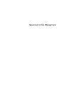
Figure 2.3: Ambiguity in a context-free grammar
variable must only allow using already-declared variables. This is a context de-
pendency. A grammar that contains a nonterminal whose use depends on the
context where it is used is called a context-sensitive grammar.
The syntax of most practical programming languages is therefore defined in
two parts (see Figure 2.2): as a context-free grammar supplemented with a set of
extra conditions imposed by the language. The context-free grammar is kept in-
stead of some more expressive notation because it is easy to read and understand.
It has an important locality property: a nonterminal symbol can be understood
by examining only the rules needed to define it; the (possibly much more numer-
ous) rules that use it can be ignored. The context-free grammar is corrected by
imposing a set of extra conditions, like the declare-before-use restriction on vari-
ables. Taking these conditions into account gives a context-sensitive grammar.
Ambiguity
Context-free grammars can be ambiguous, i.e., there can be several parse trees
that correspond to a given token sequence. For example, here is a simple grammar
for arithmetic expressions with addition and multiplication:
exp ::= int|expopexp
op ::= + | *
The expression 2*3+4 has two parse trees, depending on how the two occurrences
of exp are read. Figure 2.3 shows the two trees. In one tree, the first exp is 2
and the second exp is 3+4. In the other tree, they are 2*3 and 4, respectively.
Ambiguity is usually an undesirable property of a grammar since it makes
it unclear exactly what program is being written. In the expression 2*3+4,the

two parse trees give different results when evaluating the expression: one gives
14 (the result of computing 2*(3+4)) and the other gives 10 (the result of com-
puting (2*3)+4). Sometimes the grammar rules can be rewritten to remove the
ambiguity, but this can make the rules more complicated. A more convenient
approach is to add extra conditions. These conditions restrict the parser so that
only one parse tree is possible. We say that they disambiguate the grammar.
For expressions with binary operators such as the arithmetic expressions given
above, the usual approach is to add two conditions, precedence and associativity:
Copyright
c
 2001-3 by P. Van Roy and S. Haridi. All rights reserved.
2.1 Defining practical programming languages 37
• Precedence is a condition on an expression with different operators, like
2*3+4. Each operator is given a precedence level. Operators with high
precedences are put as deep in the parse tree as possible, i.e., as far away
from the root as possible. If * has higher precedence than +, then the parse
tree (2*3)+4 is chosen over the alternative 2*(3+4).If* is deeper in the
tree than +,thenwesaythat* binds tighter than +.
• Associativity is a condition on an expression with the same operator, like
2-3-4. In this case, precedence is not enough to disambiguate because all
operators have the same precedence. We have to choose between the trees
(2-3)-4 and 2-(3-4). Associativity determines whether the leftmost or
the rightmost operator binds tighter. If the associativity of - is left,then
the tree (2-3)-4 is chosen. If the associativity of - is right, then the other
tree 2-(3-4) is chosen.
Precedence and associativity are enough to disambiguate all expressions defined
with operators. Appendix C gives the precedence and associativity of all the
operators used in this book.
Syntax notation used in this book
In this chapter and the rest of the book, each new data type and language con-

struct is introduced together with a small syntax diagram that shows how it fits
in the whole language. The syntax diagram gives grammar rules for a simple
context-free grammar of tokens. The notation is carefully designed to satisfy two
basic principles:
• All grammar rules can stand on their own. No later information will ever
invalidate a grammar rule. That is, we never give an incorrect grammar
rule just to “simplify” the presentation.
• It is always clear by inspection when a grammar rule completely defines a
nonterminal symbol or when it gives only a partial definition. A partial
definition always ends in three dots “ ”.
All syntax diagrams used in the book are summarized in Appendix C. This
appendix also gives the lexical syntax of tokens, i.e., the syntax of tokens in
terms of characters. Here is an example of a syntax diagram with two grammar
rules that illustrates our notation:
statement ::=
skip |expression ´=´ expression|
expression ::= variable|int|
These rules give partial definitions of two nonterminals, statement and expression.
Thefirstrulesaysthatastatementcanbethekeyword
skip, or two expressions
separated by the equals symbol
=, or something else. The second rule says that
an expression can be a variable, an integer, or something else. To avoid confusion
Copyright
c
 2001-3 by P. Van Roy and S. Haridi. All rights reserved.
38 Declarative Computation Model
with the grammar rule’s own syntax, a symbol that occurs literally in the text
is always quoted with single quotes. For example, the equals symbol is shown as
´=´. Keywords are not quoted, since for them no confusion is possible. A choice

between different possibilities in the grammar rule is given by a vertical bar |.
Here is a second example to give the remaining notation:
statement ::=
if expression then statement
{
elseif expression then statement}
[
else statement ] end |
expression ::=
´[´ {expression}+ ´]´ |
label ::=
unit | true | false |variable|atom
The first rule defines the
if statement. There is an optional sequence of elseif
clauses, i.e., there can be any number of occurrences including zero. This is
denoted by the braces { }. This is followed by an optional
else clause, i.e., it
can occur zero or one times. This is denoted by the brackets [ ]. The second
rule defines the syntax of explicit lists. They must have at least one element, e.g.,
[5 6 7] is valid but []is not (note the space that separates the [ and the ]).
This is denoted by { }+. The third rule defines the syntax of record labels.
This is a complete definition. There are five possibilities and no more will ever
be given.
2.1.2 Language semantics
The semantics of a language defines what a program does when it executes.
Ideally, the semantics should be defined in a simple mathematical structure that
lets us reason about the program (including its correctness, execution time, and
memory use) without introducing any irrelevant details. Can we achieve this for a
practical language without making the semantics too complicated? The technique
we use, which we call the kernel language approach, gives an affirmative answer

to this question.
Modern programming languages have evolved through more than five decades
of experience in constructing programmed solutions to complex, real-world prob-
lems.
1
Modern programs can be quite complex, reaching sizes measured in mil-
lions of lines of code, written by large teams of human programmers over many
years. In our view, languages that scale to this level of complexity are successful
in part because they model some essential aspects of how to construct complex
programs. In this sense, these languages are not just arbitrary constructions of
the human mind. We would therefore like to understand them in a scientific way,
i.e., by explaining their behavior in terms of a simple underlying model. This is
the deep motivation behind the kernel language approach.
1
The figure of five decades is somewhat arbitrary. We measure it from the first working
stored-program computer, the Manchester Mark I. According to lab documents, it ran its first
program on June 21, 1948 [178].
Copyright
c
 2001-3 by P. Van Roy and S. Haridi. All rights reserved.
2.1 Defining practical programming languages 39
Practical language
Kernel language
Translation
proc {Sqr X Y}
fun {Sqr X} X*X end
B={Sqr {Sqr A}}
{’*’ X X Y}
end
end

{Sqr T B}
{Sqr A T}
local T in
- Has a formal semantics (e.g.,
an operational, axiomatic, or
denotational semantics)
-
intuitive concepts
Contains a minimal set of
Is easy for the programmer
to understand and reason in
-
for the programmer
Provides useful abstractions-
Can be extended with
linguistic abstractions
-
Figure 2.4: The kernel language approach to semantics
The kernel language approach
This book uses the kernel language approach to define the semantics of program-
ming languages. In this approach, all language constructs are defined in terms
of translations into a core language known as the kernel language. The kernel
language approach consists of two parts (see Figure 2.4):
• First, define a very simple language, called the kernel language.Thislan-
guage should be easy to reason in and be faithful to the space and time
efficiency of the implementation. The kernel language and the data struc-
tures it manipulates together form the kernel computation model.
• Second, define a translation scheme from the full programming language
to the kernel language. Each grammatical construct in the full language is
translated into the kernel language. The translation should be as simple as

possible. There are two kinds of translation, namely linguistic abstraction
and syntactic sugar. Both are explained below.
The kernel language approach is used throughout the book. Each computation
model has its kernel language, which builds on its predecessor by adding one new
concept. The first kernel language, which is presented in this chapter, is called
the declarative kernel language. Many other kernel languages are presented later
on in the book.
Formal semantics
The kernel language approach lets us define the semantics of the kernel language in
any way we want. There are four widely-used approaches to language semantics:
Copyright
c
 2001-3 by P. Van Roy and S. Haridi. All rights reserved.
40 Declarative Computation Model
• An operational semantics shows how a statement executes in terms of an
abstract machine. This approach always works well, since at the end of the
day all languages execute on a computer.
• An axiomatic semantics defines a statement’s semantics as the relation be-
tween the input state (the situation before executing the statement) and
the output state (the situation after executing the statement). This relation
is given as a logical assertion. This is a good way to reason about state-
ment sequences, since the output assertion of each statement is the input
assertion of the next. It therefore works well with stateful models, since a
state is a sequence of values. Section 6.6 gives an axiomatic semantics of
Chapter 6’s stateful model.
• A denotational semantics defines a statement as a function over an ab-
stract domain. This works well for declarative models, but can be applied
to other models as well. It gets complicated when applied to concurrent
languages. Sections 2.7.1 and 4.9.2 explain functional programming, which
is particularly close to denotational semantics.

• A logical semantics defines a statement as a model of a logical theory. This
works well for declarative and relational computation models, but is hard
to apply to other models. Section 9.3 gives a logical semantics of the declar-
ative and relational computation models.
Much of the theory underlying these different semantics is of interest primarily to
mathematicians, not to programmers. It is outside the scope of the book to give
this theory. The principal formal semantics we give in this book is an operational
semantics. We define it for each computation model. It is detailed enough to
be useful for reasoning about correctness and complexity yet abstract enough to
avoid irrelevant clutter. Chapter 13 collects all these operational semantics into
a single formalism with a compact and readable notation.
Throughout the book, we give an informal semantics for every new language
construct and we often reason informally about programs. These informal pre-
sentations are always based on the operational semantics.
Linguistic abstraction
Both programming languages and natural languages can evolve to meet their
needs. When using a programming language, at some point we may feel the need
to extend the language, i.e., to add a new linguistic construct. For example, the
declarative model of this chapter has no looping constructs. Section 3.6.3 defines
a
for construct to express certain kinds of loops that are useful for writing
declarative programs. The new construct is both an abstraction and an addition
to the language syntax. We therefore call it a linguistic abstraction.Apractical
programming language consists of a set of linguistic abstractions.
Copyright
c
 2001-3 by P. Van Roy and S. Haridi. All rights reserved.
2.1 Defining practical programming languages 41
There are two phases to defining a linguistic abstraction. First, define a new
grammatical construct. Second, define its translation into the kernel language.

The kernel language is not changed. This book gives many examples of useful
linguistic abstractions, e.g., functions (
fun), loops (for), lazy functions (fun
lazy
), classes (class), reentrant locks (lock), and others.
2
Some of these are
part of the Mozart system. The others can be added to Mozart with the gump
parser-generator tool [104]. Using this tool is beyond the scope of this book.
A simple example of a linguistic abstraction is the function syntax, which
uses the keyword
fun. This is explained in Section 2.5.2. We have already
programmed with functions in Chapter 1. But the declarative kernel language
of this chapter only has procedure syntax. Procedure syntax is chosen for the
kernel since all arguments are explicit and there can be multiple outputs. There
are other, deeper reasons for choosing procedure syntax which are explained later
in this chapter. Because function syntax is so useful, though, we add it as a
linguistic abstraction.
We define a syntax for both function definitions and function calls, and a
translation into procedure definitions and procedure calls. The translation lets
us answer all questions about function calls. For example, what does
{F1 {F2
X} {F3 Y}}
mean exactly (nested function calls)? Is the order of these function
calls defined? If so, what is the order? There are many possibilities. Some
languages leave the order of argument evaluation unspecified, but assume that a
function’s arguments are evaluated before the function. Other languages assume
that an argument is evaluated when and if its result is needed, not before. So even
as simple a thing as nested function calls does not necessarily have an obvious
semantics. The translation makes it clear what the semantics is.

Linguistic abstractions are useful for more than just increasing the expressive-
ness of a program. They can also improve other properties such as correctness,
security, and efficiency. By hiding the abstraction’s implementation from the pro-
grammer, the linguistic support makes it impossible to use the abstraction in the
wrong way. The compiler can use this information to give more efficient code.
Syntactic sugar
It is often convenient to provide a short-cut notation for frequently-occurring
idioms. This notation is part of the language syntax and is defined by grammar
rules. This notation is called syntactic sugar. Syntactic sugar is analogous to
linguistic abstraction in that its meaning is defined precisely by translating it
into the full language. But it should not be confused with linguistic abstraction:
it does not provide a new abstraction, but just reduces program size and improves
program readability.
We give an example of syntactic sugar that is based on the
local statement.
2
Logic gates (gate) for circuit descriptions, mailboxes (receive) for message-passing
concurrency, and currying and list comprehensions as in modern functional languages, cf.,
Haskell.
Copyright
c
 2001-3 by P. Van Roy and S. Haridi. All rights reserved.
42 Declarative Computation Model
Programming language
Mathematical study
of programming
Foundational calculusKernel language Abstract machine
Efficient execution
on a real machine
Aid the programmer

in reasoning and
understanding
Translations
Figure 2.5: Translation approaches to language semantics
Local variables can always be defined by using the statement
local X in
end
. When this statement is used inside another, it is convenient to have syntactic
sugar that lets us leave out the keywords
local and end. Instead of:
if N==1 then [1]
else
local L in

end
end
we can write:
if N==1 then [1]
else L in

end
which is both shorter and more readable than the full notation. Other examples
of syntactic sugar are given in Section 2.5.1.
Language design
Linguistic abstractions are a basic tool for language design. Any abstraction that
we define has three phases in its lifecycle. When first we define it, it has no lin-
guistic support, i.e., there is no syntax in the language designed to make it easy
to use. If at some point, we suspect that it is especially basic and useful, we can
decide to give it linguistic support. It then becomes a linguistic abstraction. This
is an exploratory phase, i.e., there is no commitment that the linguistic abstrac-

tion will become part of the language. If the linguistic abstraction is successful,
i.e., it simplifies programs and is useful to programmers, then it becomes part of
the language.
Copyright
c
 2001-3 by P. Van Roy and S. Haridi. All rights reserved.
2.1 Defining practical programming languages 43
Other translation approaches
The kernel language approach is an example of a translation approach to seman-
tics, i.e., it is based on a translation from one language to another. Figure 2.5
shows the three ways that the translation approach has been used for defining
programming languages:
• The kernel language approach, used throughout the book, is intended for the
programmer. Its concepts correspond directly to programming concepts.
• The foundational approach is intended for the mathematician. Examples
are the Turing machine, the λ calculus (underlying functional program-
ming), first-order logic (underlying logic programming), and the π calculus
(to model concurrency). Because these calculi are intended for formal math-
ematical study, they have as few elements as possible.
• The machine approach is intended for the implementor. Programs are trans-
lated into an idealized machine, which is traditionally called an abstract
machine or a virtual machine.
3
It is relatively easy to translate idealized
machine code into real machine code.
Because we focus on practical programming techniques, this book uses only the
kernel language approach.
The interpreter approach
An alternative to the translation approach is the interpreter approach. The lan-
guage semantics is defined by giving an interpreter for the language. New lan-

guage features are defined by extending the interpreter. An interpreter is a pro-
gram written in language L
1
that accepts programs written in another language
L
2
and executes them. This approach is used by Abelson & Sussman [2]. In their
case, the interpreter is metacircular, i.e., L
1
and L
2
are the same language L.
Adding new language features, e.g., for concurrency and lazy evaluation, gives a
new language L

which is implemented by extending the interpreter for L.
The interpreter approach has the advantage that it shows a self-contained
implementation of the linguistic abstractions. We do not use the interpreter
approach in this book because it does not in general preserve the execution-time
complexity of programs (the number of operations needed as a function of input
size). A second difficulty is that the basic concepts interact with each other in
the interpreter, which makes them harder to understand.
3
Strictly speaking, a virtual machine is a software emulation of a real machine, running on
the real machine, that is almost as efficient as the real machine. It achieves this efficiency by
executing most virtual instructions directly as real instructions. The concept was pioneered by
IBM in the early 1960’s in the VM operating system. Because of the success of Java, which
uses the term “virtual machine”, modern usage tends to blur the distinction between abstract
and virtual machines.
Copyright

c
 2001-3 by P. Van Roy and S. Haridi. All rights reserved.
44 Declarative Computation Model
unbound
unbound
unbound
x
x
x
3
2
1
Figure 2.6: A single-assignment store with three unbound variables
unbound
x
x
x
3
2
1
314
nil123
Figure 2.7: Two of the variables are bound to values
2.2 The single-assignment store
We introduce the declarative model by first explaining its data structures. The
model uses a single-assignment store, which is a set of variables that are initially
unbound and that can be bound to one value. Figure 2.6 shows a store with three
unbound variables x
1
, x

2
,andx
3
. Wecanwritethisstoreas{x
1
,x
2
,x
3
}.For
now, let us assume we can use integers, lists, and records as values. Figure 2.7
shows the store where x
1
is bound to the integer 314 and x
2
is bound to the list
[1 2 3]. We write this as {x
1
= 314,x
2
= [123],x
3
}.
2.2.1 Declarative variables
Variables in the single-assignment store are called declarative variables. We use
this term whenever there is a possible confusion with other kinds of variables.
Later on in the book, we will also call these variables dataflow variables because
of their role in dataflow execution.
Once bound, a declarative variable stays bound throughout the computation
and is indistinguishable from its value. What this means is that it can be used

in calculations as if it were the value. Doing the operation x + y is the same as
doing 11 + 22, if the store is {x =11,y =22}.
2.2.2 Value store
A store where all variables are bound to values is called a value store.Another
way to say this is that a value store is a persistent mapping from variables to
Copyright
c
 2001-3 by P. Van Roy and S. Haridi. All rights reserved.
2.2 The single-assignment store 45
"George" 25
x
x
x
3
2
1
314
nil123
person
name age
Figure 2.8: A value store: all variables are bound to values
values. A value is a mathematical constant. For example, the integer 314 is
a value. Values can also be compound entities. For example, the list
[1 2
3]
and the record person(name:"George" age:25) are values. Figure 2.8
shows a value store where x
1
is bound to the integer 314, x
2

is bound to the
list
[123],andx
3
is bound to the record person(name:"George" age:25).
Functional languages such as Standard ML, Haskell, and Scheme get by with a
value store since they compute functions on values. (Object-oriented languages
such as Smalltalk, C++, and Java need a cell store, which consists of cells whose
content can be modified.)
At this point, a reader with some programming experience may wonder why
we are introducing a single-assignment store, when other languages get by with
a value store or a cell store. There are many reasons. The first reason is that
we want to compute with partial values. For example, a procedure can return an
output by binding an unbound variable argument. The second reason is declara-
tive concurrency, which is the subject of Chapter 4. It is possible because of the
single-assignment store. The third reason is that it is essential when we extend the
model to deal with relational (logic) programming and constraint programming.
Other reasons having to do with efficiency (e.g., tail recursion and difference lists)
will become clear in the next chapter.
2.2.3 Value creation
The basic operation on a store is binding a variable to a newly-created value. We
will write this as x
i
=value.Herex
i
refers directly to a variable in the store (and
is not the variable’s textual name in a program!) and value refers to a value, e.g.,
314 or
[1 2 3]. For example, Figure 2.7 shows the store of Figure 2.6 after the
two bindings:

x
1
= 314
x
2
= [1 2 3]
Copyright
c
 2001-3 by P. Van Roy and S. Haridi. All rights reserved.
46 Declarative Computation Model
x
1
unbound"X"
Inside the storeIn statement
Figure 2.9: A variable identifier referring to an unbound variable
nil123
x
1
"X"
Inside the store
Figure 2.10: A variable identifier referring to a bound variable
The single-assignment operation x
i
=value constructs value in the store and then
binds the variable x
i
to this value. If the variable is already bound, the operation
will test whether the two values are compatible. If they are not compatible, an
error is signaled (using the exception-handling mechanism, see Section 2.6).
2.2.4 Variable identifiers

So far, we have looked at a store that contains variables and values, i.e., store
entities, with which calculations can be done. It would be nice if we could refer
to a store entity from outside the store. This is the role of variable identifiers.
A variable identifier is a textual name that refers to a store entity from outside
the store. The mapping from variable identifiers to store entities is called an
environment.
The variable names in program source code are in fact variable identifiers.
For example, Figure 2.9 has an identifier “
X” (the capital letter X) that refers to
the store variable x
1
. This corresponds to the environment {X → x
1
}.Totalk
about any identifier, we will use the notation x. The environment {x→x
1
}
is the same as before, if x represents
X. As we will see later, variable identifiers
and their corresponding store entities are added to the environment by the
local
and declare statements.
Copyright
c
 2001-3 by P. Van Roy and S. Haridi. All rights reserved.
2.2 The single-assignment store 47
x
1
nil123"X"
Inside the store

Figure 2.11: A variable identifier referring to a value
x
1
x
2
person
unbound"George"
name age
"X"
"Y"
Inside the store
Figure 2.12: A partial value
2.2.5 Value creation with identifiers
Once bound, a variable is indistinguishable from its value. Figure 2.10 shows what
happens when x
1
is bound to [123]in Figure 2.9. With the variable identifier
X, we can write the binding as X=[1 2 3]. This is the text a programmer would
write to express the binding. We can also use the notation x
=[1 2 3] if we
want to be able to talk about any identifier. To make this notation legal in a
program, x has to be replaced by an identifier.
The equality sign “
=” refers to the bind operation. After the bind completes,
the identifier “
X” still refers to x
1
, which is now bound to [1 2 3].Thisis
indistinguishable from Figure 2.11, where
X refers directly to [123]. Following

the links of bound variables to get the value is called dereferencing. It is invisible
to the programmer.
2.2.6 Partial values
A partial value is a data structure that may contain unbound variables. Fig-
ure 2.12 shows the record
person(name:"George" age:x
2
), referred to by the
identifier
X. This is a partial value because it contains the unbound variable x
2
.
The identifier
Y refers to x
2
. Figure 2.13 shows the situation after x
2
is bound
to 25 (through the bind operation
Y=25). Now x
1
is a partial value with no
unbound variables, which we call a complete value. A declarative variable can
Copyright
c
 2001-3 by P. Van Roy and S. Haridi. All rights reserved.
48 Declarative Computation Model
x
1
x

2
person
25"George"
name age
"X"
"Y"
Inside the store
Figure 2.13: A partial value with no unbound variables, i.e., a complete value
x
1
"X"
"Y" x
2
Inside the store
Figure 2.14: Two variables bound together
be bound to several partial values, as long as they are compatible with each
other. We say a set of partial values is compatible if the unbound variables in
them can be bound in such a way as to make them all equal. For example,
person(age:25) and person(age:x) are compatible (because x can be bound
to 25), but
person(age:25) and person(age:26) are not.
2.2.7 Variable-variable binding
Variables can be bound to variables. For example, consider two unbound variables
x
1
and x
2
referred to by the identifiers X and Y. After doing the bind X=Y,weget
the situation in Figure 2.14. The two variables x
1

and x
2
are equal to each other.
The figure shows this by letting each variable refer to the other. We say that
{x
1
, x
2
} form an equivalence set.
4
We also write this as x
1
= x
2
.Threevariables
that are bound together are written as x
1
= x
2
= x
3
or {x
1
, x
2
, x
3
}.Drawnin
a figure, these variables would form a circular chain. Whenever one variable in
an equivalence set is bound, then all variables see the binding. Figure 2.15 shows

the result of doing
X=[1 2 3].
4
From a formal viewpoint, the two variables form an equivalence class with respect to equal-
ity.
Copyright
c
 2001-3 by P. Van Roy and S. Haridi. All rights reserved.
2.2 The single-assignment store 49
x
1
1 2 3 nil
Inside the store
"X"
"Y" x
2
Figure 2.15: The store after binding one of the variables
2.2.8 Dataflow variables
In the declarative model, creating a variable and binding it are done separately.
What happens if we try to use the variable before it is bound? We call this a
variable use error. Some languages create and bind variables in one step, so that
use errors cannot occur. This is the case for functional programming languages.
Other languages allow creating and binding to be separate. Then we have the
following possibilities when there is a use error:
1. Execution continues and no error message is given. The variable’s content
is undefined, i.e. it is “garbage”: whatever is found in memory. This is
what C++ does.
2. Execution continues and no error message is given. The variable is initial-
ized to a default value when it is declared, e.g., to 0 for an integer. This is
what Java does.

3. Execution stops with an error message (or an exception is raised). This is
what Prolog does for arithmetic operations.
4. Execution waits until the variable is bound and then continues.
These cases are listed in increasing order of niceness. The first case is very bad,
since different executions of the same program can give different results. What’s
more, since the existence of the error is not signaled, the programmer is not even
aware when this happens. The second is somewhat better. If the program has a
use error, then at least it will always give the same result, even if it is a wrong
one. Again the programmer is not made aware of the error’s existence.
The third and fourth cases are reasonable in certain situations. In the third,
a program with a use error will signal this fact, instead of silently continuing.
This is reasonable in a sequential system, since there really is an error. It is
unreasonable in a concurrent system, since the result becomes nondeterministic:
depending on the timing, sometimes an error is signaled and sometimes not. In
the fourth, the program will wait until the variable is bound, and then continue.
This is unreasonable in a sequential system, since the program will wait forever.
Copyright
c
 2001-3 by P. Van Roy and S. Haridi. All rights reserved.
50 Declarative Computation Model
s ::=
skip Empty statement
|s
1
s
2
Statement sequence
|
local x in s end Variable creation
|x

1
=x
2
Variable-variable binding
|x=v Value creation
|
if x then s
1
else s
2
end Conditional
|
case x of pattern then s
1
else s
2
end Pattern matching
|
{xy
1
y
n
} Procedure application
Table 2.1: The declarative kernel language
It is reasonable in a concurrent system, where it could be part of normal operation
that some other thread binds the variable.
5
The computation models of this book
use the fourth case.
Declarative variables that cause the program to wait until they are bound are

called dataflow variables. The declarative model uses dataflow variables because
they are tremendously useful in concurrent programming, i.e., for programs with
activities that run independently. If we do two concurrent operations, say
A=23
and B=A+1, then with the fourth solution this will always run correctly and give
the answer
B=24. It doesn’t matter whether A=23 is tried first or whether B=A+1
is tried first. With the other solutions, there is no guarantee of this. This property
of order-independence makes possible the declarative concurrency of Chapter 4.
It is at the heart of why dataflow variables are a good idea.
2.3 Kernel language
The declarative model defines a simple kernel language. All programs in the
model can be expressed in this language. We first define the kernel language
syntax and semantics. Then we explain how to build a full language on top of
the kernel language.
2.3.1 Syntax
The kernel syntax is given in Tables 2.1 and 2.2. It is carefully designed to be a
subset of the full language syntax, i.e., all statements in the kernel language are
valid statements in the full language.
5
Still, during development, a good debugger should capture undesirable suspensions if there
are no other running threads.
Copyright
c
 2001-3 by P. Van Roy and S. Haridi. All rights reserved.
2.3 Kernel language 51
v ::= number|record|procedure
number ::= int|float
record, pattern ::= literal
|literal(feature

1
: x
1
feature
n
: x
n
)
procedure ::=
proc {$x
1
x
n
} s end
literal ::= atom|bool
feature ::= atom|bool|int
bool ::=
true | false
Table 2.2: Value expressions in the declarative kernel language
Statement syntax
Table 2.1 defines the syntax of s, which denotes a statement. There are eight
statements in all, which we will explain later.
Value syntax
Table 2.2 defines the syntax of v, which denotes a value. There are three kinds
of value expressions, denoting numbers, records, and procedures. For records and
patterns, the arguments x
1
, , x
n
must all be distinct identifiers. This ensures

that all variable-variable bindings are written as explicit kernel operations.
Variable identifier syntax
Table 2.1 uses the nonterminals x and y to denote a variable identifier. We
will also use z to denote identifiers. There are two ways to write a variable
identifier:
• An uppercase letter followed by zero or more alphanumeric characters (let-
ters or digits or underscores), for example
X, X1,orThisIsALongVariable_IsntIt.
• Any sequence of printable characters enclosed within
‘ (back-quote) char-
acters, e.g.,
`this is a 25$\variable!`.
A precise definition of identifier syntax is given in Appendix C. All newly-declared
variables are unbound before any statement is executed. All variable identifiers
must be declared explicitly.
2.3.2 Values and types
A type or data type is a set of values together with a set of operations on those
values. A value is “of a type” if it is in the type’s set. The declarative model
is typed in the sense that it has a well-defined set of types, called basic types.
For example, programs can calculate with integers or with records, which are all
Copyright
c
 2001-3 by P. Van Roy and S. Haridi. All rights reserved.
52 Declarative Computation Model
of integer type or record type, respectively. Any attempt to use an operation
with values of the wrong type is detected by the system and will raise an error
condition (see Section 2.6). The model imposes no other restrictions on the use
of types.
Because all uses of types are checked, it is not possible for a program to behave
outside of the model, e.g., to crash because of undefined operations on its internal

data structures. It is still possible for a program to raise an error condition, for
example by dividing by zero. In the declarative model, a program that raises
an error condition will terminate immediately. There is nothing in the model to
handle errors. In Section 2.6 we extend the declarative model with a new concept,
exceptions, to handle errors. In the extended model, type errors can be handled
within the model.
In addition to basic types, programs can define their own types, which are
called abstract data types, ADT for short. Chapter 3 and later chapters show
how to define ADTs.
Basic types
The basic types of the declarative model are numbers (integers and floats), records
(including atoms, booleans, tuples, lists, and strings), and procedures. Table 2.2
gives their syntax. The nonterminal v denotes a partially constructed value.
Later in the book we will see other basic types, including chunks, functors, cells,
dictionaries, arrays, ports, classes, and objects. Some of these are explained in
Appendix B.
Dynamic typing
There are two basic approaches to typing, namely dynamic and static typing. In
static typing, all variable types are known at compile time. In dynamic typing,
the variable type is known only when the variable is bound. The declarative
model is dynamically typed. The compiler tries to verify that all operations use
values of the correct type. But because of dynamic typing, some type checks are
necessarily left for run time.
The type hierarchy
The basic types of the declarative model can be classified into a hierarchy. Fig-
ure 2.16 shows this hierarchy, where each node denotes a type. The hierarchy
is ordered by set inclusion, i.e., all values of a node’s type are also values of the
parent node’s type. For example, all tuples are records and all lists are tuples.
This implies that all operations of a type are also legal for a subtype, e.g., all
list operations work also for strings. Later on in the book we will extend this

hierarchy. For example, literals can be either atoms (explained below) or another
kind of constant called names (see Section 3.7.5). The parts where the hierarchy
is incomplete are given as “ ”.
Copyright
c
 2001-3 by P. Van Roy and S. Haridi. All rights reserved.
2.3 Kernel language 53
Literal

Int Float
Number Record
Tuple
Value
Procedure
AtomBool
True False
Char List
String

Figure 2.16: The type hierarchy of the declarative model
2.3.3 Basic types
We give some examples of the basic types and how to write them. See Appendix B
for more complete information.
• Numbers. Numbers are either integers or floating point numbers. Exam-
ples of integers are
314, 0,and˜10 (minus 10). Note that the minus sign
is written with a tilde “
˜”. Examples of floating point numbers are 1.0,
3.4, 2.0e2,and˜2.0E˜2.
• Atoms. An atom is a kind of symbolic constant that can be used as a

single element in calculations. There are several different ways to write
atoms. An atom can be written as a sequence of characters starting with
a lowercase letter followed by any number of alphanumeric characters. An
atom can also be written as any sequence of printable characters enclosed
in single quotes. Examples of atoms are
a_person, donkeyKong3,and
´#### hello ####´.
• Booleans. A boolean is either the symbol
true or the symbol false.
• Records. A record is a compound data structure. It consists of a label
followed by a set of pairs of features and variable identifiers. Features can
be atoms, integers, or booleans. Examples of records are
person(age:X1
name:X2)
(with features age and name), person(1:X1 2:X2), ´|´(1:H
2:T)
, ´#´(1:H 2:T), nil,andperson. An atom is a record with no
features.
• Tuples. A tuple is a record whose features are consecutive integers starting
from 1. The features do not have to be written in this case. Examples of
Copyright
c
 2001-3 by P. Van Roy and S. Haridi. All rights reserved.