Introduction to GPS The Global Positioning System - Part 2 docx
Bạn đang xem bản rút gọn của tài liệu. Xem và tải ngay bản đầy đủ của tài liệu tại đây (173.96 KB, 13 trang )
2
GPS Details
Positioning, or finding the users location, with GPS requires some under-
standing of the GPS signal structure and how the measurements can be
made. Likewise, as the GPS signal is received through a GPS receiver,
understanding the capabilities and limitations of the various types of GPS
receivers is essential. Furthermore, the GPS measurements, like all meas-
urable quantities, contain errors and biases, which can be removed or
reduced by combining the various GPS observables. This chapter discusses
these issues in detail.
2.1 GPS signal structure
As mentioned in Chapter 1, each GPS satellite transmits a microwave radio
signal composed of two carrier frequencies (or sine waves) modulated by
two digital codes and a navigation message (see Figure 2.1). The two carrier
frequencies are generated at 1,575.42 MHz (referred to as the L1 carrier)
and 1,227.60 MHz (referred to as the L2 carrier). The corresponding car-
rier wavelengths are approximately 19 cm and 24.4 cm, respectively, which
result from the relation between the carrier frequency and the speed of
13
TEAMFLY
Team-Fly
®
light in space [1, 2]. The availability of the two carrier frequencies allows
for correcting a major GPS error, known as the ionospheric delay (see
Chapter 3 for details). All of the GPS satellites transmit the same L1 and L2
carrier frequencies. The code modulation, however, is different for each
satellite, which significantly minimizes the signal interference.
The two GPS codes are called coarse acquisition (or C/A-code) and
precision (or P-code). Each code consists of a stream of binary digits, zeros
and ones, known as bits or chips. The codes are commonly known as PRN
codes because they look like random signals (i.e., they are noise-like sig-
nals). But in reality, the codes are generated using a mathematical algo-
rithm. Presently, the C/A-code is modulated onto the L1 carrier only,
while the P-code is modulated onto both the L1 and the L2 carriers. This
modulation is called biphase modulation, because the carrier phase is
shifted by 180° when the code value changes from zero to one or from one
to zero [3].
The C/A-code is a stream of 1,023 binary digits (i.e., 1,023 zeros and
ones) that repeats itself every millisecond. This means that the chipping
rate of the C/A-code is 1.023 Mbps. In other words, the duration of one bit
is approximately 1 ms, or equivalently 300m [4]. Each satellite is assigned a
unique C/A-code, which enables the GPS receivers to identify which satel-
lite is transmitting a particular code. The C/A-code range measurement is
relatively less precise compared with that of the P-code. It is, however, less
complex and is available to all users.
The P-code is a very long sequence of binary digits that repeats itself
after 266 days [1]. It is also 10 times faster than the C/A-code (i.e., its rate is
10.23 Mbps). Multiplying the time it takes the P-code to repeat itself, 266
days, by its rate, 10.23 Mbps, tells us that the P-code is a stream of about
2.35 × 10
14
chips! The 266-day-long code is divided into 38 segments; each
is 1 week long. Of these, 32 segments are assigned to the various GPS satel-
lites. That is, each satellite transmits a unique 1-week segment of the
P-code, which is initialized every Saturday/Sunday midnight crossing. The
remaining six segments are reserved for other uses. It is worth mentioning
that a GPS satellite is usually identified by its unique 1-week segment of the
P-code. For example, a GPS satellite with an ID of PRN 20 refers to a GPS
satellite that is assigned the twentieth-week segment of the PRN P-code.
The P-code is designed primarily for military purposes. It was available to
all users until January 31, 1994 [1]. At that time, the P-code was encrypted
by adding to it an unknown W-code. The resulting encrypted code is called
14 Introduction to GPS
the Y-code, which has the same chipping rate as the P-code. This encryp-
tion is known as the antispoofing (AS).
The GPS navigation message is a data stream added to both the L1 and
the L2 carriers as binary biphase modulation at a low rate of 50 kbps. It
consists of 25 frames of 1,500 bits each, or 37,500 bits in total. This means
that the transmission of the complete navigation message takes 750 sec-
onds, or 12.5 minutes. The navigation message contains, along with other
information, the coordinates of the GPS satellites as a function of time, the
satellite health status, the satellite clock correction, the satellite almanac,
and atmospheric data. Each satellite transmits its own navigation message
with information on the other satellites, such as the approximate location
and health status [1].
2.2 GPS modernization
The current GPS signal structure was designed in the early 1970s, some 30
years ago [5]. In the next 30 years, GPS constellation is expected to have a
combination of Block IIR satellites, currently being launched, and Block
IIF and possibly Block III satellites. To meet the future requirements, the
GPS decision makers have studied several options to adequately modify the
signal structure and system architecture of the future GPS constellation.
The modernization program aims, among other things, to provide signal
redundancy and improve positioning accuracy, signal availability, and sys-
tem integrity.
The modernization program will include the addition of a civil code
(C/A-code) on the L2 frequency and two new military codes (M-codes) on
both the L1 and the L2 frequencies [5]. These codes will be added to the last
12 Block IIR satellites, which will be launched at the beginning of 2003.
The availability of two civil codes (i.e., C/A-code on both L1 and L2
GPS Details 15
l
0
1
000011101001101000111100110
(
a
)(
b
)
Figure 2.1 (a) A sinusoidal wave; and (b) a digital code.
frequencies) allows a user with a stand-alone GPS receiver to correct for the
effect of the ionosphere (the upper layer of the atmosphere), which is a
major error source (see Chapter 3 for details). With the termination of
selective availability, it is expected that once a sufficient number of satel-
lites with the new capabilities is available, the autonomous GPS horizontal
accuracy will be about 8.5m (95% of the time) or better [5].
The addition of the C/A-code to L2, although it improves the autono-
mous GPS accuracy, was found to be insufficient for use in the civil avia-
tion safety-of-life applications. This is mainly because of the potential
interference from the ground radars that operate near the GPS L2 band. As
such, to satisfy aviation user requirements, a third civil signal at 1,176.45
MHz (called L5) will be added to the first 12 Block IIF satellites along with
the C/A-code on L2 and the M-code on L1 and L2, as part of the moderni-
zation program [5]. This third frequency will be robust and will have a
higher power level. In addition, this new L5 signal will have wide broadcast
bandwidth (a minimum of 20 MHz) and a higher chipping rate (10.23
MHz), which provide higher accuracy under noisy and multipath condi-
tions. The new code will be longer than the current C/A-code, which
reduces the system self-interference through the improvement of the auto-
and cross-correlation properties. Finally, the broadcast navigation message
of the new signal, although containing more or less the same data as the L1
and L2 channels, will have an entirely different, more efficient, structure.
The first Block IIF satellite is scheduled to be launched in 2005 or shortly
after that date. The addition of these capabilities will dramatically improve
the autonomous GPS positioning accuracy. As well, the real-time kine-
matic (RTK) users, who require centimeter-level accuracy in real time, will
be able to resolve the initial integer ambiguity parameters instantaneously.
More about RTK positioning is given in Chapter 5.
The modernization of GPS will also include the studies for the next
generation Block III satellites, which will carry GPS into 2030. Finally, the
GPS ground control facilities will also be upgraded as a part of the GPS
modernization program. With this upgrade, the expected standalone GPS
horizontal accuracy will be 6m (95% of the time) or better [5].
2.3 Types of GPS receivers
In 1980, only one commercial GPS receiver was available on the market, at
a price of several hundred thousand U.S. dollars [6]. This, however, has
16 Introduction to GPS
changed considerably as more than 500 different GPS receivers are avail-
able in todays market (see, for example, the January 2001 issue of GPS
World magazine). The current receiver price varies from about $100 for the
simple handheld units to about $15,000 for the sophisticated geodetic
quality units. The price will continue to decline in the future as the receiver
technology becomes more advanced. A GPS receiver requires an antenna
attached to it, either internally or externally. The antenna receives the
incoming satellite signal and then converts its energy into an electric cur-
rent, which can be handled by the GPS receiver [6, 7].
Commercial GPS receivers may be divided into four types, according
to their receiving capabilities. These are: single-frequency code receivers,
single-frequency carrier-smoothed code receivers, single-frequency code
and carrier receivers, and dual-frequency receivers. Single-frequency
receivers access the L1 frequency only, while dual-frequency receivers
access both the L1 and the L2 frequencies. Figure 2.2 shows examples of
various types of GPS receivers. GPS receivers can also be categorized
according to their number of tracking channels, which varies from 1 to 12
channels. A good GPS receiver would be multichannel, with each channel
dedicated to continuously tracking a particular satellite. Presently, most
GPS receivers have 9 to 12 independent (or parallel) channels. Features
such as cost, ease of use, power consumption, size and weight, internal
and/or external data-storage capabilities, interfacing capabilities, and mul-
tipath mitigation (i.e., type of correlator) are to be considered when select-
ing a GPS receiver.
The first receiver type, the single-frequency code receiver, measures
the pseudoranges with the C/A-code only. No other measurements are
available. It is the least expensive and the least accurate receiver type, and is
mostly used for recreation purposes. The second receiver type, the single-
frequency carrier-smoothed code receiver, also measures the pseudoranges
with the C/A-code only. However, with this receiver type, the higher-
resolution carrier frequency is used internally to improve the resolution
of the code pseudorange, which results in high-precision pseudorange
measurements. Single-frequency code and carrier receivers output the raw
C/A-code pseudoranges, the L1 carrier-phase measurements, and the navi-
gation message. In addition, this receiver type is capable of performing the
functions of the other receiver types discussed above.
Dual-frequency receivers are the most sophisticated and most expen-
sive receiver type. Before the activation of AS, dual-frequency receivers
GPS Details 17
were capable of outputting all of the GPS signal components (i.e., L1 and
L2 carriers, C/A-code, P-code on both L1 and L2, and the navigation mes-
sage). However, after the AS activation, the P-code was encrypted to
Y-code. This means that the receiver cannot output either the P-code or
the L2 carrier using the traditional signal-recovering technique. To over-
come this problem, GPS receiver manufacturers invented a number of
techniques that do not require information of the Y-code. At the present
time, most receivers use two techniques known as the Z-tracking and the
cross-correlation techniques. Both techniques recover the full L2 carrier,
but at a degraded signal strength. The amount of signal strength degrad-
ation is higher in the cross-correlation techniques compared with the
Z-tracking technique.
2.4 Time systems
Time plays a very important role in positioning with GPS. As explained in
Chapter 1, the GPS signal is controlled by accurate timing devices, the
atomic satellite clocks [8]. In addition, measuring the ranges (distances)
from the receiver to the satellites is based on both the receiver and the
18 Introduction to GPS
Magellan handheld
GPS receiver
Ashtech ZX geodetic quality
GPS receiver
Figure 2.2 Examples of GPS receivers. (Courtesy of Magellan Corporation.)
satellite clocks. GPS is also a timing system, that is, it can be used for time
synchronization.
A number of time systems are used worldwide for various purposes
[1]. Of these, the Coordinated Universal Time (UTC) and the GPS Time
are the most important to GPS users. UTC is an atomic time scale based on
the International Atomic Time (TAI). TAI is a uniform time scale, which is
computed based on independent time scales generated by atomic clocks
located at various timing laboratories throughout the world. In surveying
and navigation, however, a time system with relation to the rotation of the
Earth, not the atomic time, is desired. This is achieved by occasionally
adjusting the UTC time scale by 1-second increments, known as leap sec-
onds, to keep it within 0.9 second of another time scale called the Universal
Time 1 (UT1) [8, 9], where UT1 is a universal time that gives a measure of
the rotation of the Earth. Leap seconds are introduced occasionally, on
either June 30 or December 31. As of July 2001, the last leap second was
introduced on January 1, 1999, which made the difference between TAI
and UTC time scales to be exactly 32 seconds (TAI is ahead of UTC). Infor-
mation about the leap seconds can be found at the U.S. Naval Observatory
Web site, .
GPS Time is the time scale used for referencing, or time tagging, the
GPS signals. It is computed based on the time scales generated by the
atomic clocks at the monitor stations and onboard GPS satellites. There are
no leap seconds introduced into GPS Time, which means that GPS Time is
a continuous time scale. GPS Time scale was set equal to that of the UTC on
January 6, 1980 [8]. However, due to the leap seconds introduced into the
UTC time scale, GPS Time moved ahead of the UTC by 13 seconds on
January 1, 1999. The difference between GPS and UTC time scales is given
in the GPS navigation message. It is worth mentioning that, as shown in
Chapter 3, both GPS satellite and receiver clocks are offset from the GPS
Time, as a result of satellite and receiver clock errors.
2.5 Pseudorange measurements
The pseudorange is a measure of the range, or distance, between the GPS
receiver and the GPS satellite (more precisely, it is the distance between the
GPS receivers antenna and the GPS satellites antenna). As stated before,
the ranges from the receiver to the satellites are needed for the position
GPS Details 19
computation. Either the P-code or the C/A-code can be used for measuring
the pseudorange.
The procedure of the GPS range determination, or pseudoranging, can
be described as follows. Let us assume for a moment that both the satellite
and the receiver clocks, which control the signal generation, are perfectly
synchronized with each other. When the PRN code is transmitted from
the satellite, the receiver generates an exact replica of that code [3]. After
some time, equivalent to the signal travel time in space, the transmitted
code will be picked up by the receiver. By comparing the transmitted code
and its replica, the receiver can compute the signal travel time. Multiplying
the travel time by the speed of light (299,729,458 m/s) gives the range
between the satellite and the receiver. Figure 2.3 explains the pseudorange
measurements.
Unfortunately, the assumption that the receiver and satellite clocks are
synchronized is not exactly true. In fact, the measured range is contami-
nated, along with other errors and biases, by the synchronization error
between the satellite and receiver clocks. For this reason, this quantity is
referred to as the pseudorange, not the range [4].
GPS was designed so that the range determined by the civilian
C/A-code would be less precise than that of military P-code. This is
based on the fact that the resolution of the C/A-code, 300m, is 10 times
lower than the P-code. Surprisingly, due to the improvements in the
receiver technology, the obtained accuracy was almost the same from both
codes [4].
20 Introduction to GPS
Dt
Satellite code
string of 0s and 1s
Identical code
generated in receiver
Figure 2.3 Pseudorange measurements.
2.6 Carrier-phase measurements
Another way of measuring the ranges to the satellites can be obtained
through the carrier phases. The range would simply be the sum of the total
number of full carrier cycles plus fractional cycles at the receiver and the
satellite, multiplied by the carrier wavelength (see Figure 2.4). The ranges
determined with the carriers are far more accurate than those obtained
with the codes (i.e., the pseudoranges) [4]. This is due to the fact that the
wavelength (or resolution) of the carrier phase, 19 cm in the case of L1 fre-
quency, is much smaller than those of the codes.
There is, however, one problem. The carriers are just pure sinusoidal
waves, which means that all cycles look the same. Therefore, a GPS receiver
has no means to differentiate one cycle from another [4]. In other words,
the receiver, when it is switched on, cannot determine the total number of
the complete cycles between the satellite and the receiver. It can only meas-
ure a fraction of a cycle very accurately (less than 2 mm), while the initial
GPS Details 21
GPS
receiver
GPS
antenna
Unknown
Measured
Figure 2.4 Carrier-phase measurements.
number of complete cycles remains unknown, or ambiguous. This is,
therefore, commonly known as the initial cycle ambiguity, or the ambigu-
ity bias. Fortunately, the receiver has the capability to keep track of the
phase changes after being switched on. This means that the initial cycle
ambiguity remains unchanged over time, as long as no signal loss (or cycle
slips) occurs [3].
It is clear that if the initial cycle ambiguity parameters are resolved,
accurate range measurements can be obtained, which lead to accurate
position determination. This high accuracy positioning can be achieved
through the so-called relative positioning techniques, either in real time or
in the postprocessing mode. Unfortunately, this requires two GPS receivers
simultaneously tracking the same satellites in view. More about the various
positioning techniques and the ways of resolving the ambiguity parameters
is given in Chapters 5 and 6, respectively.
2.7 Cycle slips
A cycle slip is defined as a discontinuity or a jump in the GPS carrier-phase
measurements, by an integer number of cycles, caused by temporary signal
loss [1]. Signal loss is caused by obstruction of the GPS satellite signal due
to buildings, bridges, trees, and other objects (Figure 2.5). This is mainly
because the GPS signal is a weak and noisy signal. Radio interference,
severe ionospheric disturbance, and high receiver dynamics can also cause
signal loss. Cycle slips could occur due to a receiver malfunction [1].
Cycle slips may occur briefly or may remain for several minutes or even
more. Cycle slips could affect one or more satellite signals. The size of a
cycle slip could be as small as one cycle or as large as millions of cycles.
Cycle slips must be identified and corrected to avoid large errors in the
computed coordinates. This can be done using several methods. Examin-
ing the so-called triple difference observable, which is formed by combin-
ing the GPS observables in a certain way (see Section 2.8), is the most
popular in practice. A cycle slip will only affect one triple difference and
therefore will appear as a spike in the triple difference data series. In some
extreme cases, such as severe ionospheric activities, it might be difficult to
correctly detect and repair cycle slips using triple difference observable [1,
3]. Visual inspection of the adjustment residuals might be useful to locate
any remaining cycle slip.
22 Introduction to GPS
As shown in Chapter 3, a zero baseline test is used to detect cycle slips
due to receiver malfunction. In this test, two receivers are connected to one
antenna through a signal splitter. Cycle slips can be detected by examining
the adjustment residuals [3].
2.8 Linear combinations of GPS observables
GPS measurements are corrupted by a number of errors and biases (dis-
cussed in detail in Chapter 3), which are difficult to model fully. The
unmodeled errors and biases limit the positioning accuracy of the stand-
alone GPS receiver. Fortunately, GPS receivers in close proximity will share
to a high degree of similarity the same errors and biases. As such, for those
receivers, a major part of the GPS error budget can simply be removed by
combining their GPS observables.
In principle, there are three groups of GPS errors and biases: satel-
lite-related, receiver-related, and atmospheric errors and biases [3]. The
measurements of two GPS receivers simultaneously tracking a particular
satellite contain more or less the same satellite-related errors and atmos-
pheric errors. The shorter the separation between the two receivers, the
more similar the errors and biases. Therefore, if we take the difference
between the measurements collected at these two GPS receivers, the
GPS Details 23
Figure 2.5 GPS cycle slips.
TEAMFLY
Team-Fly
®
satellite-related errors and the atmospheric errors will be reduced signifi-
cantly. In fact, as shown in Chapter 3, the satellite clock error is effectively
removed with this linear combination. This linear combination is known
as between-receiver single difference (Figure 2.6).
Similarly, the two measurements of a single receiver tracking two satel-
lites contain the same receiver clock errors. Therefore, taking the difference
between these two measurements removes the receiver clock errors. This
difference is known as between-satellite single difference (Figure 2.6).
When two receivers track two satellites simultaneously, two between-
receiver single difference observables could be formed. Subtracting these
two single difference observables from each other generates the so-called
double difference [3]. This linear combination removes the satellite and
receiver clock errors. The other errors are greatly reduced. In addition, this
observable preserves the integer nature of the ambiguity parameters. It is
therefore used for precise carrier-phase-based GPS positioning.
Another important linear combination in known as the triple differ-
ence, which results from differencing two double-difference observables
over two epochs of time [3]. As explained in the previous section, the ambi-
guity parameters remain constant over time, as long as there are no cycle
slips. As such, when forming the triple difference, the constant ambiguity
parameters disappear. If, however, there is a cycle slip in the data, it will
24 Introduction to GPS
Between-satellite
single difference
Between-receiver
single difference
Atmosphere
Figure 2.6 Some GPS linear combinations.
affect one triple-difference observable only, and therefore will appear as a
spike in the triple-difference data series. It is for this reason that the triple-
difference linear combination is used for detecting the cycle slips.
All of these linear combinations can be formed with a single frequency
data, whether it is the carrier phase or the pseudorange observables. If
dual-frequency data is available, other useful linear combinations could be
formed. One such linear combination is known as the ionosphere-free lin-
ear combination. As shown in Chapter 3, ionospheric delay is inversely
proportional to the square of the carrier frequency. Based on this charac-
teristic, the ionosphere-free observable combines the L1 and L2 meas-
urements to essentially eliminate the ionospheric effect. The L1 and L2
carrier-phase measurements could also be combined to form the so-called
wide-lane observable, an artificial signal with an effective wavelength of
about 86 cm. This long wavelength helps in resolving the integer ambiguity
parameters [1].
References
[1] Hoffmann-Wellenhof, B., H. Lichtenegger, and J. Collins, Global
Positioning System: Theory and Practice, 3rd ed., New York:
Springer-Verlag, 1994.
[2] Langley, R. B., Why Is the GPS Signal So Complex? GPS World, Vol. 1,
No. 3, May/June 1990, pp. 5659.
[3] Wells, D. E., et al., Guide to GPS Positioning, Fredericton, New Brunswick:
Canadian GPS Associates, 1987.
[4] Langley, R. B., The GPS Observables, GPS World,Vol.4,No.4,April
1993, pp. 5259.
[5] Shaw, M., K. Sandhoo, and D. Turner, Modernization of the Global
Positioning System, GPS World, Vol. 11, No. 9, September 2000, pp.
3644.
[6] Langley, R. B., The GPS Receiver: An Introduction, GPS World,Vol.2,
No. 1, January 1991, pp. 5053.
[7] Langley, R. B., Smaller and Smaller: The Evolution of the GPS Receiver,
GPS World, Vol. 11, No. 4, April 2000, pp. 5458.
[8] Langley, R. B., Time, Clocks, and GPS, GPS World, Vol. 2, No. 10,
November/December 1991, pp. 3842.
[9] McCarthy, D. D., and W. J. Klepczynski, GPS and Leap Seconds: Time to
Change, GPS World, Vol. 10, No. 11, November 1999, pp. 5057.
GPS Details 25