Introduction to GPS The Global Positioning System - Part 6 pdf
Bạn đang xem bản rút gọn của tài liệu. Xem và tải ngay bản đầy đủ của tài liệu tại đây (209.41 KB, 6 trang )
6
Ambiguity-Resolution Techniques
The previous chapter showed that centimeter-level positioning accuracy
could be achieved with the carrier-phase observables in the relative posi-
tioning mode. A prerequisite to this, however, is the successful determina-
tion of the initial integer ambiguity parameters (in fact, the integer
double-difference ambiguity parameters). This process is commonly
known as ambiguity resolution. Resolving the ambiguity parameters cor-
rectly is equivalent to having very precise ranges to the satellites, which
leads to high-accuracy positioning [1].
The ambiguity parameters are initially determined as part of the least-
squares, or Kalman filtering, solution [2, 3]. Unfortunately, however, nei-
ther method can directly determine the integer numbers of the ambiguity
parameters. What can be obtained are the real-valued numbers along with
their uncertainty parameters (so-called covariance matrix) only. These
real-valued numbers are in fact difficult to separate from the baseline solu-
tion [4]. As such, since we know in advance that the ambiguity parameters
are integer numbers, it becomes clear that further analysis is required.
Traditionally, high-precision GPS relative positioning with carrier-
phase observables was carried out using long observational time spans
(typically a few hours). This allows for the receiver-satellite geometry to
85
change considerably, which helps in separating the ambiguity parameters
from the baseline solution. As such, even though the least-squares solution
would contain real-valued numbers for the ambiguity parameters, they
were very close to integer values. Consequently, the correct integer values
were simply obtained by rounding off the real-valued numbers to the near-
est integers [4]. Another least-squares adjustment was then to be carried
out, considering the integer-valued ambiguity parameters as known values
while the baseline components are unknowns. It is clear that, although this
method is capable of determining the correct integer values of the ambigu-
ity parameters, it is time-consuming. As such, the use of this method is cur-
rently limited to long baselines in the static mode.
Various methods have been developed to overcome the limitation of
the previous method (i.e., the use of long observational time spans). One
such method is to use a known baseline (i.e., the coordinates of its end
points are accurately known), which might be available within the project
area. The ambiguity parameters are determined by simply occupying the
two end points of the known baseline with the base and the rover receivers
for a short period of time. This process is commonly known as receiver ini-
tialization. Following receiver initialization, the rover receiver can move to
the points to be surveyed. With this method, the receiver uses the ambigu-
ity parameters determined during the initialization to solve for the coordi-
nates of the new points. As mentioned in Chapter 2, the initial integer
number of cycles (the ambiguity parameter) remains constant over time,
even if the receiver is in motion, as long as no cycle slips have occurred. In
other words, it is necessary that the receivers be kept on all the time and
that at least four common satellites are tracked at any moment. An alterna-
tive initialization method is known as the antenna swap method, which can
be used when no known baseline is available within the project area. This
method, which was introduced by Dr. Ben Remondi in 1986, is based on
exchanging the antennas between the base and the rover while tracking at
least four satellites. More details on this method are given later. Both the
known baseline and the antenna swap methods are more suitable for kine-
matic positioning in the postprocessing mode.
These three methods are suitable for non-real-time applications, with
which the data are collected in the field and then postprocessed at later
times. RTK positioning, however, requires that the integer ambiguity
parameters be determined while the receiver is in motion, or on the fly [5].
Resolving the ambiguities on the fly, often called on-the-fly ambiguity
86 Introduction to GPS
resolution, is different from the ambiguity-resolution techniques men-
tioned earlier in the sense that the initialization is performed in the field
using very short observational time spans. Due to the high altitudes of the
GPS satellites, the receiver-satellite geometry changes very slowly over
time. As such, a short time span of data causes some difficulties in resolving
the ambiguities. Fortunately, a more advanced technique has been devel-
oped to overcome this limitation; this technique is discussed later.
6.1 Antenna swap method
The antenna swap is a method used for a fast and reliable determination of
the initial ambiguity parameters (i.e., initialization) in the postprocessing
mode [6]. This method is used mainly when single-frequency receivers are
used for kinematic surveying, although it can be used with dual frequency
as well.
The initialization procedures with the antenna swap method start by
setting up the reference (base) receiver over the known point while setting
up the rover within a few meters from it (Figure 6.1). About 1-minute
simultaneous GPS data is then to be collected at both receivers. Usually, a
data rate as high as 1 or 2 seconds is used. Once the data is collected, the two
antennas (with the two GPS receivers connected to them) are exchanged
(see Figure 6.1). This is done without changing the original antenna
heights. Care must be taken to keep tracking to a minimum of four, pref-
erably five, common satellites. With this new setup, another simultaneous
1-minute GPS data, at the previous rate, is collected by both receivers. After
this step, the receivers are returned to their original setup, which ends the
initialization procedures.
Ambiguity-Resolution Techniques 87
Base
Swap
1
2
2m 2m
Base
Swap
Figure 6.1 Antenna swap method.
Once the initialization is performed, the base receiver must be kept sta-
tionary over the known point while the rover moves between the points to
be surveyed, as discussed before in the kinematic method. After finishing
the fieldwork, the data is downloaded into the PC processing software,
which will first use the initialization data to determine the initial ambiguity
parameters. Once determined, the software will use these parameters to
determine the coordinates of the survey points at centimeter-level accu-
racy. It should be pointed out that a shorter observational time span would
be enough for the receiver initialization.
6.2 On-the-fly ambiguity resolution
On-the-fly (OTF) ambiguity resolution is an advanced technique devel-
oped recently to determine the initial integer ambiguity parameters with-
out static initialization (i.e., while the rover receiver is moving). This
technique may be applied with either single- or dual-frequency data.
However, resolving the ambiguities is faster and more reliable with dual-
frequency data. It is used mainly for, but not restricted to, real-time kine-
matic operations.
Several OTF techniques have been developed over the past several
years. Only one method is summarized here [4]. The base and rover meas-
urements are combined in the double differenced mode and an initial
adjustment by, for example, the least squares or Kalman filtering tech-
nique, is then performed. The outcome of this initial adjustment is an ini-
tial rover position along with estimates (real values) for the ambiguity
parameters and their uncertainty values, or the covariance matrix.
The covariance matrix can be represented geometrically to form a
region, known as the confidence region, around the estimated real-value
ambiguity parameters [4]. The size of such a confidence region depends on
the size of the uncertainty parameters of the ambiguities as well as the used
probability level. The larger the uncertainty values and/or the probability
level, the larger the size of the confidence region. The confidence region
takes the shape of an ellipse if the number of the estimated parameters is
two, and an ellipsoid if it is three. If the number of estimated parameters is
more than three, which is the case if the number of satellites is more than
four, a confidence region of a hyperellipsoid is obtained.
88 Introduction to GPS
Generally, a confidence region of a hyperellipsoid is formed around
the estimated real-valued ambiguity parameters. Such a hyperellipsoid
contains the likely integer ambiguity parameters at a certain probability
level. For example, if a probability value of 99% is used to scale the hyper-
ellipsoid, it means that there is a 99% chance that the true integer ambi-
guity parameters are located inside that hyperellipsoid. Since we know in
advance that the ambiguity parameters must be integer numbers, we may
draw (mathematically) gridlines that intersect at integer values inside the
hyperellipsoid. If the grid spacing is selected to be equal to one carrier
cycle, then the likely integer ambiguity parameters would be represented
by one of the points of intersection inside the hyperellipsoid. Figure 6.2
simplifies this, using a 2-D case as an example. The hyperellipsoid is then
used for searching the likely integer values for ambiguity parameters (i.e.,
all the points inside the confidence region with integer values). Based on
statistical evaluation, only one point is selected as the most likely candi-
date for the integer ambiguity parameters. Once the ambiguities are
correctly resolved, a final adjustment is performed to obtain the rover
coordinates at centimeter-level accuracy. It should be pointed out
that the OTF technique, although designed mainly for resolving the
ambiguity parameters in real time, could also be used in the non-real-
time mode.
Ambiguity-Resolution Techniques 89
Possible
candidates
∆∇ N1
∆∇ N2
Lines of position
Confidence
region
One
cycle
One
cycle
Figure 6.2 OTF ambiguity resolution.
References
[1] Joosten, P., and C. Tiberius, Fixing the Ambiguities: Are You Sure
Theyre Right? GPS World, Vol. 11, No. 5, May 2000, pp. 4651.
[2] Leick, A., GPS Satellite Surveying, 2nd ed., New York: Wiley, 1995.
[3] Levy, L. J., The Kalman Filter: Navigations Integration Workhorse, GPS
World, Vol. 8, No. 9, September 1997, pp. 6571.
[4] Teunissen, P. J. G., P. J. de Jonge, and C. C. J. M. Tiberius, A New Way to
Fix Carrier-Phase Ambiguities, GPS World, Vol. 6, No. 4, April 1995,
pp. 5861.
[5] DeLoach, S. R., D. Wells, and D. Dodd, Why On-the-Fly? GPS World,
Vol. 6, No. 5, May 1995, pp. 5358.
[6] Remondi, B., Performing Centimeter-Level Surveys in Seconds with GPS
Carrier Phase: Initial Results, Proc. 4th Intl. Geodetic Symposium on
Satellite Positioning, Austin, TX, April 28May 2, 1986, Vol. 2,
pp. 12291249.
90 Introduction to GPS