Essentials of Clinical Research - part 9 doc
Bạn đang xem bản rút gọn của tài liệu. Xem và tải ngay bản đầy đủ của tài liệu tại đây (240 KB, 36 trang )
16 Association, Cause, and Correlation 287
times higher than the odds with B. In medical research, the odds ratio is used fre-
quently for case-control studies and retrospective studies because it can be obtained
easier and with less cost than studies which must estimate incidence rates in various
risk groups. Relative risk is used in randomized controlled trials and cohort studies,
but requires longitudinal follow-up and thus is more costly and difficult to obtain.
2
Relative Risk Reduction (RRR) and Absolute Risk Reduction
(ARR) and Number Needed to Treat (NNT)
The RRR is simply 1 – RR times 100 and is the difference in event rates between two
groups (e.g. a treatment and control group). Let’s say you have done a trial where the
event rate in the intervention group was 30/100 and the event rate in the control group
was 40/100. The RRR is 25% (i.e. 10% absolute reduction divided by the events in the
control group of 10/40). The absolute risk reduction ARR is just the difference in the
incidence rates. So the ARR above is 0.40 minus 0.30 or 0.10, a difference of 10 cases.
But what if in another trial we see 20% events in the control group of size N vs. 15 in
the intervention group of size N? The RRR is 5/20 or 25% while the ARR is only 5%.
Absolute risk reduction (ARR) is another possible measure of association that is
becoming more common in reporting clinical trial results of a drug intervention. Its
inverse is called the number needed to treat or NNT. The ARR is computed by sub-
tracting the proportion of events in the control group from the proportion of events
in the intervention group. NNT is 1/ARR and is a relative measure of how many
patients need to be treated to prevent one outcome event (in a specified time
period). If there are 5/100 outcomes in the intervention group (say you are measur-
ing strokes with BP lowering in the experimental group over 12 months of follow-
up) and 30/100 in the control group, the ARR is 0.30 - 0.05 = 0.25, and the NNT
is 4(1/0.25), that is for every four patients treated for a year (in the period of time
of the study usually amortized per year) one stroke would be prevented (this, by the
way, would be a highly effective intervention). The table below (16.4) summarizes
the formulas for commonly used measures of therapeutic effect and Table 16.5
summarizes the various measures of association.
The main issue in terms of choosing any statistic, but specifically a measure of
association, is to not use a measure of association that could potentially mislead the
reader. An example of how this can happen is shown in Table 16.6.
Table 16.4 Formulas for commonly used measures of therapeutic effect
Measure of effect Formula
Relative risk (Event rate in intervention group) – (event rate in control group)
Relative risk reduction 1 – relative risk or (Absolute risk reduction) – (event rate in
control group)
Absolute risk reduction (Event rate in intervention group) – (event rate in control group)
Number needed to treat 1 / (absolute risk reduction)
288 S.P. Glasser, G. Cutter
In the above example the RR of 14 for annual lung cancer mortality rates is
compared to the RR of 1.6 for the annual mortality rate of CAD. However, at a
population level, the mortality rate for CAD per 100,000 is almost twice that of
lung cancer. Thus, while the RR is enormously higher, the impact of smoking on
CAD in terms of disease burden (ARR) is nearly double. A further example from
the literature is shown in Table 16.7.
One can also compute the NNH (number needed to harm), an important concept
to carefully present the down sides of treating along with the upsides. The NNH is
computed by subtracting the proportion of adverse events in the control and inter-
vention group per Table 16.8.
Correlations and Regression
Other methods of finding associations are based on the concepts above, but use
methods that afford the incorporation of other variables and include such tools as
correlations and regression (e.g. logistic, linear, non-linear, least squares regression
Table 16.5 Measures of Association
Parameter Treatment drug M Control treatment
Recur/N = Rate 5/100 = 0.05 30/100 = 0.30
Relative risk 0.05/0.30 = 0.17 0.30/0.05 = 6
Odds ratio 5 × 70/30 × 95 = 0.12 30 × 95/5 × 70 = 8.1
Absolute risk reduction 0.30 − 0.05 = 0.25
Number needed to treat 1/(0.30 − 0.05) = 4
Table 16.6 Comparison of RR and AR
Annual mortality rate per 100,000
Lung cancer Coronary heart disease
Smokers 140 669
Non smokers 10 413
Relative risk 14.0 1.6
Attribute risk 130/10
5
/year 256/10
5
/year
Table 16.7
Number Needed to Treat (NNT) to avoid one death with converting enzyme inhibitor
captopril after myocardial infarction
Intervention
Control Number Number of
of deaths/Pts deaths/Pts RR NNT
SAVE trial 275/1,115 228/1,116 0.828 1/(0.247 −
(42 months)
(24.7%) (20.4%) 0.204)
23.5 (24)
ISIS 4 (5 weeks) 2,231/29,022 2,088/29,028 0.936 1/(0.0769
(7.69%) (7.19%) − 0.0719)
201.1 (202)
16 Association, Cause, and Correlation 289
line, multivariate or multivariable regression, etc.). We use the term regression to
imply a co-relationship, and the term correlation to show relatedness of two or more
variables. Linear regression investigates the linear association between two contin-
uous variables. Linear regression gives the equation of the straight line that best
describes an association in terms of two variables, and enables the prediction of one
variable from the other. This can be expanded to handle multiple variables. In gen-
eral, regression analysis examines the dependence of a random variable, called the
dependent or response variable, on other random or deterministic variables, called
independent variables or predictors. The mathematical model of their relationship
is known as the regression equation. This is an extensive area statistics and in its
fullest forms are beyond the scope of this chapter. Well known types of regression
equations are linear regression for continuous responses, the logistic regression for
discrete responses, and nonlinear regression. Besides dependent and independent
variables, the regression equations usually contain one or more unknown regression
parameters, which are to be estimated from the given data in order to maximize the
quality of the model. Applications of regression include curve fitting, forecasting
of time series, modeling of causal relationships and testing scientific hypotheses
about relationships between variables. A graphical depiction of regression analysis
is shown in Fig. 16.4. Correlation is the tendency for one variable to change as the
other variable changes (it is measured by rho -ρ).
Correlation, also called correlation coefficient, indicates the strength and direc-
tion of a linear relationship between two random variables. In general statistical
usage, correlation or co-relation refers to the departure of two variables from inde-
pendence, that is, knowledge of one variable better informs an investigator of the
expected results of the dependent variable than not considering this covariate.
Correlation does not imply causation, but merely that additional information is pro-
vided about the dependent variable when the covariate, independent variable, is
known. In this broad sense there are several coefficients, measuring the degree of
correlation, adapted to the nature of data. The rate of change of one variable tied to
the rate of change of another is known as a slope. The correlation coefficient and the
slope of the regression line are functions of one another, and a significant correlation
is the same as a significant regression. You may have heard of a concept called the
r-squared. We talk of r-squared as the percent of the variation in one variable
explained by the other. This means that if we compute the variation in the dependent
variable by taking each observation, subtracting the overall mean and summing the
squared deviations and dividing by the sample size to get our estimated variance.
Table 16.8 Number needed to harm
• Similar to NNT
– 1/difference in side effects or adverse events:
• For example 1998 a study of Finasteride showed: NNT for various side effects:
Finast(%) Control(%) Number needed to harm
Impotence 13.2 8.8 1/(0.132 − 0.088) = 22.7 or 23
Decreased libido 9.0 6.0 1/(0.09 − 0.6) = 33
290 S.P. Glasser, G. Cutter
To assess the importance of the covariate, we compute a ‘regression’ model using
the covariate and assess how well our model explains the outcome variable. We compute
an expected value based on the regression model for each outcome. Then we assess how
well our observed outcomes fit our expected. We compute the observed minus the
expected, called the residual or unexplained portion and find the variance of these residu-
als. The ratio of the variance of residuals to the variation in the outcome variable overall
is the proportion of unexplained variance and 1 minus this ratio is the R-squared or pro-
portion of variance explained. A number of different coefficients are used for different
situations. The best known is the Pearson product-moment correlation coefficient,
which is easily obtained by standard formulae. Geometrically, if one thinks of a
regression line, it is a function of the angle that the regression line makes with a
horizontal line parallel to the x-axis, the closer the angle is to a 45 degree angle the
better the correlation. Importantly, it should be realized that correlation can measure
precision and/or reproducibility, but does not accuracy or validity.
Causal Inference
An association (or a correlation) does not imply causation. In an earlier chapter, vari-
ous clinical research study designs were discussed, and the differing ‘levels of scien-
tific evidence’ that are associated with each were addressed. A comparison of study
designs is complex, with the metric being that the study design providing the highest
level of scientific evidence (usually experimental studies) is the one that yields the
greatest likelihood of cause and effect relationship between the exposure and the out-
come. The basic tenet of science is that it is almost impossible to prove an association
or cause, but it is easier to disprove it. Causal effect focuses on outcomes among
y=dependent variable
y=dependent variable
x=independent variable
x=independent variable
a=intercept; point where line crosses the y axis; value of y for x=0
a=intercept; point where line crosses the y axis; value of y for x=0
b=slope; the increase in y corresponding to a unit increase in x
b=slope; the increase in y corresponding to a unit increase in x
Anatomy of Regression Analysis
Anatomy of Regression Analysis
y=a+bx
y
a
0
x
1
unit change in X
change in y = b
Fig. 16.4 Anatomy of regression analysis
16 Association, Cause, and Correlation 291
exposed individuals, but what would have happened had they not been exposed? The
outcome among exposed individuals is called the factual outcome. To draw inferences,
exposed and non-exposed individuals are compared. Ideally, one would use the same
population, expose them, observe the result, and then go back in time and repeat the
same experiment among the same individuals but without the exposure in order to
observe the counterfactual outcome. Randomized clinical trials attempt to approximate
this ideal by using randomly assigned individuals to groups (to avoid any bias in
assignment) and observe the outcomes. Because the true ideal experiment is impossi-
ble, replication of results with multiple studies is the norm. Another basic tenet is that
even when the association is statistically significant, association does not denote causa-
tion. Causes are often distinguished into two types: Necessary and Sufficient.
Necessary Causes
If x is a necessary cause of y; then the presence of y necessarily implies the presence
of x. The presence of x, however, does not imply that y will occur. For example, poi-
son ivy oils cause a purulent rash, but not everyone exposed will develop the rash,
but all who develop the rash will be exposed to poison ivy oils.
Sufficient Causes
If x is a sufficient cause of y, then the presence of x necessarily implies the presence
of y. However, another cause z, may alternatively cause y. Thus the presence of y
does not imply the presence of x.
The majority of these tenets and related ones (Koch’s postulates, Bradford Hills
tenets of causation) were developed with infectious diseases in mind. There are
more tenuous conclusions that emanate from chronic diseases Giovannoni
1
.
Consider the finding of an association between coffee drinking and myocardial
infarction (MI) (Table 16.9). Coffee drinking might be a ‘cause’ of the MI, as the
finding of that association from a study might imply. However, some persons who
have had an MI may begin to drink more coffee, in which case (instead of a cause-
effect relationship) the association would be an ‘effect-cause’ relationship (some-
times referred to as reverse causation).
Table 16.9 Five explanations of association
Association Basis Type Explanation
1. C → MI Cause-effect Real Cause-effect
2. MI → C Cart before horse Real Effect-cause
3. C ← × → MI Confounding Real Effect-cause
4. C ≠ MI Random error Spurious Chance
5. C ≠ MI Systematic error Spurious Bias
292 S.P. Glasser, G. Cutter
The association between coffee drinking and MI might be mediated by some
confounder (e.g., persons who drink more coffee may smoke more cigarettes, and
it is the smoking that precipitates the MI) (Table 16.3). Finally, observed associa-
tions may be spurious as a result of chance (random error) or due to some
systematic error (bias) in the study design. To repeat, in the first conceptual asso-
ciation in Table 16.9, coffee drinking leads to MI, so it could be casual. The sec-
ond association represents a scenario in which MI leads to coffee drinking
(effect-cause or reverse causation). An association exists, but coffee drinking is
not causal of MI. In the third association, the variable x results in coffee drinking
and MI, so it confounds the association between coffee drinking and MI. In the
fourth and fifth associations, the results are spurious because of chance or some
bias in the way in which the trial was conducted or the subjects were selected.
Thus, establishing cause and effect, is notoriously difficult and within chronic
diseases has become even more of a challenge. In terms of an infectious disease
– think about a specific flu – many flu-like symptoms occur without a specific
viral agent, but for the specific flu, we need the viral agent present to produce the
flu. What about Guillian-Barre Syndrome – it is caused by the Epstein Barr Virus
(EBV), but the viral infection and symptoms have often occurred previously. It is
only thru the antibodies to the EBV that this cause was identified. Further, con-
sider the observation that smokers have a dramatically increased lung cancer rate.
This does not establish that smoking must be a cause of that increased cancer
rate: maybe there exists a certain genetic defect which both causes cancer and a
yearning for nicotine; or even perhaps nicotine craving is a symptom of very
early-stage lung cancer which is not otherwise detectable. In statistics, it is gener-
ally accepted that observational studies (like counting cancer cases among smok-
ers and among non-smokers and then comparing the two) can give hints, but can
never establish cause and effect. The gold standard for causation is the rand-
omized experiment: take a large number of people, randomly divide them into
two groups, force one group to smoke and prohibit the other group from smoking,
then determine whether one group develops a significantly higher lung cancer
rate. Random assignment plays a crucial role in the inference to causation
because, in the long run, it renders the two groups equivalent in terms of all other
possible effects on the outcome (cancer) so that any changes in the outcome will
reflect only the manipulation (smoking). Obviously, for ethical reasons this
experiment cannot be performed, but the method is widely applicable for less
damaging experiments. And our search for causation must try to inform us with
data as similar to possible as the RCT.
Because causation cannot be proven, how does one approach the concept of
‘proof’? The Bradford Hill criteria for judging causality remain the guiding princi-
ples as follows. The replication of studies in which the magnitude of effect is large,
biologic plausibility for the cause-effect relationship is provided, temporality and a
dose response exist, similar suspected causality is associated with similar exposure
outcomes, and systematic bias is avoided, go a long way in suggesting that an asso-
ciation is truly causal.
16 Association, Cause, and Correlation 293
Deductive vs Inductive Reasoning
Drawing inferences about associations can be approached with deductive and induc-
tive reasoning. An overly simplistic approach is to consider deductive reasoning as
truths of logic and mathematics. Deductive reasoning is the kind of reasoning in which
the conclusion is necessitated by, or reached from, previously known facts (the premises).
If the premises are true, the conclusion must be true. This is distinguished from induc-
tive reasoning, where the premises may predict a high probability of the conclusion,
but do not ensure that the conclusion is true. That is, induction or inductive reasoning,
sometimes called inductive logic, is the process of reasoning in which the premises of
an argument are believed to support the conclusion but do not ensure it.
For example, beginning with the premises ‘All ice is cold’ and ‘This is ice’, you
may conclude that ‘This is cold’. An example where the premise being correct but
the reasoning incorrect is ‘this French person is rude so all French must be rude’
(although some still argue that this is true). That is, deductive reasoning is depend-
ent on its premises-a false premise can possibly lead to a false result, and inconclu-
sive premises will also yield an inconclusive conclusion. We induce truths based on
the interpretation of empirical evidence; but, we learn that these ‘truths’ are simply
our best interpretation of the data at the moment and that we may need to change
as new evidence is presented.
When using empirical observations to make inductive inferences, we have a
greater ability to falsify a principle than to affirm it. This was pointed out by Karl
Popper
3
in the late 1950s with his now classic example: if we observe swan after
swan, and each is white, we may infer that all swans are white. We may observe
10,000 white swans and feel more confident about our inference. However, it takes
but a single observation of a non-white swan to disprove the assertion. It is this
Popperian view from which statistical inferences using the null hypothesis is born.
That is we set our hypothesis that our theory is not correct, and then set out to dis-
prove it. The p value is the probability (thus ‘p’), that is the mathematical probabil-
ity, that we would find a difference if the null hypothesis was true. Thus, the lower
the probability of the finding, the more certain we can be in stating that we have
falsified the null hypothesis.
Errors in making inferences about associations can also occur due to chance,
bias, and confounding (see Chapter 17). Bias refers to anything that results in error
i.e. compromises validity in a study. It is not (in a scientific sense) an intentional
behavior, but rather it is an unintended consequence of a flaw in study design or
conduct that affects an association. The two most common examples are selection
bias (the inappropriate selection of study participants) and information bias (a flaw
in measuring either the exposure group or disease group). These biases are the
‘achilles heel’ of observational studies which are essentially corrected for in rand-
omized trials. However, randomized trials may restrict the populations to a degree
that also leads to selection biases. When an association exists, it must be deter-
mined whether the exposure caused the outcome, or the association is caused by
294 S.P. Glasser, G. Cutter
some other factor (i.e. is confounded by another factor). A confounding factor is
both a risk factor for the disease and a factor associated with the exposure. Some
classify confounding as a form of bias. However, confounding is a reality that actu-
ally influences the association, although confounding can introduce bias (i.e. error)
into the findings of a study. Confused with confounding is effect modification.
Confounding and effect modification are very different in both the information each
provides as well as what is done with that information. For confounding to exist, a
factor must be unevenly distributed in the study groups, and as a result has influ-
enced the observed association. Confounding is a nuisance effect, and the research-
ers main goal is to control for confounding and eliminate its effect (by stratification
or multivariate analysis). In a statistical sense confounding is inextricably tied to the
variable of interest, but in epidemiology we consider confounding a covariate.
Effect modification is a characteristic that exists irrespective of study design or
study patients. It is to be reported, not controlled.
Stratification is used to control for confounding, and to describe effect modifica-
tion. If, for example, an association observed is stratified for age and the effect is
uniform across age groups, this suggests confounding by age. In contrast, if the
observed association is not uniform effect modification is present. For example,
amongst premature infants, stratified by birth weight; 500–749 g, 750–999 g and
1,000–1,250 g, the incidence of intracranial hemorrhage (ICH) is vastly different
across these strata, thus birth weight is an effect modifier of ICH.
References
1. Giovannoni G, et al. Infectious causes of multiple sclerosis. Lancet Neurol. 2006 Oct; 5(10):
887-94.
2. Zhang J, Yu KF. What’s the relative risk? A method of correcting the odds ratio in cohort studies
of common outcomes. JAMA. Nov 18, 1998; 280(19):1690–1691.
3. Relative risk. Wikipedia.
4. />S.P. Glasser (ed.), Essentials of Clinical Research, 295
© Springer Science + Business Media B.V. 2008
Chapter 17
Bias, Confounding, and Effect Modification
Stephen P. Glasser
You’re like the Tower of Pisa-always leaning in one direction
1
Abstract Bias, jaconfounding, and random variation/chance are the reasons for a
non-causal association between an exposure and outcome. This chapter will define
and discuss these concepts so that they may be appropriately considered whenever
one is interpreting the data from a study.
Introduction
Bias, confounding, and random variation/chance are alternate explanations for an
observed association between an exposure and outcome. They represent a major
threat to the internal validity of a study, and should always be considered when
interpreting data. Whereas statistical bias is usually an unintended mistake made
by the researcher; confounding is not a mistake; rather, it is an additional variable
that can impact the outcome (negatively or positively; all or in part) separately
from the exposure. Sometimes, confounding is considered to be a third major class
of bias.
2
As will be further discussed, when a confounding factor is known or suspected,
it can be controlled for in the design phase (randomisation, restriction and match-
ing) or in the analysis phase (stratification, multivariable analysis and matching).
The best that can be done about unknown confounders is to use a randomised
design (see Chapter 3). Bias and confounding are not affected by sample size, but
chance effect (random variation) diminishes as the sample size gets larger. A small
p-value and a narrow odds ratio or relative risk are reassuring signs against chance
effect but the same cannot be said for bias and confounding.
3
296 S.P. Glasser
Bias
Bias is a systematic error that results in an incorrect (invalid) estimate of a measure
of association. That is, the term bias ‘describes the systematic tendency of any fac-
tors associated with the design, conduct, analysis, and interpretation of the results
of clinical research to make an estimate of a treatment effect deviate from its true
value’.
3
Bias can either create or mask an association; that is, bias can give the
appearance of an association when there really is none, or can mask an association
when there really is one. Bias can occur with all study designs, be it experimental,
cohort, or case-control; and, can occur in either the design phase of a study, or dur-
ing the conduct of a study. For example, bias may occur from an error in the meas-
urement of a variable; confounding involves an incorrect interpretation of an
association even when there has been accurate measurement. Also, whereas adjust-
ments can be made in the analysis phase of a study for confounding variables, bias
can not be controlled, at best; one can only suspect that it has occurred. The most
important design techniques for avoiding bias are blinding and randomization.
An example of systematic bias would be a thermometer that always reads three
degrees colder than the actual temperature because of an incorrect initial calibration
or labeling, whereas one that gave random values within five degrees either side of the
actual temperature would be considered a random error.
4
If one discovers that the
thermometer always reads three degrees below the correct value one correct for the
bias by simply making a systematic correction by adding three degrees to all read-
ings. In other cases, while a systematic bias is suspected or even detected, no simple
correction may be possible because it is impossible to quantify the error. The exist-
ence and causes of systematic bias may be difficult to detect without an independ-
ent source of information; the phenomenon of scattered readings resulting from
random error calls more attention to itself from repeated estimates of the same
quantity than the mutually consistent incorrect results of a biased system.
There are two major types of bias; selection and observation bias.
5
Selection Bias
Selection bias is the result of the approach used for subject selection. That is, when
the sample in the study ends up being different from the target population, selec-
tion bias is a cause. Selection bias is more likely to be present in case-control or
retrospective cohort study designs, because the exposure and the outcome have
already occurred at time of subject selection. For a case-control study, selection
bias occurs when controls or cases are more (or less) likely to be included in study
if they have been exposed – that is, inclusion in the study is not independent of the
exposure. The result of this is that the relationship between exposure and disease
observed among study participants is different from relationship between exposure
17 Bias, Confounding, and Effect Modification 297
and disease in individuals who would have been eligible but were not included,
thus the odds ratio from a study that suffers from selection bias will incorrectly
represent the relationship between exposure and disease in the overall study
population.
6
A biased sample is a statistical sample of a population in which some members
of the population are less likely to be included than others. If the bias makes estima-
tion of population parameters impossible, the sample is a non-probability sample.
An extreme form of biased sampling occurs when certain members of the popula-
tion are totally excluded from the sample (that is, they have zero probability of
being selected). For example, a survey of high school students to measure teenage
use of illegal drugs will be a biased sample because it does not include home schooled
students or dropouts. A sample is also biased if certain members are underrepre-
sented or overrepresented relative to others in the population. For example, a “man
on the street” interview which selects people who walk by a certain location is
going to have an over-representation of healthy individuals who are more likely to
be out of the home than individuals with a chronic illness. A biased sample causes
problems because any statistic computed from that sample has the potential to be
consistently erroneous.
7
Bias can lead to an over- or under-representation of the
corresponding parameter in the population. Almost every sample in practice is
biased because it is practically impossible to ensure a perfectly random sample. If
the degree of under-representation is small, the sample can be treated as a reasona-
ble approximation to a random sample. Also, if the group that is underrepresented
does not differ markedly from the other groups in the quantity being measured, then
a random sample can still be a reasonable approximation.
The word bias in common usage has a strong negative connotation, and implies
a deliberate intent to mislead. In statistical usage, bias represents a mathematical
property. While some individuals might deliberately use a biased sample to produce
misleading results, more often, a biased sample is just a reflection of the difficulty
in obtaining a truly representative sample.
7
Let’s take as an example the data shown in Fig. 17.1, which addresses the ques-
tion of whether otitis media differs in bottle feeding, as opposed to breast feeding.
100 infants with ear infection are identified among members of one HMO, and the
controls are 100 infants in that same HMO without otitis. The potential bias is
whether being included in the study as a control is not independent of the exposure,
that is, they were not representative of the whole study population that produced the
cases. In other words, one could ask the reason(s) that infants were being seen in
an HMO in the first place and how many might have had undiagnosed otitis.
So, what are the solutions for selection bias? Little or nothing can be done to fix
selection bias once it has occurred. Rather one needs to avoid it during the design
and conduct the study by, for example, using the same criteria for selecting cases and
controls, obtaining all relevant subject records, obtaining high participation rates,
and taking into account diagnostic and referral patterns of disease. But, almost
always (perhaps always) one can not totally remove selection bias form any study.
298 S.P. Glasser
Observation Bias
While selection bias occurs as subjects enter the study, observation bias occurs after
the subjects have entered the study. Observation bias is the result of incorrectly
classifying the study participant’s exposure or outcome status. There are several
types of observation bias: recall bias, interviewer bias, loss to follow up, and dif-
ferential and non-differential misclassification.
Recall bias occurs because participants with and without the outcome of interest
do not report their exposure accurately (because they do not remember it accu-
rately) and more importantly report the exposure differently (this can result in an
over- or under-estimate of the measure of association). It is not that unlikely that
subject’s with an outcome might remember the exposure more accurately than sub-
jects without an outcome, particularly if the outcome is a disease. Solutions for
recall bias include using controls, who are themselves sick; and/or, using standard-
ized questionnaires that obtain complete information and that mask subjects to the
study hypothesis.
8
Whenever exposure information is sought, information is recorded and inter-
preted. If there is a systematic difference in the way the information is solicited,
recorded, or interpreted, interviewer bias can occur. One solution to reduce inter-
viewer bias is to mask interviewers, so that they are unaware of the study hypothesis
and disease or exposure status of subjects, and to use standardized questionnaires
or standardized methods of outcome (or exposure) ascertainment.
9
Loss to follow up is a concern in cohort and experimental studies if people who
are lost to follow up differ from those that remain in the study. Bias results if sub-
jects lost, differ from those that remain, with respect to both the outcome and
exposure. The main solution for lost to follow up is to minimize its occurrence.
Excessive numbers of subjects lost to follow up can seriously damage the validity
of the study. (See also discussion of lost to follow up in Chapter 3.)
Fig. 17.1 Odds ratio of developing otitis media dependent upon bottle vs. breast feeding
17 Bias, Confounding, and Effect Modification 299
Misclassification bias occurs when a subject’s exposure or disease status is errone-
ously classified. Two types of misclassification are non-differential (random) and dif-
ferential (non random). Non-differential misclassification results in inaccuracies with
respect to disease classification that is independent of the exposure; or, with inaccura-
cies with respect to the exposure that are independent of disease. Non-differential
misclassification makes the exposure and non exposure groups more similar. The
probability of misclassification may be the same in all study groups (non-differential
misclassification) or may vary between groups (differential misclassification).
Measurement Bias
Let’s consider that a true value does in fact exist. Both random and biological varia-
tion modifies that true value by the time the measurement is made. Performance of
the instrument and observer bias, and recording and computation of the results further
modifies the ‘true value’ and this now becomes the value used in the study. Reliability
has to do with the ability of an instrument to measure consistently, repeatedly, and
with precision and reproducibility. But, the fact is, that every instrument has some
inherent imprecision and/or unreliability. This latter fact negatively impacts one of the
main objectives of clinical research, to isolate subject variability between subjects,
from measurement variability. Measurement error is, therefore, intrinsic to research.
In summary, in order to reduce bias, ask yourself these questions:’ given the
conditions of the study, could bias have occurred? Is bias actually present? Are
consequences of the bias large enough to distort the measure of association in an
important way? Which direction is the distortion, that is, is it towards the null or
away from the null?
9
Confounding
A confounding variable (confounding factor or confounder) is a variable that cor-
relates (positively or negatively) with both the exposure and outcome. One, there-
fore, needs to control for these factors in order to avoid what is known as a type 1
error, which is a ‘false positive’ conclusion that the exposure is in a causal relation-
ship with the outcome. Such a relation between two observed variables is termed a
spurious relationship. Thus, confounding is a major threat to the validity of infer-
ences made about cause and effect, i.e. internal validity, as the observed effects
should be attributed all or in part to the confounder rather than the outcome. For
example, assume that a child’s weight and a country’s gross domestic product
(GDP) rise with time. A person carrying out an experiment could measure weight
and GDP, and conclude that a higher GDP causes children to gain weight. However,
the confounding variable, time, was not accounted for, and is the real cause of both
rises.
10
By definition, a confounding variable is associated with both the probable
300 S.P. Glasser
cause and the outcome, and the confounder should not lie in the causal pathway
between the cause and the outcome. Though criteria for causality in statistical stud-
ies have been researched intensely, Pearl has shown that confounding variables
cannot be defined in terms of statistical notions alone; some causal assumptions are
necessary.
11
In a 1965 paper, Austin Bradford Hill proposed a set of causal crite-
ria.
12
Many working epidemiologists take these as a good place to start when con-
sidering confounding and causation.
There are various ways to modify a study design to actively exclude or control
confounding variables
13
:
●
Case-control studies assign confounders to both groups, cases and controls,
equally. For example if somebody wanted to study the cause of myocardial inf-
arct and thinks that the age is a probable confounding variable, each 67 years old
infarct patient will be matched with a healthy 67 year old “control” person. In
case-control studies, matched variables most often are the age and sex.
●
Cohort studies: A degree of matching is also possible and it is often done by only
admitting certain age groups or a certain sex into the study population, and thus
all cohorts are comparable in regard to the possible confounding variable. For
example, if age and sex are thought to be confounders, only 40 to 50 years old
males would be involved in a cohort study that would assess the myocardial inf-
arct risk in cohorts that either are physically active or inactive.
●
Stratification: As in the example above, physical activity is thought to be a
behavior that protects from myocardial infarct; and age is assumed to be a pos-
sible confounder. The data sampled is then stratified by age group – this means,
the association between activity and infarct would be analyzed per each age
group. If the different age groups (or age strata) yield much different risk ratios,
age must be viewed as a confounding variable. There are statistical tools like
Mantel-Haenszel methods that deal with stratified data.
All these methods have their drawbacks. This can be clearly seen in the following
example: a 45 year old Afro-American from Alaska, avid football player and vege-
tarian, working in education, suffers from a disease and is enrolled into a case-control
study. Proper matching would call for a person with the same characteristics, with
the sole difference of being healthy – but finding such individuals would be an
enormous task. Additionally, there is always the risk of over- and under-matching
of the study population. In cohort studies, too many people can be excluded; and in
stratification, single strata can get too thin and thus contain only a small, non-sig-
nificant number of samples.
4
An additional major problem is that confounding variables are not always known
or measurable. This leads to ‘residual confounding’ – epidemiological jargon for
incompletely controlled confounding. Hence, randomization is often the best solu-
tion since, if performed successfully on sufficiently large numbers, all confounding
variables (known and unknown) will be equally distributed across all study groups.
In summary, confounding is an alternative explanation for an observed associa-
tion between the exposure and outcome. Confounding is basically a mixing of
effects such that the association between exposure and outcome is distorted
17 Bias, Confounding, and Effect Modification 301
because it is mixed with the effect of another factor that is associated with the
disease. The result of confounding is to distort the true association toward the null
(negative confounding) or away from the null (positive confounding). It should be
re-emphasized, that a variable cannot be a confounder if it is in the causal chain or
pathway. For example, moderate alcohol consumption increases serum HDL-C
levels which, in turn, decrease the risk of heart disease. Thus, HDL-C levels are a
step in the causal chain, not a confounder that needs to be controlled.
9
This latter
example is rather something interesting that helps us understand the disease
mechanism. In contrast, smoking is confounder of effect of occupational expo-
sures (to dyes) on bladder cancer and does need to be controlled for because, con-
founding factors are nuisance variables. They get in the way of the relation you
want to study; as a result, one wants to remove their effect. Recall that here are
three ways of eliminating a confounder. The first is with the use of a case-control
design, in which the confounder is matched between the cases and the controls.
The second way of eliminating a confounder is mathematically, by the use of mul-
tivariate analysis. And, the third and best way for reducing the effect of confound-
ing is to use a randomized design; but, remember “likely to control” means just that.
It’s not a guarantee.
Confounding vs. Effect Modification
As discussed above, confounding is another explanation for apparent associa-
tions that are not due to the exposure. Also recall, that confounding is defined as
an extraneous variable in a statistical or research model that affects the outcome
measure, but has either not been considered or has not been controlled for during
the study. The confounding variable can then lead to a false conclusion that the
outcome has a causal relationship with the exposure. Consider the example
where coffee drinking is found to be associated with myocardial infarction (MI).
If there is really no effect of coffee intake on MI but more coffee drinkers smoke
cigarettes than non coffee drinkers, then cigarette smoking is a confounder in the
apparent association of coffee drinking and MI. If one corrects for smoking, the
true absence of the association of coffee drinking and MI will become
apparent.
Effect modification is sometimes confused with confounding. In the example
above, let us say that both coffee drinking and smoking impact on the outcome
(MI). If one corrects for smoking, and there is still some impact of coffee drink-
ing on MI, some association is imparted by cigarette smoking. In the hypotheti-
cal example above, let’s say we find a RR of 5 for the association of coffee
drinking and MI. When cigarette smokers are eliminated from the analysis and
smoking is a confounder, the RR will be 1. In the case of effect modification
where both coffee drinking and smoking equally contribute to the outcome (i.e.
both smoking and coffee drinking have an equal impact on the association) the
RR for each will be 2.5.
302 S.P. Glasser
References
1. Cited in “Quote Me” How to add wit and wisdom to your conversation. Compiled by J Edward
Breslin. Hounslow Press, Ontario, Canada, 1990, p 44
2. /> 3. o/epi/bc.html
4. /> 5. Davey Smith G, Ebrahim S. Data dredging, bias, or confounding. BMJ 2002; 325: 1437–1438
6. /> 7. /> 8. Sackett DL. Bias in analytic research. J Chronic Dis 1979; 32:51–63
9. />10. />11. Pearl, Judea (2000). Causality: Models, Reasoning, and Inference. Cambridge University
Press, Cambridge. ISBN 0-521-77362-8.
12. Bradford Hill, Austin. “The environment or disease: association Or causation?”. Proc Roy Soc
Med May 1965; 58:295–300. PMID 14283879
13. Mayrent, Sherry L. Epidemiology in Medicine. Williams & Wilkins, Baltimore, MD; 1987.
ISBN 0-316-35636-0.
S.P. Glasser (ed.), Essentials of Clinical Research, 303
© Springer Science + Business Media B.V. 2008
Chapter 18
It’s All About Uncertainty
Stephen P. Glasser and George Howard
Not everything that counts can be counted; and, not everything
that can be counted counts.
Albert Einstein
Abstract This chapter is aimed at providing the foundation for common sense issues
that underlie why and what statistics is, so it is not a math chapter, relax! We will start
with the concepts of “the universe” and a “sample”, discuss the conceptual issues of
estimation and hypothesis testing and put into context the question of how certain are we
that a research result in the sample studied reflects what is true in the universe.
Introduction
It is surprising that as a society we accept poor math skills. Even if one is not an active
researcher, one has to understand statistics to read the literature. Fortunately, most of sta-
tistics are common sense. This chapter is aimed at providing the foundation for common
sense issues that underlie why and what statistics is, so it is not a math chapter, relax!
Let us start with the concepts of “the universe” and of a “sample”. The “universe”
is that group of people (or things) that we really want to know about … it is what
we are really trying to describe. For example, for a study we might be interested in
the blood pressure for British white males – then the “universe” is every white man
in the Great Britain. The trouble is that the “universe” is simply too big for research
purposes, we cannot begin to measure everybody in Great Britain, so we select a
representative part of the universe – which is our study sample. Since the sample is
much smaller than the universe we have the ability to measure things on everybody
in the sample and analyze relationships between factors in the sample. If the sample
is really representative of the universe, and we understand what is going on in that
sample, we gain an inferential understanding of what is happening in the universe.
The critical concept is that we perform our analysis on the sample (which is not what
we really want to describe) and infer that we understand what is going on in the uni-
verse (which is our real goal) (as an aside, when the entire universe is measured it is
called performing a census and we all know even that has its problems). There are,
however, advantages of measuring everyone if we could For example, if we could
measure everyone, we will get the correct answer – there is almost no uncertainty
when everyone is measured; and, one will not need a statistician – because the main
job of a statistician is to deal with the uncertainty involved in making inferences
from a sample. However, since measuring everyone is impractical (impossible?), and
very expensive, for practical reasons one is forced to use an inferential approach,
which if done correctly, one can almost be certain to get nearly the correct answer.
The entire field of statistics deals with this uncertainty, specifically to help define or
quantify “almost” and “nearly” when making an inference (Fig. 18.1). The charac-
teristic that defines any statistical approach is how it deals with uncertainty. The tra-
ditional approach to dealing with uncertainty is the frequentist approach, which
deals with fixed sample sizes based upon prior data; but the information present
from prior studies is not incorporated into the study being now implemented. That
is, with the frequentist approach “the difference between treatment groups is
assumed to be an unknown and fixed parameter”; and, estimates the minimal sample
size in advance of the trial and analyzing the results of the trial using p values. A
Bayesian approach uses previous data to develop a prior distribution of potential
differences between treatment groups and updates this data with that collected during
the trial being performed to develop a posterior distribution (this is akin to the
discussion in Chapter 14 that addresses pre and post test probability). We will dis-
cuss the Bayesian approach later in this chapter.
There are two kinds of inferential activities statisticians perform – estimation
and hypothesis testing, each described below.
Fig. 18.1 The “Universe” and the “Sample”
304 S.P. Glasser, G. Howard
The “Universe” and the “Sample”
The
Universe
(we can never
really understand
what is going on
here, it is just too
big)
Participant Selection
The
Sample
(a representative
part of the
universe, it is
nice and small,
and we can
understand this)
Statistics
The mathematical description
of the sample
Analysis
inference
18 It’s All About Uncertainty 305
Conceptual Issues in Estimation
Estimation is simply the process of producing a very educated guess for the value
of some parameter (“truth”) in the universe. In statistics, as in guessing in other
fields, the key is to understand how close the estimate is to the true value.
Conceptually, parameters (such as an average BP of men in the US) exist in the
universe and do not change, but we cannot know them without measuring everyone.
The natural question would then be “how good is our guess;” and, for this we need
to have some measure of the reliability of our estimate or guess.
If we select two people out of the universe, one would not expect them to have the
same exact measurement (i.e. for example, we would not expect them to have
the same blood pressure). People in a population have a dispersion of outcomes that
is characterized by the standard deviation. We might recall from standardized test-
ing for college and graduate programs that about 95% of the people are within
about two standard deviations of the average value. That is, getting people who are
more than two standard deviations away from the mean will not happen very often
(in fact, less than 5% of the time).
Returning to the example mentioned above, suppose we are interested in estimat-
ing (guessing) the mean blood pressure of white men in Great Britain. How much
variation (uncertainty) can we reasonably expect between two estimates of the mean
blood pressure? To answer this, consider that the correct answer exists in the universe,
but the estimate from a sample will likely be somewhat different from that true value.
In addition, a different sample would likely give a result that is both different from
the “true” value and different from the first estimate. If one repeats the experiment in
a large number of samples, the different estimates that would be produced from the
repeated experiments would have a standard deviation. This standard deviation of
estimates from repeated estimates has a special name – the standard error of the esti-
mate. The standard error is nothing more than the standard deviation of the estimate,
if the same experiment was repeated a large number of times. That is, if one repeats
an experiment 100 times (i.e. obtain100 different samples of white men, and each
time calculate a mean blood pressure), just as we would not expect individual people
to have the same blood pressure, we would not expect these samples to have the same
mean blood pressure. The standard deviation of means is called the standard error of
the mean. The real trick of the field of statistics is to provide an estimate of the stand-
ard error of a parameter when the experiment is only performed a single time. That
is, if a single sample is drawn from the universe, on the basis of that single sample is
it possible to say how much you would expect the mean of future samples to differ
from that obtained in this first sample (if one thinks about it … this is quite a trick).
As mentioned above, we are all familiar with the fact that 95% of people are
within two standard deviations of the mean (again, think about the standardized
tests we have all taken). It turns out that 95% of the estimates are also within two
standard deviations (except we call it two standard errors) of the true mean. This
observation is the basis for “confidence intervals” and this can be used to character-
ize the uncertainty of the estimation. The calculation of a confidence interval is
306 S.P. Glasser, G. Howard
nothing more than a reflection of the same concept that 95% of the people (esti-
mates) are within about two standard deviations (standard errors) of the mean. The
use of confidence intervals permits a more refined assessment of the uncertainty of
the guess, and is a range of values calculated from the results of a study, within
which the true value lies; the width of the interval reflecting random error. The
width of the confidence limit differs slightly from the two standard errors (due to
adjustment for the uncertainty from sampling), and the width is also a function of
sample size (a larger sample size reduces the uncertainty). Also, the most common
interpretation of a confidence interval is that “I am 95% sure that the real parameter
is within this range” is technically incorrect, albeit not that incorrect. The correct
interpretation is much less intuitive (and therefore is not as frequently used) – that
if an experiment were repeated a large number of times, and 95% confidence limits
were calculated each time using similar approaches, then 95% of the time these
confidence limits would include the true parameter. We are all accustomed to hear-
ing about confidence limits, since confidence intervals are what pollsters mean
when they talk about the “margin of error” of their poll.
To review, estimation is an educated guess of a parameter, and every estimate
(not only estimated means, but also estimated proportions, slopes, and measures of
risk) has a standard error. The 95% confidence limits depict the range that we can
“reasonably” expect the true parameter to be within (approximately ±2 SE). For
example, if the mean SBP is estimated to be 117 and the standard error is 1.4, then
we are “pretty sure” the true mean SBP is between 114.2 and 119.8 (the slightly
incorrect interpretation of the 95% confidence limit is “I am 95% sure that the real
parameter is between these numbers”).
Studies frequently focus on the association between an “exposure” (treatment)
and an “outcome”. In that case, parameter(s) that describe the strength of the asso-
ciation between the exposure and the outcome are of particular interest. Some
examples are:
●
The difference in cancer recurrence at a given time, between those receiving a
new versus a standard treatment
●
The reduction in average SBP associated with increased dosage of an antihyper-
tensive drug
●
The differences in the likelihood of being a full professor before age 40 in those
who read this book versus those who do not
Let’s say we have a sample of 51 University of Alabama at Birmingham students
some of whom have read an early draft of this book years ago. We followed each
of these students to establish their academic success, as measured by whether they
made the rank of full professor by age 40. The, resulting data is portrayed in Table
18.1. From a review of Table 18.1 what types of estimates of the measure of asso-
ciation can we make from this sample? We can:
1. Calculate the absolute difference in those achieving the goal:
(a) Calculating the proportion that achieved the goal among those reading the
book (20/31 = 0.65 or 65%).
18 It’s All About Uncertainty 307
(b) Calculating the proportion that achieved the goal among those not reading
the book (8/20 = 0.40 or 40%).
(c) By calculating the difference in these two proportions (0.65 – 0.40 = 0.25),
we can demonstrate a 25% increase in the likelihood of academic success by
this measure.
Or
2. We can calculate the relative risk (RR) of achieving the goal:
(a) By, calculating the proportion that achieved the goal among those reading
the book (20/31 = 0.65 or 65%)
(b) By, calculating the proportion that achieved the goal among those not read-
ing the book (8/20 = 0.40 or 40%)
(c) And then calculating the ratio of these two proportions (RR is 0.65/0.40 =
1.61) – or there is a 61% increase in the likelihood of making full professor
among those reading the book
Or
3. We can calculate the odds ratio (OR) of achieving this goal:
(a) By calculating the odds (the “odds” is the chance of something happening
divided by the chance of it not happening) of achieving the goal among
those reading the book (20/11 = 1.81)
(b) By calculating the odds of achieving the goal among those not reading the
book (8/12 = 0.67)
(c) And then, calculating the ratio of these two odds (OR is 1.81/0.67 = 2.73) –
or there is a 2.73 times greater odds of making full professor among those
reading the book
The point of this example is to demonstrate that there are different estimates that
can reasonably be produced from the very same data. Each of these approaches is
correct, but they give extremely different impressions of what is occurring in the
study (that is, is there a 25% increase, a 65% increase or a 173% increase?). In
estimation, therefore, great care should be taken to make sure that there is a deep
understanding of what is being estimated.
To review the major points about estimation:
●
Estimates from samples are only educated guesses of the truth (of the parameter).
●
Every estimate has a standard error, which is a measure of the variation in the esti-
mates. When standard errors are not provided, care should be taken in the inter-
Table 18.1 A 2 × 2 table from which varying estimates can be derived
Full Professor by 40
Yes No Total
Yes 20 11 31
Attend course No 8 12 20
Total 28 23
308 S.P. Glasser, G. Howard
pretation of the estimates – they are guesses without an assessment of the quality of
the guess (by the way, note that standard errors were not provided for the guesses
made from Table 18.1 of the difference, the relative risk, or the odds ratio of the
chance of making full professor).
●
If you were to repeat a study, one should not expect to get the same answer (just
like if one sampled people from a population, one should not expect them to
have the same blood pressure amongst individuals in that sample).
●
When you have two estimates, you can conclude:
– It is almost certain that neither is correct.
– However, in a well-designed experiment
●
The guesses should be “close” to “correct”.
●
Statistics can help us understand how far our guesses are likely to be from
the truth, and how far they would be from other guesses (were they made).
Conceptual Issues in Hypothesis Testing
The other activity performed by statisticians is hypothesis testing, which is sim-
ply making a yes/no decision regarding some parameter in the universe. In sta-
tistics, as in other decision making areas, the key to decision making is to
understand what kind of errors can be made; and, what the chances are of mak-
ing an incorrect decision. The basis of hypothesis testing is to assume that what-
ever you are trying to prove is not true – i.e. that there is no relationship (or
technically, that the null hypothesis H
o
is supported). To test the hypothesis of
no difference, one collects data (on a sample), and calculates some “test statis-
tic” that is a function of that data. In general, if the null hypothesis is true, then
the test statistic will tend to be “small;” however, if the null hypothesis is incor-
rect the test statistic is likely to be “big.” One would then calculate the chance
that a test statistic as big (or bigger) as we observed would occur under the
assumption of no relationship (this is termed the p-value!). That is, if the observed
data is unlikely under the null, then we either have a strange sample, or the null
hypothesis of no difference is wrong and should be rejected. To return to Table
18.1, let’s ask the question “how can one calculate the chance of getting data this
different for those who did versus those who did not read a draft of this book,
under the assumption that reading the book has no impact?” The test statistic is
then calculated to assess whether there is evidence to reject the hypothesis that
the book is of no value. Specifically, the test statistic used is the Chi-square (χ
2
),
the details of which are unimportant in this conceptual discussion – but the test
statistic value for this particular table is 2.95. Now the question becomes is 2.95
“large” (providing evidence that the null hypothesis of no difference is not
likely) or “small” (failing to provide such evidence). It can be shown that in
cases like the one considered here, that if there is really no association between
reading the book and the outcome, that only 5% of the time is the value of the
18 It’s All About Uncertainty 309
test statistic larger than 3.84 (this, therefore, becomes the definition of “large”).
Since 2.95 is less than 3.84, this is not a “large” test statistic; and, therefore,
there is not evidence to support that the null hypothesis is wrong (i.e. that reading
the book has no impact is wrong - however, one cannot use these hypothetical
data to prove that you are currently otherwise spending your time wisely). We
acknowledge and regret that this double-negative statement must be made, i.e.
“there is not evidence that the null hypothesis is wrong”. This is because, one
does not “accept” the null hypothesis of no effect, one just does not reject it.
This is a small, but critically important concept in hypothesis testing – that a
“negative” test (as was true in the above example) does not prove the null
hypothesis, it only fails to support the alternative. On the other hand, if the test
statistic had been bigger than 3.84, then we would have rejected the null hypoth-
esis of no difference and accepted the alternative hypothesis of an effect (i.e. that
reading this book does improve ones chances of early academic advancement –
obviously the correct answer).
P Value
The “p-value” is the chance that the test statistic from the sample could have hap-
pened under the null hypothesis. What constitutes a situation where it is “unlikely”
for the data to have come from the null, that is, how much evidence are we going to
require before one “rejects” the null? The standard is that if the data has less than a
5% chance (p < 0.05) of happening by chance alone, then the observation is consid-
ered “unlikely”. One should realize that this p value (0.05) is an arbitrary number, and
many argue that too much weight is given to the p-value. None-the-less, the p-value
being less than or greater than 0.05 is inculcated in most scientific work. However,
consider the example of different investigators performing an identical experiment
and one gets p = 0.053, whereas the other gets p = 0.049. Should one really come to
different conclusions? In one case there is a 5.3% chance of getting data as observed
under the null hypothesis, and in the other there is a 4.9% chance. If one accepts the
0.05 threshold as “gospel,” then these two very similar results appear to be discordant.
Many people do, in fact, adhere to the position that they are “different” and are dis-
cordant, while others feel that they are confirmatory. To make things even more com-
plex, one could argue that the interpretation of the p value may depend on the context
of the problem (that is, should one always require the same level of evidence?).
Aside from the arguments above, there are a number of ways to “mess up” the p
value. One certain way is to not follow the steps in hypothesis testing, one surprising,
but not uncommon way to mess things up. Consider the following steps one researcher
took: after looking at the data the investigator created a hypothesis, tested that hypothe-
sis, and obtained a p-value; that is, the hypothesis was created from the data (see discus-
sion of subgroup and post-hoc analysis). Forming a hypothesis from data already
collected is frequently referred to as “data dredging” (a polite term for the same activity
is “exploratory data analysis”). Another way of messing up the p value is to look at the
310 S.P. Glasser, G. Howard
data multiple times during the course of an experiment. If one looks at the data once,
the chance of a spurious finding is 0.05; but with multiple “peeks”, the chance of spuri-
ous findings increase significantly (Fig. 18.2). For example, if one “peeks” at the data
five times during the course of one’s experiment, the chance of a spurious finding
increases to almost 20% (i.e. we went from 1 chance in 20 to about a 4 in 20 chance of
a spurious finding). What do we mean by peeking at the data? This frequently occurs
from: interim examinations of study results; looking at multiple outcome measures;
analyzing multiple predictor variables; or, performing subgroup analyses. Of course, all
of these can be legitimate, it just requires planning (that is pre-planning).
Regarding subgroup analysis, It is not uncommon that after trial completion, and
while reviewing the data one discovers a previously unsuspected relationship (i.e. a
post-hoc observation). Because this relationship was not an a priori hypothesis, the
interpretation of the p value is no longer reliable. Does that mean that one should
ignore the relationship and not report it in one’s manuscript? Of course not, it is just
that one should be honest about the conditions of the discovery of the observation.
What should be said in the paper is something similar to:
In exploratory analysis, we noted an association between X and Y. While the nominal
p-value of assessing the strength of this association is 0.001, because of the exploratory
nature of the analysis we encourage caution in the interpretation of this p-value and
encourage replication of the finding.
This is a “proper” and honest statement that might have been translated from:
We were poking around in our data we found something that is really neat. We want to be on
record as the first to report this. We sure do hope that you other guys see this in your data too.
Type I Error, Type II Error, and Power
To this point, we have been focusing on a specific type of error – one where there
really is no difference (null hypothesis is true) between the groups, but we are con-
Fig. 18.2 Depicts an example of
trying to prove an association of
estrogen and CHD (indicated by
the question marks) but that
socioeconomic status (SES) is a
factor that influences the use of
estrogen and also affects CHD
risk separate from estrogen. As
such, SES is a confounder for
the relationship between estro-
gen and CHD risk
Confounders of relationships
Confounder (SES)
Risk Factor (Estrogen)
Outcome (CHD risk)
???
A “confounder” is a factor that is associated to both the
risk factor and the outcome, and leads to a false apparent
association between the the risk factor and outcome
18 It’s All About Uncertainty 311
cerned about falsely saying there is a difference. This would be akin to a false posi-
tive result and this is termed a “Type I Error.” Type II errors occur if one says there
is not evidence of a difference when a difference does indeed exist; and this is akin
to a false negative result (Table 18.2). To recap, recall that one initially approaches
hypothesis testing with the statement that there was no difference (the null hypoth-
esis is true), one then calculated the chance that a difference as big as the one you
observed in the data was due to chance alone, and if you reject that hypothesis
(P < 0.05), you say there really is a difference, then the p value gives you the chance
that you are wrong (i.e. p < 0.05 means there is less than 1 chance in 20 that you
are wrong and 19 chances out of 20 that you are right – i.e., that there really is a
difference). Table 18.1 portrays all the possibilities in a 2 × 2 table.
Statistical Power
Statistical power (also see Chapter 15), is the probability that given that the null
hypothesis is false (i.e. that there really is a difference) that we will see that differ-
ence in our experiment. Power is influenced by:
●
The significance level (α): if we require more evidence to declare a difference
(i.e. a lower p value – say p < 0.01), it will be harder to get, and the sample size
will have to be larger, as this determination will allow one to provide for greater
(or less) precision (i.e. see smaller differences).
●
The true difference: this is from the null hypothesis (i.e. big differences are eas-
ier to see than small differences).
●
The other parameter values related to “noise” in the experiment. For example, if
the standard deviation (δ) of measurements within the groups is larger (i.e., there
is more “noise” in the study) then it will be harder to see the differences that
exist between groups.
●
The sample size (n). It is not wrong to think of sample size as “buying” power.
The only reason that a study is done with 200 rather than 100 people is to buy
the additional power.
To review, some major conceptual points about hypothesis testing are:
●
Hypothesis testing is making a yes/no decision.
●
The order of steps in statistical testing is important (the most important thing is
to state the hypothesis before seeing the data).
Table 18.2 A depiction of type I and type II error
Null hypothesis: Alternative hypothesis:
No Difference There is a difference
Test conclusion of no Correct decision (you win) Incorrect decision
evidence of difference (you lose) β = type II error
Test conclusion Incorrect decision (you lose) Correct decision
of a difference α = type I error (you win) 1 - β = power