reversing secrets of reverse engineering phần 10 potx
Bạn đang xem bản rút gọn của tài liệu. Xem và tải ngay bản đầy đủ của tài liệu tại đây (921.11 KB, 61 trang )
Most modern compilers provide built-in support for 64-bit data types.
These data types are usually stored as two 32-bit integers in memory, and the
compiler generates special code when arithmetic operations are performed on
them. The following sections describe how the common arithmetic functions
are performed on such data types.
Addition
Sixty-four-bit integers are usually added by combining the ADD instruction
with the ADC (add with carry) instruction. The ADC instruction is very similar
to the standard ADD, with the difference that it also adds the value of the carry
flag (CF) to the result.
The lower 32 bits of both operands are added using the regular ADD instruc-
tion, which sets or clears CF depending on whether the addition produced a
remainder. Then, the upper 32 bits are added using ADC, so that the result from
the previous addition is taken into account. Here is a quick sample:
mov esi, [Operand1_Low]
mov edi, [Operand1_High]
add eax, [Operand2_Low]
adc edx, [Operand2_High]
Notice in this example that the two 64-bit operands are stored in registers.
Because each register is 32 bits, each operand uses two registers. The first
operand uses ESI for the low part and EDI for the high part. The second
operand uses EAX for the low-part and EDX for the high part. The result ends
up in EDX:EAX.
Subtraction
The subtraction case is essentially identical to the addition, with CF being used
as a “borrow” to connect the low part and the high part. The instructions used
are SUB for the low part (because it’s just a regular subtraction) and SBB for the
high part, because SBB also includes CF’s value in the operation.
mov eax, DWORD PTR [Operand1_Low]
sub eax, DWORD PTR [Operand2_Low]
mov edx, DWORD PTR [Operand1_High]
sbb edx, DWORD PTR [Operand2_High]
Multiplication
Multiplying 64-bit numbers is too long and complex an operation for the com-
piler to embed within the code. Instead, the compiler uses a predefined function
Understanding Compiled Arithmetic 529
22_574817 appb.qxd 3/16/05 8:45 PM Page 529
called allmul that is called whenever two 64-bit values are multiplied. This
function, along with its assembly language source code, is included in the
Microsoft C run-time library (CRT), and is presented in Listing B.1.
_allmul PROC NEAR
mov eax,HIWORD(A)
mov ecx,HIWORD(B)
or ecx,eax ;test for both hiwords zero.
mov ecx,LOWORD(B)
jnz short hard ;both are zero, just mult ALO and BLO
mov eax,LOWORD(A)
mul ecx
ret 16 ; callee restores the stack
hard:
push ebx
mul ecx ;eax has AHI, ecx has BLO, so AHI * BLO
mov ebx,eax ;save result
mov eax,LOWORD(A2)
mul dword ptr HIWORD(B2) ;ALO * BHI
add ebx,eax ;ebx = ((ALO * BHI) + (AHI * BLO))
mov eax,LOWORD(A2) ;ecx = BLO
mul ecx ;so edx:eax = ALO*BLO
add edx,ebx ;now edx has all the LO*HI stuff
pop ebx
ret 16
Listing B.1 The allmul function used for performing 64-bit multiplications in code
generated by the Microsoft compilers.
Unfortunately, in most reversing scenarios you might run into this function
without knowing its name (because it will be an internal symbol inside the
program). That’s why it makes sense for you to take a quick look at Listing B.1
to try to get a general idea of how this function works—it might help you iden-
tify it later on when you run into this function while reversing.
Division
Dividing 64-bit integers is significantly more complex than multiplying, and
again the compiler uses an external function to implement this functionality.
The Microsoft compiler uses the alldiv CRT function to implement 64-bit
divisions. Again, alldiv is fully listed in Listing B.2 in order to simply its
identification when reversing a program that includes 64-bit arithmetic.
530 Appendix B
22_574817 appb.qxd 3/16/05 8:45 PM Page 530
_alldiv PROC NEAR
push edi
push esi
push ebx
; Set up the local stack and save the index registers. When this is
; done the stack frame will look as follows (assuming that the
; expression a/b will generate a call to lldiv(a, b)):
;
;
; | |
; | |
; | |
; | divisor (b) |
; | |
; | |
; | |
; | dividend (a)-|
; | |
; | |
; | return addr** |
; | |
; | EDI |
; | |
; | ESI |
; | |
; ESP >| EBX |
;
;
DVND equ [esp + 16] ; stack address of dividend (a)
DVSR equ [esp + 24] ; stack address of divisor (b)
; Determine sign of the result (edi = 0 if result is positive, non-zero
; otherwise) and make operands positive.
xor edi,edi ; result sign assumed positive
mov eax,HIWORD(DVND) ; hi word of a
or eax,eax ; test to see if signed
jge short L1 ; skip rest if a is already positive
inc edi ; complement result sign flag
mov edx,LOWORD(DVND) ; lo word of a
neg eax ; make a positive
neg edx
sbb eax,0
Listing B.2 The alldiv function used for performing 64-bit divisions in code generated
by the Microsoft compilers. (continued)
Understanding Compiled Arithmetic 531
22_574817 appb.qxd 3/16/05 8:45 PM Page 531
mov HIWORD(DVND),eax ; save positive value
mov LOWORD(DVND),edx
L1:
mov eax,HIWORD(DVSR) ; hi word of b
or eax,eax ; test to see if signed
jge short L2 ; skip rest if b is already positive
inc edi ; complement the result sign flag
mov edx,LOWORD(DVSR) ; lo word of a
neg eax ; make b positive
neg edx
sbb eax,0
mov HIWORD(DVSR),eax ; save positive value
mov LOWORD(DVSR),edx
L2:
;
; Now do the divide. First look to see if the divisor is less than
; 4194304K. If so, then we can use a simple algorithm with word
; divides, otherwise things get a little more complex.
;
; NOTE - eax currently contains the high order word of DVSR
;
or eax,eax ; check to see if divisor < 4194304K
jnz short L3 ; nope, gotta do this the hard way
mov ecx,LOWORD(DVSR) ; load divisor
mov eax,HIWORD(DVND) ; load high word of dividend
xor edx,edx
div ecx ; eax <- high order bits of quotient
mov ebx,eax ; save high bits of quotient
mov eax,LOWORD(DVND) ; edx:eax <- remainder:lo word of
dividend
div ecx ; eax <- low order bits of quotient
mov edx,ebx ; edx:eax <- quotient
jmp short L4 ; set sign, restore stack and return
;
; Here we do it the hard way. Remember, eax contains the high word of
; DVSR
;
L3:
mov ebx,eax ; ebx:ecx <- divisor
mov ecx,LOWORD(DVSR)
mov edx,HIWORD(DVND) ; edx:eax <- dividend
mov eax,LOWORD(DVND)
L5:
shr ebx,1 ; shift divisor right one bit
rcr ecx,1
Listing B.2 (continued)
532 Appendix B
22_574817 appb.qxd 3/16/05 8:45 PM Page 532
shr edx,1 ; shift dividend right one bit
rcr eax,1
or ebx,ebx
jnz short L5 ; loop until divisor < 4194304K
div ecx ; now divide, ignore remainder
mov esi,eax ; save quotient
;
; We may be off by one, so to check, we will multiply the quotient
; by the divisor and check the result against the orignal dividend
; Note that we must also check for overflow, which can occur if the
; dividend is close to 2**64 and the quotient is off by 1.
;
mul dword ptr HIWORD(DVSR) ; QUOT * HIWORD(DVSR)
mov ecx,eax
mov eax,LOWORD(DVSR)
mul esi ; QUOT * LOWORD(DVSR)
add edx,ecx ; EDX:EAX = QUOT * DVSR
jc short L6 ; carry means Quotient is off by 1
;
; do long compare here between original dividend and the result of the
; multiply in edx:eax. If original is larger or equal, we are ok,
; otherwise subtract one (1) from the quotient.
;
cmp edx,HIWORD(DVND) ; compare hi words of result and
original
ja short L6 ; if result > original, do subtract
jb short L7 ; if result < original, we are ok
cmp eax,LOWORD(DVND); hi words are equal, compare lo words
jbe short L7 ; if less or equal we are ok, else
;subtract
L6:
dec esi ; subtract 1 from quotient
L7:
xor edx,edx ; edx:eax <- quotient
mov eax,esi
;
; Just the cleanup left to do. edx:eax contains the quotient. Set the
; sign according to the save value, cleanup the stack, and return.
;
L4:
dec edi ; check to see if result is negative
jnz short L8 ; if EDI == 0, result should be negative
neg edx ; otherwise, negate the result
Listing B.2 (continued)
Understanding Compiled Arithmetic 533
22_574817 appb.qxd 3/16/05 8:45 PM Page 533
neg eax
sbb edx,0
;
; Restore the saved registers and return.
;
L8:
pop ebx
pop esi
pop edi
ret 16
_alldiv ENDP
Listing B.2 (continued)
I will not go into an in-depth discussion of the workings of alldiv because
it is generally a static code sequence. While reversing all you are really going
to need is to properly identify this function. The internals of how it works are
really irrelevant as long as you understand what it does.
Type Conversions
Data types are often hidden from view when looking at a low-level represen-
tation of the code. The problem is that even though most high-level languages
and compilers are normally data-type-aware,
1
this information doesn’t always
trickle down into the program binaries. One case in which the exact data type
is clearly established is during various type conversions. There are several dif-
ferent sequences commonly used when programs perform type casting,
depending on the specific types. The following sections discuss the most com-
mon type conversions: zero extensions and sign extensions.
Zero Extending
When a program wishes to increase the size of an unsigned integer it usually
employs the MOVZX instruction. MOVZX copies a smaller operand into a larger
one and zero extends it on the way. Zero extending simply means that the
source operand is copied into the larger destination operand and that the most
534 Appendix B
1
This isn’t always the case-software developers often use generic data types such as int or void *
for dealing with a variety of data types in the same code.
22_574817 appb.qxd 3/16/05 8:45 PM Page 534
significant bits are set to zero regardless of the source operand’s value. This
usually indicates that the source operand is unsigned. MOVZX supports con-
version from 8-bit to 16-bit or 32-bit operands or from 16-bit operands into 32-
bit operands.
Sign Extending
Sign extending takes place when a program is casting a signed integer into a
larger signed integer. Because negative integers are represented using the
two’s complement notation, to enlarge a signed integer one must set all upper
bits for negative integers or clear them all if the integer is positive.
To 32 Bits
MOVSX is equivalent to MOVZX, except that instead of zero extending it per-
forms sign extending when enlarging the integer. The instruction can be used
when converting an 8-bit operand to 16 bits or 32 bits or a 16-bit operand into
32 bits.
To 64 Bits
The CDQ instruction is used for converting a signed 32-bit integer in EAX to a
64-bit sign-extended integer in EDX:EAX. In many cases, the presence of this
instruction can be considered as proof that the value stored in EAX is a signed
integer and that the following code will treat EDX and EAX together as a signed
64-bit integer, where EDX contains the most significant 32 bits and EAX con-
tains the least significant 32 bits. Similarly, when EDX is set to zero right before
an instruction that uses EDX and EAX together as a 64-bit value, you know for
a fact that EAX contains an unsigned integer.
Understanding Compiled Arithmetic 535
22_574817 appb.qxd 3/16/05 8:45 PM Page 535
22_574817 appb.qxd 3/16/05 8:45 PM Page 536
537
It would be safe to say that any properly designed program is designed
around data. What kind of data must the program manage? What would be
the most accurate and efficient representation of that data within the program?
These are really the most basic questions that any skilled software designer or
developer must ask.
The same goes for reversing. To truly understand a program, reversers must
understand its data. Once the general layout and purpose of the program’s key
data structures are understood, specific code area of interest will be relatively
easy to decipher.
This appendix covers a variety of topics related to low-level data manage-
ment in a program. I start out by describing the stack and how it is used by
programs and proceed to a discussion of the most basic data constructs used in
programs, such as variables, and so on. The next section deals with how data
is laid out in memory and describes (from a low-level perspective) common
data constructs such as arrays and other types of lists. Finally, I demonstrate
how classes are implemented in low-level and how they can be identified
while reversing.
Deciphering Program Data
APPENDIX
C
23_574817 appc.qxd 3/16/05 8:45 PM Page 537
The Stack
The stack is basically a continuous chunk of memory that is organized into vir-
tual “layers” by each procedure running in the system. Memory within the
stack is used for the lifetime duration of a function and is freed (and can be
reused) once that function returns.
The following sections demonstrate how stacks are arranged and describe
the various calling conventions which govern the basic layout of the stack.
Stack Frames
A stack frame is the area in the stack allocated for use by the currently running
function. This is where the parameters passed to the function are stored, along
with the return address (to which the function must jump once it completes),
and the internal storage used by the function (these are the local variables the
function stores on the stack).
The specific layout used within the stack frame is critical to a function
because it affects how the function accesses the parameters passed to it and it
function stores its internal data (such as local variables). Most functions start
with a prologue that sets up a stack frame for the function to work with. The
idea is to allow quick-and-easy access to both the parameter area and the local
variable area by keeping a pointer that resides between the two. This pointer is
usually stored in an auxiliary register (usually EBP), while ESP (which is the
primary stack pointer) remains available for maintaining the current stack
position. The current stack position is important in case the function needs to
call another function. In such a case the region below the current position of
ESP will be used for creating a new stack frame that will be used by the callee.
Figure C.1 demonstrates the general layout of the stack and how a stack
frame is laid out.
The ENTER and LEAVE Instructions
The ENTER and LEAVE instructions are built-in tools provided by the CPU for
implementing a certain type of stack frame. They were designed as an easy-to-
use, one-stop solution to setting up a stack frame in a procedure.
ENTER sets up a stack frame by pushing EBP into the stack and setting it to
point to the top of the local variable area (see Figure C.1). ENTER also supports
the management of nested stack frames, usually within the same procedure (in
languages that support such nested blocks). For nesting to work, the code issu-
ing the ENTER code must specify the current nesting level (which makes this
feature less relevant for implementing actual procedure calls). When a nesting
level is provided, the instruction stores the pointer to the beginning of every
currently active stack frame in the procedure’s stack frame. The code can then
use those pointers for accessing the other currently active stack frames.
538 Appendix C
23_574817 appc.qxd 3/16/05 8:45 PM Page 538
Figure C.1 Layout of the stack and of a stack frame.
ENTER is a highly complex instruction that performs the work of quite a few
instructions. Internally, it is implemented using a fairly lengthy piece of
microcode, which creates some performance problems. For this reason most
compilers seem to avoid using ENTER, even if they support nested code blocks
Stack Layout
Lowest Memory
Address
Highest Memory
Address
Current
Value of
ESP
Current
Value of
EBP
Previous
Function
(Caller)
Stack Frame Layout
Highest Memory
Address
Local Variable 1
Local Variable 2
Parameter 1
Return Address
Old EBP
Local Variable 3
Parameter 2
Parameter 3
Local Variable 1
Local Variable 2
Pushed by CALL Instructio
n,
popped by RET instruction.
Pushed by caller,
popped by RET
instruction (in
stdcall functions) or
by caller (in cdecl
functions).
Pushed by function prolo
gue,
popped by function epilo
gue.
Lowest Memory
Address
Unused Space
Currently Running
Function’s Stack Frame
Beginnin
g o
f Stack
Caller’s Stack Frame
Caller’s Stack Frame
Caller’s Stack Frame
Deciphering Program Data 539
23_574817 appc.qxd 3/16/05 8:45 PM Page 539
for languages such as C and C++. Such compilers simply ignore the existence
of code blocks while arranging the procedure’s local stack layout and place all
local variables in a single region.
The LEAVE instruction is ENTER’s counterpart. LEAVE simply restores ESP
and EBP to their previously stored values. Because LEAVE is a much simpler
instruction, many compilers seem to use it in their function epilogue (even
though ENTER is not used in the prologue).
Calling Conventions
A calling convention defines how functions are called in a program. Calling
conventions are relevant to this discussion because they govern the way data
(such as parameters) is arranged on the stack when a function call is made. It
is important that you develop an understanding of calling conventions
because you will be constantly running into function calls while reversing, and
because properly identifying the calling conventions used will be very helpful
in gaining an understanding of the program you’re trying to decipher.
Before discussing the individual calling conventions, I should discuss the
basic function call instructions, CALL and RET. The CALL instruction pushes
the current instruction pointer (it actually stores the pointer to the instruction
that follows the CALL) onto the stack and performs an unconditional jump into
the new code address.
The RET instruction is CALL’s counterpart, and is the last instruction in
pretty much every function. RET pops the return address (stored earlier by
CALL) into the EIP register and proceeds execution from that address.
The following sections go over the most common calling conventions and
describe how they are implemented in assembly language.
The cdecl Calling Convention
The cdecl calling convention is the standard C and C++ calling convention.
The unique feature it has is that it allows functions to receive a dynamic num-
ber of parameters. This is possible because the caller is responsible for restor-
ing the stack pointer after making a function call. Additionally, cdecl
functions receive parameters in the reverse order compared to the rest of the
calling conventions. The first parameter is pushed onto the stack first, and the
last parameter is pushed last. Identifying cdecl calls is fairly simple: Any
function that takes one or more parameters and ends with a simple RET with
no operands is most likely a cdecl function.
540 Appendix C
23_574817 appc.qxd 3/16/05 8:45 PM Page 540
The fastcall Calling Convention
As the name implies, fastcall is a slightly higher-performance calling con-
vention that uses registers for passing the first two parameters passed to a
function. The rest of the parameters are passed through the stack. fastcall
was originally a Microsoft specific calling convention but is now supported by
most major compilers, so you can expect to see it quite frequently in modern
programs. fastcall always uses ECX and EDX to store the first and second
function parameters, respectively.
The stdcall Calling Convention
The stdcall calling convention is very common in Windows because it is
used by every Windows API and system function. stdcall is the opposite of
cdecl in terms of argument passing method and order. stdcall functions
receive parameters in the reverse order compared to cdecl, meaning that the
last parameter an stdcall function takes is pushed to the stack first. Another
important difference between the two is that stdcall functions are responsi-
ble for clearing their own stack, whereas in cdecl that’s the caller’s responsi-
bility. stdcall functions typically use the RET instruction for clearing the
stack. The RET instruction can optionally receive an operand that specifies the
number of bytes to clear from the stack after jumping back to the caller. This
means that in stdcall functions the operand passed to RET often exposes the
number of bytes passed as parameters, meaning that if you divide that num-
ber by 4 you get the number of parameters that the function receives. This can
be a very helpful hint for both identifying stdcall functions while reversing
and for determining how many parameters such functions take.
The C++ Class Member Calling Convention (thiscall)
This calling convention is used by the Microsoft and Intel compilers when a
C++ method function with a static number of parameters is called. A quick
technique for identifying such calls is to remember that any function call
sequence that loads a valid pointer into ECX and pushes parameters onto the
stack, but without using EDX, is a C++ method function call. The idea is that
because every C++ method must receive a class pointer (called the this
pointer) and is likely to use that pointer extensively, the compiler uses a more
efficient technique for passing and storing this particular parameter.
For member functions with a dynamic number of parameters, compilers tend to
use cdecl and simply pass the this pointer as the first parameter on the stack.
Deciphering Program Data 541
23_574817 appc.qxd 3/16/05 8:45 PM Page 541
Basic Data Constructs
The following sections deal with the most basic data constructs from a high-
level perspective and describe how they are implemented by compilers in the
low-level realm. These are the most basic elements in programming such as
global variables, local variables, constants, and so on. The benefit of learning
how these constructs are implemented is that this knowledge can really sim-
plify the process of identifying such constructs while reversing.
Global Variables
In most programs the data hierarchy starts with one or more global variables.
These variables are used as a sort of data root when program data structures are
accessed. Often uncovering and mapping these variables is required for devel-
oping an understanding of a program. In fact, I often consider searching and
mapping global variables to be the first logical step when reversing a program.
In most environments, global variables are quite easy to locate. Global vari-
ables typically reside in fixed addresses inside the executable module’s data
section, and when they are accessed, a hard-coded address must be used,
which really makes it easy to spot code that accesses such variables. Here is a
quick example:
mov eax, [00403038]
This is a typical instruction that reads a value from a global variable. You
pretty much know for a fact that this is a global variable because of that hard-
coded address, 0x00403038. Such hard-coded addresses are rarely used by
compilers for anything other than global variables. Still, there are several other
cases in which compilers use hard-coded addresses, which are discussed in the
sidebar titled “Static Variables” and in several other places throughout this
appendix.
Local Variables
Local variables are used by programmers for storing any kind of immediate
values required by the current function. This includes counters, pointers, and
other short-term information. Compilers have two primary options for man-
aging local variables: They can be placed on the stack or they can be stored in
a register. These two options are discussed in the next sections.
542 Appendix C
23_574817 appc.qxd 3/16/05 8:45 PM Page 542
Stack-Based
In many cases, compilers simply preallocate room in the function’s stack area
for the variable. This is the area on the stack that’s right below (or before) the
return address and stored base pointer. In most stack frames, EBP points to the
end of that region, so that any code requiring access to a local variable must
use EBP and subtract a certain offset from it, like this:
mov eax, [ebp – 0x4]
This code reads from EBP – 4, which is usually the beginning of the local
variable region. The specific data type of the variable is not known from this
instruction, but it is obvious that the compiler is treating this as a full 32-bit
value from the fact that EAX is used, and not one of the smaller register sizes.
Note that because this variable is accessed using what is essentially a hard-
coded offset from EBP, this variable and others around it must have a fixed,
predetermined size.
Mapping and naming the local variables in a function is a critical step in the
reversing process. Afterward, the process of deciphering the function’s logic
and flow becomes remarkably simpler!
Overwriting Passed Parameters
When developers need to pass parameters that can be modified by the called
function and read back by the caller, they just pass their parameters by refer-
ence instead of by value. The idea is that instead of actually pushing the value
Deciphering Program Data 543
STATIC VARIABLES
The static keyword has different effects on different kinds of objects. When
applied to global variables (outside of a function), static limits their scope to
the current source file. This information is usually not available in the program
binaries, so reversers are usually blind to the use of the static keyword on
global variables.
When applied to a local variable, the static keyword simply converts the
variable into a global variable placed in the module’s data section. The reality
is, of course, that such a variable would only be visible to the function in which
it’s defined, but that distinction is invisible to reversers. This restriction is
enforced at compile time. The only way for a reverser to detect a static local
variable is by checking whether that variable is exclusively accessed from
within a single function. Regular global variables are likely (but not guaranteed)
to be accessed from more than one function.
23_574817 appc.qxd 3/16/05 8:45 PM Page 543
of parameters onto the stack, the caller pushes an address that points to that
value. This way, when the called function receives the parameter, it can read
the value (by accessing the passed memory address) and write back to it by
simply writing to the specified memory address.
This fact makes it slightly easier for reversers to figure out what’s going on.
When a function is writing into the parameter area of the stack, you know that
it is probably just using that space to hold some extra variables, because func-
tions rarely (if ever) return values to their caller by writing back to the param-
eter area of the stack.
Register-Based
Performance-wise, compilers always strive to store all local variables in regis-
ters. Registers are always the most efficient way to store immediate values,
and using them always generates the fastest and smallest code (smallest
because most instructions have short preassigned codes for accessing regis-
ters). Compilers usually have a separate register allocator component respon-
sible for optimizing the generated code’s usage of registers. Compiler
designers often make a significant effort to optimize these components so that
registers are allocated as efficiently as possible because that can have a sub-
stantial impact on overall program size and efficiency.
There are several factors that affect the compiler’s ability to place a local
variable in a register. The most important one is space. There are eight general-
purpose registers in IA-32 processors, two of which are used for managing the
stack. The remaining six are usually divided between the local variables as effi-
ciently as possible. One important point for reversers to remember is that most
variables aren’t used for the entire lifetime of the function and can be reused.
This can be confusing because when a variable is overwritten, it might be dif-
ficult to tell whether the register still represents the same thing (meaning that
this is the same old variable) or if it now represents a brand-new variable.
Finally, another factor that forces compilers to use memory addresses for local
variables is when a variable’s address is taken using the & operator—in such
cases the compiler has no choice but to place the local variable on the stack.
Imported Variables
Imported variables are global variables that are stored and maintained in
another binary module (meaning another dynamic module, or DLL). Any
binary module can declare global variables as “exported” (this is done differ-
ently in different development platforms) and allow other binaries loaded into
the same address space access to those variables.
544 Appendix C
23_574817 appc.qxd 3/16/05 8:45 PM Page 544
Imported variables are important for reversers for several reasons, the most
important being that (unlike other variables) they are usually named. This is
because in order to export a variable, the exporting module and the importing
module must both reference the same variable name. This greatly improves
readability for reversers because they can get at least some idea of what the
variable contains through its name. It should be noted that in some cases
imported variables might not be named. This could be either because they are
exported by ordinals (see Chapter 3) or because their names were intentionally
mangled during the build process in order to slow down and annoy reversers.
Identifying imported variables is usually fairly simple because accessing
them always involves an additional level of indirection (which, incidentally,
also means that using them incurs a slight performance penalty).
A low-level code sequence that accesses an imported variable would usu-
ally look something like this:
mov
eax, DWORD PTR [IATAddress]
mov
ebx, DWORD PTR [eax]
In itself, this snippet is quite common—it is code that indirectly reads data
from a pointer that points to another pointer. The giveaway is the value of
IATAddress. Because this pointer points to the module’s Import Address
Table, it is relatively easy to detect these types of sequences.
Deciphering Program Data 545
THE REGISTER AND VOLATILE KEYWORDS
Another factor that affects a compiler’s allocation of registers for local variable
use is the register and volatile keywords in C and C++. register tells
the compiler that this is a heavily used variable that should be placed in a
register if possible. It appears that because of advances in register allocation
algorithms some compilers have started ignoring this keyword and rely
exclusively on their internal algorithms for register allocation. At the other end
of the spectrum, the volatile keyword tells the compiler that other software
or hardware components might need to asynchronously read and write to the
variable and that it must therefore be always updated (meaning that it cannot
be cached in a register). The use of this keyword forces the compiler to use a
memory location for the variable.
Neither the register nor the volatile keyword leaves obvious marks in
the resulting binary code, but use of the volatile keyword can sometimes be
detected. Local variables that are defined as volatile are always accessed
directly from memory, regardless of how many registers are available. That is a
fairly unusual behavior in code generated by modern compilers. The register
keyword appears to leave no easily distinguishable marks in a program’s binary
code.
23_574817 appc.qxd 3/16/05 8:45 PM Page 545
The bottom line is that any double-pointer indirection where the first
pointer is an immediate pointing to the current module’s Import Address
Table should be interpreted as a reference to an imported variable.
Constants
C and C++ provide two primary methods for using constants within the code.
One is interpreted by the compiler’s preprocessor, and the other is interpreted
by the compiler’s front end along with the rest of the code.
Any constant defined using the #define directive is replaced with its value
in the preprocessing stage. This means that specifying the constant’s name in
the code is equivalent to typing its value. This almost always boils down to an
immediate embedded within the code.
The other alternative when defining a constant in C/C++ is to define a
global variable and add the const keyword to the definition. This produces
code that accesses the constant just as if it were a regular global variable. In
such cases, it may or may not be possible to confirm that you’re dealing with a
constant. Some development tools will simply place the constant in the data
section along with the rest of the global variables. The enforcement of the
const keyword will be done at compile time by the compiler. In such cases, it
is impossible to tell whether a variable is a constant or just a global variable
that is never modified.
Other development tools might arrange global variables into two different
sections, one that’s both readable and writable, and another that is read-only.
In such a case, all constants will be placed in the read-only section and you will
get a nice hint that you’re dealing with a constant.
Thread-Local Storage (TLS)
Thread-local storage is useful for programs that are heavily thread-dependent
and than maintain per-thread data structures. Using TLS instead of using reg-
ular global variables provides a highly efficient method for managing thread-
specific data structures. In Windows there are two primary techniques for
implementing thread-local storage in a program. One is to allocate TLS storage
using the TLS API. The TLS API includes several functions such as TlsAlloc,
TlsGetValue, and TlsSetValue that provide programs with the ability to
manage a small pool of thread-local 32-bit values.
Another approach for implementing thread-local storage in Windows pro-
grams is based on a different approach that doesn’t involve any API calls. The
idea is to define a global variable with the declspec(thread) attribute that
places the variable in a special thread-local section of the image executable.
In such cases the variable can easily be identified while reversing as thread
local because it will point to a different image section than the rest of the global
546 Appendix C
23_574817 appc.qxd 3/16/05 8:45 PM Page 546
variables in the executable. If required, it is quite easy to check the attributes of
the section containing the variable (using a PE-dumping tool such as DUMP-
BIN) and check whether it’s thread-local storage. Note that the thread
attribute is generally a Microsoft-specific compiler extension.
Data Structures
A data structure is any kind of data construct that is specifically laid out in
memory to meet certain program needs. Identifying data structures in mem-
ory is not always easy because the philosophy and idea behind their organiza-
tion are not always known. The following sections discuss the most common
layouts and how they are implemented in assembly language. These include
generic data structures, arrays, linked lists, and trees.
Generic Data Structures
A generic data structure is any chunk of memory that represents a collection of
fields of different data types, where each field resides at a constant distance from
the beginning of the block. This is a very broad definition that includes anything
defined using the struct keyword in C and C++ or using the class keyword
in C++. The important thing to remember about such structures is that they have
a static arrangement that is defined at compile time, and they usually have a sta-
tic size. It is possible to create a data structure where the last member is a vari-
able-sized array and that generates code that dynamically allocates the structure
in runtime based on its calculated size. Such structures rarely reside on the stack
because normally the stack only contains fixed-size elements.
Alignment
Data structures are usually aligned to the processor’s native word-size bound-
aries. That’s because on most systems unaligned memory accesses incur a
major performance penalty. The important thing to realize is that even though
data structure member sizes might be smaller than the processor’s native
word size, compilers usually align them to the processor’s word size.
A good example would be a Boolean member in a 32-bit-aligned structure.
The Boolean uses 1 bit of storage, but most compilers will allocate a full 32-bit
word for it. This is because the wasted 31 bits of space are insignificant com-
pared to the performance bottleneck created by getting the rest of the data struc-
ture out of alignment. Remember that the smallest unit that 32-bit processors can
directly address is usually 1 byte. Creating a 1-bit-long data member means that
in order to access this member and every member that comes after it, the proces-
sor would not only have to perform unaligned memory accesses, but also quite
Deciphering Program Data 547
23_574817 appc.qxd 3/16/05 8:45 PM Page 547
a bit of shifting and ANDing in order to reach the correct member. This is only
worthwhile in cases where significant emphasis is placed on lowering memory
consumption.
Even if you assign a full byte to your Boolean, you’d still have to pay a sig-
nificant performance penalty because members would lose their 32-bit align-
ment. Because of all of this, with most compilers you can expect to see mostly
32-bit-aligned data structures when reversing.
Arrays
An array is simply a list of data items stored sequentially in memory. Arrays
are the simplest possible layout for storing a list of items in memory, which is
probably the reason why arrays accesses are generally easy to detect when
reversing. From the low-level perspective, array accesses stand out because
the compiler almost always adds some kind of variable (typically a register,
often multiplied by some constant value) to the object’s base address. The only
place where an array can be confused with a conventional data structure is
where the source code contains hard-coded indexes into the array. In such
cases, it is impossible to tell whether you’re looking at an array or a data struc-
ture, because the offset could either be an array index or an offset into a data
structure.
Unlike generic data structures, compilers don’t typically align arrays, and items
are usually placed sequentially in memory, without any spacing for alignment.
This is done for two primary reasons. First of all, arrays can get quite large, and
aligning them would waste huge amounts of memory. Second, array items are
often accessed sequentially (unlike structure members, which tend to be
accessed without any sensible order), so that the compiler can emit code that
reads and writes the items in properly sized chunks regardless of their real size.
Generic Data Type Arrays
Generic data type arrays are usually arrays of pointers, integers, or any other
single-word-sized items. These are very simple to manage because the index is
simply multiplied by the machine’s word size. In 32-bit processors this means
multiplying by 4, so that when a program is accessing an array of 32-bit words
it must simply multiply the desired index by 4 and add that to the array’s start-
ing address in order to reach the desired item’s memory address.
548 Appendix C
23_574817 appc.qxd 3/16/05 8:45 PM Page 548
Data Structure Arrays
Data structure arrays are similar to conventional arrays (that contain basic
data types such as integers, and so on), except that the item size can be any
value, depending on the size of the data structure. The following is an average
data-structure array access code.
mov eax, DWORD PTR [ebp – 0x20]
shl eax, 4
mov ecx, DWORD PTR [ebp – 0x24]
cmp DWORD PTR [ecx+eax+4], 0
This snippet was taken from the middle of a loop. The ebp – 0x20 local
variable seems to be the loop’s counter. This is fairly obvious because ebp –
0x20 is loaded into EAX, which is shifted left by 4 (this is the equivalent of
multiplying by 16, see Appendix B). Pointers rarely get multiplied in such a
way—it is much more common with array indexes. Note that while reversing
with a live debugger it is slightly easier to determine the purpose of the two
local variables because you can just take a look at their values.
After the multiplication ECX is loaded from ebp – 0x24, which seems to
be the array’s base pointer. Finally, the pointer is added to the multiplied index
plus 4. This is a classic data-structure-in-array sequence. The first variable
(ECX) is the base pointer to the array. The second variable (EAX) is the current
byte offset into the array. This was created by multiplying the current logical
index by the size of each item, so you now know that each item in your array
is 16 bytes long. Finally, the program adds 4 because this is how it accesses a
specific member within the structure. In this case the second item in the struc-
ture is accessed.
Linked Lists
Linked lists are a popular and convenient method of arranging a list in mem-
ory. Programs frequently use linked lists in cases where items must frequently
be added and removed from different parts of the list. A significant disadvan-
tage with linked lists is that items are generally not directly accessible through
their index, as is the case with arrays (though it would be fair to say that this
only affects certain applications that need this type of direct access). Addition-
ally, linked lists have a certain memory overhead associated with them because
of the inclusion of one or two pointers along with every item on the list.
From a reversing standpoint, the most significant difference between an
array and a linked list is that linked list items are scattered in memory and
each item contains a pointer to the next item and possibly to the previous item
(in doubly linked lists). This is different from array items which are stored
sequentially in memory. The following sections discuss singly linked lists and
doubly linked lists.
Deciphering Program Data 549
23_574817 appc.qxd 3/16/05 8:45 PM Page 549
Singly Linked Lists
Singly linked lists are simple data structures that contain a combination of the
“payload”, and a “next” pointer, which points to the next item. The idea is that
the position of each item in memory has nothing to do with the logical order of
items in the list, so that when item order changes, or when items are added
and removed, no memory needs to be copied. Figure C.2 shows how a linked
list is arranged logically and in memory.
The following code demonstrates how a linked list is traversed and accessed
in a program:
mov esi, DWORD PTR [ebp + 0x10]
test esi, esi
je AfterLoop
LoopStart:
mov eax, DWORD PTR [esi+88]
mov ecx, DWORD PTR [esi+84]
push eax
push ecx
call ProcessItem
test al, al
jne AfterLoop
mov esi, DWORD PTR [esi+196]
test esi, esi
jne LoopStart
AfterLoop:
This code section is a common linked-list iteration loop. In this example, the
compiler has assigned the current item’s pointer into ESI—what must have
been called pCurrentItem (or something of that nature) in the source code.
In the beginning, the program loads the current item variable with a value
from ebp + 0x10. This is a parameter that was passed to the current func-
tion—it is most likely the list’s head pointer.
The loop’s body contains code that passes the values of two members from
the current item to a function. I’ve named this function ProcessItem for the
sake of readability. Note that the return value from this function is checked
and that the loop is interrupted if that value is nonzero.
If you take a look near the end, you will see the code that accesses the cur-
rent item’s “next” member and replaces the current item’s pointer with it.
Notice that the offset into the next item is 196. That is a fairly high number,
indicating that you’re dealing with large items, probably a large data structure.
After loading the “next” pointer, the code checks that it’s not NULL and breaks
the loop if it is. This is most likely a while loop that checks the value of pCur-
rentItem. The following is the original source code for the previous assem-
bly language snippet.
550 Appendix C
23_574817 appc.qxd 3/16/05 8:45 PM Page 550
Figure C.2 Logical and in-memory arrangement of a singly linked list.
Item 1
Item 2
Item 3
Memory
Item 1 Data
Item 1 Next Pointer
Item 2 Data
Item 2 Next Pointer
Item 3 Data
Item 3 Next Pointer
In Memory - Arbitrary Order
Logical Arrangement
Deciphering Program Data 551
23_574817 appc.qxd 3/16/05 8:45 PM Page 551
PLIST_ITEM pCurrentItem = pListHead
while (pCurrentItem)
{
if (ProcessItem(pCurrentItem->SomeMember,
pCurrentItem->SomeOtherMember))
break;
pCurrentItem = pCurrentItem->pNext;
}
Notice how the source code uses a while loop, even though the assembly
language version clearly used an if statement at the beginning, followed by a
do while() loop. This is a typical loop optimization technique that was
mentioned in Appendix A.
Doubly Linked Lists
A doubly linked list is the same as a singly linked list with the difference that
each item also contains a “previous” pointer that points to the previous item in
the list. This makes it very easy to delete an item from the middle of the list,
which is not a trivial operation with singly linked lists. Another advantage is
that programs can traverse the list backward (toward the beginning of the list)
if they need to. Figure C.3 demonstrates how a doubly linked list is arranged
logically and in memory.
Trees
A binary tree is essentially a compromise between a linked list and an array.
Like linked lists, trees provide the ability to quickly add and remove items
(which can be a very slow and cumbersome affair with arrays), and they make
items very easily accessible (though not as easily as with a regular array).
Binary trees are implemented similarly to linked lists where each item sits
separately in its own block of memory. The difference is that with binary trees
the links to the other items are based on their value, or index (depending on
how the tree is arranged on what it contains).
A binary tree item usually contains two pointers (similar to the “prev” and
“next” pointers in a doubly linked list). The first is the “left-hand” pointer that
points to an item or group of items of lower or equal indexes. The second is the
“right-hand” pointer that points items of higher indexes. When searching a
binary tree, the program simply traverses the items and jumps from node to
node looking for one that matches the index it’s looking for. This is a very effi-
cient method for searching through a large number of items. Figure C.4 shows
how a tree is laid out in memory and how it’s logically arranged.
552 Appendix C
23_574817 appc.qxd 3/16/05 8:45 PM Page 552
Figure C.3 Doubly linked list layout—logically and in memory.
Memory
Item 1 Data
Item 1 Next Pointer
Item 2 Data
Item 2 Next Pointer
Item 3 Data
Item 3 Next Pointer
In Memory – Arbitrary Order
Logical Arrangement
Item 1
Item 2
Item 3
Item 1 Previous Pointer
Item 2 Previous Pointer
Item 3 Previous Pointer
Deciphering Program Data 553
23_574817 appc.qxd 3/16/05 8:45 PM Page 553