Algorithms and Networking for Computer Games phần 3 pps
Bạn đang xem bản rút gọn của tài liệu. Xem và tải ngay bản đầy đủ của tài liệu tại đây (457.44 KB, 29 trang )
34 RANDOM NUMBERS
(a) (b)
(c) (d)
(e) (f)
Figure 2.8 Randomly generated terrains where h
max
= 256. (a) Simple random terrain.
(b) Limited random terrain where d
max
= 64. (c) Particle deposition terrain where m = 10
7
,
i = 1andb = 4. (d) Fault line terrain where f = 1000 and c = 2. (e) Circle hill terrain
where c = 400, r = 32 and s = 16. (f) Midpoint displacement terrain using diamond square
where d
max
= 128 and s = 1.
RANDOM NUMBERS 35
Algorithm 2.8 Generating limited random terrain.
Limited-Random-Terrain()
out: height map H (H is rectangular)
local: average height of northern and western neighbours a; height h
constant: maximum height h
max
; maximum height difference d
max
1: for x ← 0 (columns(H ) − 1) do
2: for y ← 0 (rows (H) − 1) do
3: if x = 0 and y = 0 then
4: a ←
H
(x−1),y
+ H
x,(y−1)
/2
5: else if x = 0 and y = 0 then
6: a ← H
(x−1),y
7: else
8: a ← Random-Unit() · h
max
9: end if
10: h ← a + d
max
· (Random-Unit() − 1/2)
11: H
x,y
← max{0, min{h, h
max
}} H
x,y
∈ [0,h
max
].
12: end for
13: end for
14: return H
noisy to resemble any landscape in the real world, as we can see in Figure 2.8(a). To
smoothen the terrain, we can set a range within which the random value can vary (see
Algorithm 2.8). Since the range depends on the heights already assigned (i.e. the neighbours
to the west and the north), the generated terrain has diagonal ridges going to the south-east,
as illustrated in Figure 2.8(b).
Instead of generating random height values, we can randomize the process of formation.
In particle deposition method, ‘grains’ are dropped randomly on the terrain and they are
allowed to pile up (see Algorithm 2.9). The height difference between neighbouring points is
limited. If the grain dropped causes the height difference to exceed this limit, the grain falls
down to a neighbouring point until it reaches an equilibrium (see Figure 2.9). The grains are
dropped following Brownian movement, where the next drop point is selected randomly
from the neighbourhood of the current drop point. The resulting terrain is illustrated in
Figure 2.8(c).
Random numbers can also be used to select fault lines in the terrain. The height differ-
ence between the sides of a fault line is increased as shown in Figure 2.10. Algorithm 2.10
gives an implementation where we first randomly select two points (x
0
,y
0
) and (x
1
,y
1
).
To calculate the fault line going through these points, we form a vector ¯v with components
¯v
x
= x
1
− x
0
and ¯v
y
= y
1
− y
0
. Thereafter, for each point (x, y) in the terrain, we can form
a vector ¯w for which ¯w
x
= x − x
0
and ¯w
y
= y − y
0
. When we calculate the cross product
¯u =¯v ׯw, depending on the sign of ¯u
z
we know whether the terrain at the point (x, y)
has to be lowered or lifted:
¯u
z
=¯v
x
¯w
y
−¯v
y
¯w
x
.
An example of the fault line terrain can be seen in Figure 2.8(d).
36 RANDOM NUMBERS
Algorithm 2.9 Generating particle deposition terrain.
Particle-Deposition-Terrain(m)
in: number of movements m
out: height map H (H is rectangular)
1: p ←Random-Integer(0, columns(H )), Random-Integer(0, rows(H ))
2: for i ← 1 m do
3: p
,i
←Increase(H,p) Increase i
that fits to H
p
.
4: H
p
← H
p
+ i
5: p ← Brownian-Movement(H,p)
6: end for
7: return H
Brownian-Movement(H,p)
in: height map H ; position p
out: neighbouring position of p
1: case Random-Integer(0, 4) of
2: 0:return East-Neighbour(H,p)
3: 1:return West-Neighbour(H,p)
4: 2:return South-Neighbour(H, p)
5: 3:return North-Neighbour(H, p)
6: end case
Increase(H,p)
in: height map H ; position p
out: pair position, increase
constant: increase i; maximum height h
max
1: i
← min{h
max
− H
p
,i}Proper amount for increase.
2: n ← Unbalanced-Neighbour(H, p,i
)
3: if n = nil then return p, i
4: else return Increase(H,n)
5: end if
Unbalanced-Neighbour(H,p,i
)
in: height map H ; position p; increase i
that fits to H
p
out: neighbour of p which exceeds b or otherwise nil
constant: height difference threshold b
1: e ← East-Neighbour(H,p); w ← West-Neighbour(H,p)
2: s ← South-Neighbour(H,p); n ← North-Neighbour(H,p)
3: if H
p
+ i
− H
e
>bthen return e
4: if H
p
+ i
− H
w
>bthen return w
5: if H
p
+ i
− H
s
>bthen return s
6: if H
p
+ i
− H
n
>bthen return n
7: return nil
RANDOM NUMBERS 37
(c)(a) (b)
Figure 2.9 In particle deposition, each grain dropped falls down until it reaches an equilib-
rium. If the threshold b = 1, the grey grain moves downwards until the difference compared
to the height of neighbourhood is at most b.
(a) (b) (c)
Figure 2.10 Fault lines are selected randomly. The terrain is raised on one side of the fault
line and lowered on the other.
Instead of fault lines, we can use hills to simulate real-world terrain formation. Random
numbers can be used to select the place for the hills. Algorithm 2.11 gives a simple method,
where every hill is in a circle with the same diameter and the height increase is based on
the cosine function. The resulting terrain is shown in Figure 2.8(e).
Random midpoint displacement method, introduced by Fournier et al. (1982), starts by
first setting the heights for the corner points of the terrain. After that, it subdivides the
region inside iteratively using two steps (see Figure 2.11):
(i) The diamond step: Taking a square of four corner points, generate a random value
at the diamond point (i.e. the centre of the square), where the two diagonals meet.
The value is calculated by averaging the four corner values and by adding a random
displacement value.
(ii) The square step: Taking each diamond of four corner points, generate a random value
at the square point (i.e. the centre of the diamond). The value is calculated by averaging
the corner values and by adding a random displacement value.
Variations on these steps are presented by Miller (1986) and Lewis (1987).
38 RANDOM NUMBERS
(b)
(d)
(a)
(c)
Figure 2.11 Midpoint displacement method consists of the diamond step, shown in subfig-
ures (a) and (c), and the square step, shown in subfigures (b) and (d). The circles represent
the calculated values.
To make the implementation easier, we limit the size of the height map to n × n,where
n = 2
k
+ 1
when the integer k ≥ 0. Algorithm 2.12 gives an implementation, where the subroutine
Displacement(H, x, y, S, d) returns the height value for position (x, y) in height map H
d +
1
4
·
3
i=0
H
(x+S
2i
),(y+S
2i+1
)
,
where S defines the point offsets from (x, y) in the square or diamond, and d is the current
height displacement.
In addition to the methods described here, there are approaches such as fractal noise
(Perlin 1985) or stream erosion (Kelley et al. 1988) for terrain generation. Moreover, ex-
isting height maps can be modified using image processing methods (e.g. sharpening and
smoothing).
2.5 Summary
If we try to generate random numbers using a deterministic method, we end up gener-
ating pseudo-random numbers. The linear congruential method – which is basically just
RANDOM NUMBERS 39
Algorithm 2.10 Generating fault line terrain.
Fault-Line-Terrain()
out: height map H (H is rectangular)
constant: maximum height h
max
; number of fault lines f ; fault change c
1: H ← Level-Terrain(h
max
/2) Initialize the terrain to flat.
2: for i ← 1 f do
3: x
0
← Random-Integer(0, columns(H ))
4: y
0
← Random-Integer(0, rows(H ))
5: x
1
← Random-Integer(0, columns(H ))
6: y
1
← Random-Integer(0, rows(H ))
7: for x ← 0 (columns(H ) − 1) do
8: for y ← 0 (rows (H ) − 1) do
9: if (x
1
− x
0
) · (y −y
0
) − (y
1
− y
0
) · (x −x
0
)>0 then
10: H
x,y
← min{H
x,y
+ c, h
max
}
11: else
12: H
x,y
← max{H
x,y
− c, 0}
13: end if
14: end for
15: end for
16: end for
17: return H
Algorithm 2.11 Generating circle hill terrain.
Circle-Hill-Terrain()
out: height map H (H is rectangular)
constant: maximum height h
max
; number of circles c; circle radius r; circle height
increase s
local: centre of the circle (x
,y
)
1: for i ← 1 c do
2: x
← Random-Integer(0, columns(H ))
3: y
← Random-Integer(0, rows(H ))
4: for x ← 0 (columns(H ) − 1) do
5: for y ← 0 (rows (H ) − 1) do
6: d ← (x
− x)
2
+ (y
− y)
2
7: if d <r
2
then
8: a ← (s/2) ·(1 +cos(πd/r
2
))
9: H
x,y
← min{H
x,y
+ a, h
max
}
10: end if
11: end for
12: end for
13: end for
14: return H
40 RANDOM NUMBERS
Algorithm 2.12 Generating midpoint displacement terrain.
Midpoint-Displacement-Terrain()
out: height map H (columns(H ) = rows(H ) = n = 2
k
+ 1 when k ≥ 0)
constant: maximum displacement d
max
; smoothness s
1: initialize H
0,0
, H
column(H )−1,0
, H
0,row (H )−1
and H
column(H )−1,row (H )−1
2: m ← (n − 1); c ← 1; d ← d
max
3: while m ≥ 2 do
4: w ← m/2; x ← w
5: for i ← 0 (c− 1) do Centres.
6: y ← w
7: for j ← 0 (c− 1) do
8: H
x,y
← Displacement(H, x, y, −w, −w, −w, +w, +w, −w, +w, +w,d)
9: y ← y + m
10: end for
11: x ← x + m
12: end for
13: x ← x − w; t ← w
14: for p ← 0 (c− 1) do Borders.
15: H
0,t
← Displacement(H,0,t,0, −w, 0, +w, +w, 0, +w, 0,d)
16: H
t,0
← Displacement(H,t,0, −w, 0, +w, 0, 0, +w, 0, +w,d)
17: H
t,x
← Displacement(H,t,x,−w, 0, +w, 0, 0, −w, 0, −w,d)
18: H
x,t
← Displacement(H,x,t,0, −w, 0, +w, −w, 0, −w, 0,d)
19: t ← t + m
20: end for
21: x ← m
22: for i ← 0 (c− 2) do Middle horizontal.
23: y ← w
24: for j ← 0 (c− 1) do
25: H
x,y
← Displacement(H, x, y, −w, 0, +w, 0, 0, −w, 0, +w,d)
26: y ← y + m
27: end for
28: x ← x + m
29: end for
30: x ← w
31: for i ← 0 (c− 1) do Middle vertical.
32: y ← m
33: for j ← 0 (c− 2) do
34: H
x,y
← Displacement(H, x, y, −w, 0, +w, 0, 0, −w, 0, +w,d)
35: y ← y + m
36: end for
37: x ← x + m
38: end for
39: m ← m/2; c ← c ·2; d ← d · 2
−s
40: end while
41: return H
RANDOM NUMBERS 41
a recursive multiplication equation – is one of the simplest, oldest, and the most studied
of such methods. Pseudo-randomness differs in many respects from true randomness, and
common sense does not always apply when we are generating pseudo-random numbers.
For example, a pseudo-random sequence cannot usually be modified and operated as freely
as a true random sequence. Therefore, the design of a pseudo-random number generator
must be done with great care – and this implies that the user also has to understand the
underlying limitations.
We can introduce randomness into a deterministic algorithm to have a controlled vari-
ation of its output. This enables us, for example, to create game worlds that resemble the
real world but still include randomly varying attributes. Moreover, we can choose a deter-
ministic algorithm randomly, which can be a good decision-making policy when we do not
have any guiding information on what the next step should be. A random decision is the
safest choice in the long run, since it reduces the likelihood of making bad decisions (as
well as good ones).
Exercises
2-1 A friend gives you the following random number generator:
My-Random()
out: random integer r
constant: modulus m; starting value X
0
local: previously generated random number x (initially x = X
0
)
1: if x mod 2 = 0 then
2: r ← (x + 3) ·5
3: else if x mod 3 = 0 then
4: r ← (x + 5) 314159265 Bitwise exclusive-or.
5: else if x mod 5 = 0 then
6: r ← x
2
7: else
8: r ← x + 7
9: end if
10: r ← r mod m; x ← r
11: return r
How can you verify how well (or poorly) it works?
2-2 In the discussion on the design of random number generators (p. 24–25), paralleliza-
tion and portability across platforms have been mentioned. Why are they considered
as important issues?
2-3 The Las Vegas approach is not guaranteed to terminate. What is the probability that the
repeat loop of Algorithm 2.2 continues after 100 rounds when m = 100 and w = 9?
2-4 An obvious variant to the linear congruential method is to choose its parameters
randomly. Is the result of this new algorithm more random than the original?
42 RANDOM NUMBERS
2-5 Random number generators are as good as they perform on the tests. What would hap-
pen if someone comes up with a test where the linear congruential method performs
poorly?
2-6 Does the following algorithm produce a unit vector (i.e. with length one) starting from
the origin towards a random direction? Verify your answer by writing a program that
visualizes the angle distributions with respect to the x-axis.
My-Vector()
out: unit vector (x
,y
) towards a random direction
1: x ← 2 · Random-Unit() − 1
2: y ← 2 · Random-Unit() − 1
3: ←
x
2
+ y
2
Distance from (0, 0) to (x, y).
4: return (x/, y/) Scale to the unit circle.
2-7 Let us define functions c and s from domain (0, 1) ×(0, 1) to codomain R:
c(x,y) =
√
−2lnx cos(2πy), s(x,y) =
√
−2lnx sin(2πy).
If we have two independent uniform random numbers U
0
,U
1
∈ (0, 1), then c(U
0
,U
1
)
and s(U
0
,U
1
) are independent random numbers from the standard normal distribution
N(0, 1) (i.e. with a mean of zero and a standard deviation of one) (Box and Muller
1958). In other words, if we aggregate combinations of independent uniform values,
we have a normally distributed two-dimensional ‘cloud’ C of points around the origin:
C =(c(U
2i
,U
2i+1
), s(U
2i
,U
2i+1
))
i≥0
.
However, if we use any linear congruential method for generating these uniform
values (i.e. U
2i
= X
2i
/m and U
2i+1
= X
2i+1
/m), the independence requirement is
not met. Curiously, in this case all the points in C fall on a single two-dimensional
spiral and, therefore, cannot be considered normally distributed (Bratley et al. 1983).
The effect can be analysed mathematically. To demonstrate how hard it is to recognize
this defect experimentally, implement a program that draws the points of C using the
linear congruential generator a = 7
5
, c = 0, and m = 2
31
− 1(Lewiset al. 1969).
Observe the effect using the following example generators:
• a = 799, c = 0, and m = 2
11
− 9 (L’Ecuyer 1999)
• a = 137, c = 187, and m = 2
8
(Knuth 1998b, p. 94)
• a = 78, c = 0, and m = 2
7
− 1 (Entacher 1999).
What can be learned from this exercise?
2-8 Suppose we are satisfied with the linear congruential method with parameter values
a = 799, c = 0, and m = 2039 = 2
11
− 9 (L’Ecuyer 1999). If we change the multi-
plier a to value 393, what happens to the generated sequence? Can you explain why?
What does this mean when we test randomness of these two generators?
RANDOM NUMBERS 43
10
8
6 6
4
2
|x − y|+1123456
Figure 2.12 Probability distribution of a phantom die |x − y|+1 when x and y are integers
from [1, 6].
2-9 Explain why parallel pseudo-random number generators such as given in Equation
(2.3) should not overlap?
2-10 Assume that we have a pseudo-random number sequence R =X
i
i≥0
with a period of
length p.Wedefinek parallel generators S
j
(j = 0, ,k− 1) of length =p/k
from R:
S
j
=X
i+j
−1
i=0
.
Does S
j
also have pseudo-random properties?
2-11 Let us call a die phantom if it produces the same elementary events – possibly with
different probabilities – as an ordinary die. For example, if an ordinary hexahedron
die gives integer values from [1, 6], equation |x − y|+1 defines its phantom variant
for integers x,y ∈ [1, 6]. The probability distribution of these phantom outcomes is
depicted in Figure 2.12.
In the game Phantom Cube Die, a player can freely stack 6 ·6 = 36 tokens to six
piles labelled with integers [1, 6]. The player casts two ordinary dice to determine the
outcome e of the phantom die and removes one token from the pile labelled with e.
The game ends when the phantom die gives the label of an empty pile. The score is
the number of phantom die throws.
The challenge is to place the tokens so that the player can continue casting the die as
long as possible. It is worth noting that although Figure 2.12 represents the probability
distribution of the phantom die, it does not give the optimal token placement. Find
out a better way to stack the tokens and explain this poltergeist phenomenon.
2-12 Interestingly, in the first edition of The Art of Computer Programming (1969) Knuth
presents – albeit with some concern – Ulam’s method, which simulates how a human
shuffles cards. In the subsequent editions it has been removed and Knuth dismisses
such methods as being ‘miserably inadequate’ (Knuth 1998b, p. 145). Ulam’s method
for shuffling works as follows:
Ulam-Shuffle(S)
in: ordered set S
out: shuffled ordered set R
44 RANDOM NUMBERS
constant: number of permutation generating subroutines p; number of repetitions
r
1: R ← copy S
2: for i ← 1 r do
3: case Random-Integer(1,p+ 1) of
4: 1: R ← Permutation-1(R)
5: 2: R ← Permutation-2(R)
6:
7: p: R ← Permutation-p(R)
8: end case
9: end for
10: return R
The method uses a fixed number (p) of subroutines, each of which applies a certain
permutation to the elements. Shuffling is done by selecting and applying randomly
one of these permutations and by repeating this r times.
What is the fundamental problem of this method?
2-13 In Section 2.2, a discrete finite distribution is defined by listing the weight values
W
r
for each elementary event r. Obviously, W is not a unique representation for
the distribution, because, for example, W ={1, 2, 3} and W
={2, 4, 6} define the
same distribution. This ambiguity can complicate, for example, equality comparisons.
Design an algorithm Canonical-Form-Of-Weights(W ) that returns a unique repre-
sentation for W .
2-14 When the number of elementary events n is small, we could implement row 10 in
Algorithm 2.3 with a simple sequential search. The efficiency of the whole algorithm
depends on how fast this linear search finds the smallest index i for which S
i−1
<
k ≤ S
i
. How would you organize the weight sequence W before the prefix sums are
calculated? To verify your solution, implement a program that finds a permutation
for the given weight sequence that minimizes the average number of the required
sequential steps (i.e. increments of i). Also try out different distributions.
2-15 In Algorithm 2.4 the result sequence R is formed in lines 10–17. This locality can
be used when designing an iterator variant Next-Permutation(S). Describe this
algorithm, which returns the next sequence of the previously generated sequence S.
2-16 In a perfect shuffle a deck of cards is divided exactly in half, which are interleaved
alternately together. This can be done two ways: In an in-shuffle the bottom half is
interleaved on top (1234 5678 → 51627384) and in an out-shuffle the top half is
interleaved on top (1234 5678 → 15263748).
Take an ordinary deck of 52 cards and sort it into a recognizable order. Do consecutive
out-shuffles for the deck and observe how the order changes (alternatively, if you feel
more agile, write a computer program that simulates the shuffling). What happens
eventually?
RANDOM NUMBERS 45
2-17 Casinos have devised different automated mechanical methods for shuffling the cards.
One such method divides the deck into to seven piles by placing each card randomly
either on the top or at the bottom of one pile (i.e. each card has 14 possible places
to choose from). After that, the piles are put together to form the shuffled deck.
Is this a good method? Can a gambler utilize this information to his advantage?
2-18 An obvious continuation of Algorithm 2.6 is to use random numbers to create names
for the stars and planets. Instead of creating random strings of characters, names usu-
ally follow certain rules. Select a set of real-world names (e.g. from J.R.R. Tolkien’s
world) and invent a set of rules that they follow. Design and implement a method
that creates new names based on the set of rules and random numbers.
2-19 The starmap generation of Algorithm 2.6 creates a static galaxy. How would you
implement a dynamic galaxy where every planet orbits around its star and rotates
around its axis (i.e. at a given global startime the planet has a position and orientation)?
What if we have an even more dynamic galaxy, where existing heavenly bodies can
die and new ones can be born?
2-20 In Algorithm 2.9 routine Unbalanced-Neighbour favours the neighbours in the or-
der east, west, south, and north. Randomize the scanning order of the neighbourhood.
2-21 The midpoint displacement method limits the size of the terrain to n × n,where
n = 2
k
+ 1 when k ≥ 0. How can we use it to generate arbitrary sized terrains?
2-22 In Algorithm 2.12, the double loops ‘Middle horizontal’ and ‘Middle vertical’ have
similar loop indices (the ranges and the initial values differ only slightly). Collapse
these loops together by introducing two extra loops with the range i = 0, ,(c− 1).
Then collapse these two extra loops to include the loop ‘Borders’. Implement these
two variants and compare their running times.
The double loop ‘Centres’ generates every index pair in the array H . If the positions
H
i,j
and H
j,i
are updated together and the diagonal of H is traversed separately, the
range of the inner loop of ‘Centres’ can be cut to j = 0, ,(i − 1). Also, the diago-
nal loop can be embedded into the loop ‘Borders’. Implement this third variant (with
great care). Are these optimizations worth the effort? Continue this code tweaking
until it becomes code pessimization. After that, give the fastest variant to your friends
and let them ponder what it does.
3
Tournaments
The seven brothers of Jukola – Juhani, Tuomas, Aapo, Simeoni, Timo, Lauri, and Eero –
have decided to find out which one is the best at the game of Kyykk
¨
a. To do this, the brothers
need a series of matches, a tournament, and have to set down the rules for the form of the
tournament (see Figure 3.1). They can form a scoring tournament, where everybody has
one match against everybody else, in total 21 matches. To determine their relative order,
a ranking, the brothers can agree to aggregate the match outcomes together by rewarding
two points for the winner and zero points for the loser of a match, or one point each if the
result is even and the match is a tie. When all the matches have been played, the brother
with the most points will be the champion.
Another possibility is that they organize the event as a cup (or single elimination)
tournament of three rounds and six matches, where the loser of each match (ties are resolved
with armwrestling) is dropped from the competition, until there is only one contestant left.
Apart from the champion, the rankings of the other players are not so obvious. Also, if the
number of contestants is not a power of two, the incomplete pairing has to be handled fairly
in the first round. Should the brothers have a ranking from the last year’s tournament, the
pairing can be organized so that the best-ranked players can meet only at the later stages
of the tournament.
The brothers can settle the championship with a hill-climbing tournament, where the
reigning champion from the last year’s tournament has to defend his title in a series of six
matches. If he loses a match, the winner becomes the new reigning champion and continues
the series. The winner of the last match is crowned the champion of the whole tournament.
Obviously, the last year’s champion has a hard task of maintaining the title, because that
requires six consecutive wins, whereas the last man in line can get championship by winning
only one match.
Although the application area of tournament algorithms seems to be confined to sports
games only, they provide us a general approach to determine a partial order between the
participants and, therefore, we can apply them to a much wider range of problems. The
(possibly incomplete) ranking information can be used, for instance, in game balancing (e.g.
adjusting point rewarding schemes, or testing synthetic players by making them engage in
Algorithms and Networking for Computer Games Jouni Smed and Harri Hakonen
2006 John Wiley & Sons, Ltd
48 TOURNAMENTS
m
6
m
15
m
18
m
20
m
11
m
0
m
7
m
12
m
16
m
19
m
1
m
13
m
8
m
17
m
2
m
9
m
14
m
3
m
10
m
4
m
5
Juhani
Tuomas
Aapo
Simeoni
Timo
Lauri
Eero
Tuomas
Aapo
Simeoni
Timo
Lauri
m
5
m
3
m
4
m
0
m
1
m
2
Timo
Simeoni
Lauri
Eero
Tuomas
Juhani
Aapo
m
5
m
4
m
3
m
2
m
1
m
0
Tuomas
Juhani
Aapo
Simeoni
Timo
Lauri
Eero
(b)
(c)
(a)
Figure 3.1 Tournaments for the seven brothers. (a) In a scoring tournament, everybody
has one match against everybody else. (b) In an elimination tournament (or a cup), the
remaining players are paired and only the winners get to the next round. (c) In a hill-
climbing tournament, the reigning champion defends the title against players who have not
yet had a possibility to become the champion.
TOURNAMENTS 49
a duel), in heuristic search (e.g. selecting sub-optimal candidates for a genetic algorithm
or an evolving system), in group behaviour (e.g. modelling the pecking order in a flock),
and in learning player characteristics (e.g. managing the overall historical knowledge about
strengths and weaknesses).
Formally put, a tournament is a competition in which the players have one-on-one
matches to resolve their relative fitness. Here, ‘player’ is a general term and can refer to
an individual or a team. The result of a tournament is an ordering of the players’ relative
fitness. This information is often simplified into a ranking of the players, where the players
are assigned a ranking number, and the smaller the rank, the better the player. Ranking can
also be partial, which means that only some of the players can be ordered in comparison
to the others. Even in these incomplete rankings, the result usually includes the player with
the smallest rank, the champion, who is sometimes called – especially by scholars – the
king.
Planning and organizing a tournament in the real world involves many constraints
concerning costs, venue bookings, the time spent in travelling to the tournament sites, risk
management, and other limited resources. In this chapter, we omit these practical concerns
and limit our focus to scheduling the players of a tournament into matches of two players,
which is called pairing.
As we saw earlier with the seven brothers’ tournament, depending on how one match
relates to the other matches, tournaments can be divided into three main categories:
• In a rank adjustment tournament (i.e. challenge or extended tournament), a match is
a challenge for a rank exchange and is quite independent from the other challenges.
• In an elimination tournament, the purpose of a match is to eliminate the other player
from the upcoming matches.
• In a scoring tournament, a player gets a reward if she succeeds in a match.
This categorization, however, is not strict, because these characterizing features are often
combined together. For example, a season-wide ranking list can be used for assigning
players either into preliminary qualifying rounds (i.e. elimination matches) or directly into
the actual point awarding matches.
But before getting into the details of these tournaments, a few words about the notations
we use in this chapter. Let us denote the set of n players in a tournament by P . We can
label these players with indices p
0
,p
1
, ,p
n−1
, and player p
i
can be referred to simply
as player i. If player i has a rank, we denote it with rank (i), and the ranks are enumerated
consecutively starting from 0. The set of players having the same rank r is denoted with
rankeds(P, r) or rankeds(r), if the set of players is known in the context. If this set is
singleton (i.e. rankeds(P , r) ={p}), we simply use notation ranked (r) to refer p directly.
A match (or a duel) between players i and j, denoted as match(i, j), has the outcomes
i, j,ortie for the cases where i wins, j wins, or there is no winner or loser. The match
function itself does not change the ranks of the players, because the ranking rules are
specific to the tournament. Furthermore, we assume that winning is transitive: If player
q wins player r and p wins q, then we define that p also wins r. This indirect winning
allows us to have different kinds of matching structures, especially in the elimination
tournaments.
50 TOURNAMENTS
3.1 Rank Adjustment Tournaments
In a rank adjustment tournament, we have a set of players who already have a ranking and
want to organize a tournament, where this ranking is adjusted according to the outcome of
the match. Since the ranking can be updated immediately after each match, this kind of
tournament suits ongoing (i.e., seasonless) competitions and the player pairings do not have
to be coordinated in any specific way. A round in a rank adjustment tournament can have
0, 1, ,n/2 independent matches at the same time. This makes it possible to insert or
remove a tournament player without ruining the intuitiveness of the rank order.
We can set up the initial ranking of the players in P by using a ranking structure S (see
Algorithm 3.1). The ranking structure S has the size m =|S|, which defines the number of
different ranks, 0, 1, ,m− 1. Value S
i
indicates how many players have the same rank
i in the tournament. In other words, in a proper ranking S
i
=|rankeds(i)|.
Algorithm 3.1 Constructing initial ranking in rank adjustment tournaments.
Initial-Rank-Adjustment(P,S)
in: set P of n unranked players in the tournament; sequence S of m non-negative
integers in which S
i
defines the number of players that have the same rank i
(
m−1
i=0
S
i
= n)
out: set R of ranked players having the ranking structure S
local: match sequences M and M
of players
1: R ← copy P
2: M ← enumeration(R) Order R to M in some way.
3: for i ← 0 (S
0
− 1) do
4: rank(M
i
) ← 0 Declare M
i
an initial champion.
5: end for
6: c ← S
0
7: for r ← 1 (m − 1) do
8: W ← rankeds(R, r −1) The runners-up.
9: M
← enumeration(W )
10: for i ← 0 (S
r
− 1) do
11: rank(M
c+i
) ← r
12: j ← i mod |M
|
13: if rank(M
j
) = r then
14: R ← Ladder-Match(R, M
j
,M
c+i
) Update ranks of M
j
and M
c+i
.
15: end if
16: end for
17: c ← c + S
r
18: end for
19: return R
Algorithm 3.1 uses routine enumeration to define some order to the given set, which can
be, for example, a random order generated by function Shuffle described in Algorithm 2.5.
TOURNAMENTS 51
The algorithm also uses Ladder-Match described in Algorithm 3.2 to join the next subset
of players into an existing rank structure (i.e. among the least successful players ranked
so far). A new player exchanges rank with an already ranked opponent only if she wins
the match. Because Algorithm 3.1 lets the players compete for the initial ranking, it is
one of the simplest fair initialization methods. If fairness is unnecessary, the body of the
algorithm becomes even simpler. For example, we can assign each player a random rank
from structure S:
1: R ← Shuffle(P )
2: c ← 0
3: for r ← 0 (m − 1) do
4: for i ← 0 (S
r
− 1) do
5: rank(R
c+i
) ← r
6: end for
7: c ← c + S
r
8: end for
9: return R
Ladder tournaments
In a ladder tournament, a player can improve her rank by winning against another player
who is ranked higher. A general ladder tournament orders the players P into a single chain
according to their ranks: the first player in the chain, ranked(0), is the champion, player
ranked(1) is the first runner-up, and so forth. Algorithm 3.2 describes the re-ranking rule
Ladder-Match for two given players. A match can be arranged only between players
whose ranks differ by one or two. Also, the possible rank exchange affects only the two
players participating in the match. We can relax these two properties to allow less local-
ized changes in the tournament ranking: The rank difference can be greater, or when a
Algorithm 3.2 Match in a ladder tournament.
Ladder-Match(P,p,q)
in: set P of players in the ladder structure; players p and q (p, q ∈ P ∧ 1 ≤
rank(q) − rank(p) ≤ 2)
out: set R of players after p and q have had a match
1: m ← match(p, q)
2: if m = tie or m = p then Nothing changes.
3: return P
4: else Rank exchange.
5: R ← P \{p, q}
6: p
← copy p; q
← copy q
7: rank(p
) ← rank(q)
8: rank(q
) ← rank(p)
9: return R ∪{p
,q
}
10: end if
52 TOURNAMENTS
better-ranked player p loses to a worse-ranked player q, it also affects the ranks between
them (i.e. to players ranked(rank(p)), ranked (rank (p) + 1), ,ranked(rank(q)).Tore-
alize this generalized re-ranking we can use, for example, list update techniques (Albers
and Mitzenmacher 1998; Bachrach and El-Yaniv 1997).
Hill-climbing tournament
A hill-climbing tournament – which is sometimes called a top-of-the-mountain tournament
or a last man standing tournament – is a special ladder tournament, where the reigning
champion defends the title against challengers. The tournament has n − 1 rounds each
having one match as described in Algorithm 3.3, which sequences the players and arranges
a match between the reigning champion and the next player who has not yet participated. In
other words, the matches obey the following invariant: After round i = 0, ,(n− 1) − 1
we know that the player ranked((n − 1) − i − 1) has won (directly or indirectly) against
the players with ranks less than or equal to (n − 1) − i. This reigning champion can be
seen as a ‘hill climber’ among the other players.
Algorithm 3.3 Hill-climbing tournament.
Hill-Climbing-Tournament(P )
in: set P of n unranked players (1 ≤ n)
out: set R of ranked players which has a champion ranked(R,0)
local: ranking structure S; reigning champion c
1: S ←1, 1, ,1Initialize n values.
2: R ← Initial-Rank-Adjustment(P,S)
3: c ← ranked(R, n − 1) The tailender in R.
4: for r
← 0 (n − 2) do
5: r ← (n − 2) − r
For each rank from the bottom to the top.
6: R ← Ladder-Match(R, ranked (R, r), c)
7: c ← ranked(R, r)
8: end for
9: return R
Algorithm 3.3 assumes that the players are unranked and the initial order is gener-
ated using Algorithm 3.1. However, there are other ways to arrange the players into the
match sequence. For example, we can produce a uniformly distributed random permutation
Shuffle(0, 1, ,n− 1) and use it for the initial ranks. Alternatively, the initial ranking
can be based on ranks from previous competitions. If the players are then arranged into a
descending rank order, the reigning champion has only one match, the last one, whereas the
bottom-ranked player has to win all the other players to clear her way to the championship
match. Conversely, an ascending rank order requires that the reigning champion wins all
(n − 1) matches to keep the title. Shortly put, we can set the reactivity of the championship
race by initialization: Descending order is conservative, random order is democratic, and
ascending order is challenging.
TOURNAMENTS 53
Pyramid tournaments
A general pyramid tournament relaxes the ladder tournament by allowing players to share
the same rank. Assume that the ranks are 0, ,m− 1andm ≤ n =|P |. The pyramid
ranking has usually a structure in which
1 =|rankeds(0)| < |rankeds(1)| < <|rankeds(m − 1)|
and
m−1
i=0
|rankeds(i)|=n.
In this case, there is only one champion, and the set of ranked players grows as the rank
index increases. Algorithm 3.4 defines re-ranking rule Pyramid-Match for two players
participating in a match. There are two kind of matches: In a peer match, both players
have the same rank, and the winner gets the status peerWinner. A rank challenge match
requires that the challenger has the peerWinner status; otherwise, the match is similar to
Ladder-Match in Algorithm 3.2 with the difference that the rank difference is exactly
one.
King of the hill tournament
A king of the hill tournament specializes the general pyramid tournament in the same way
as the hill-climbing tournament specializes the general ladder tournament. Assume that the
m level pyramid has the form |rankeds(i)|=2
i
for all i ∈ [0,m− 1], and m ≤ n. This
means that the number of player pairings at the level (i + 1) is equal to the number of
players at the level i. Algorithm 3.5 describes how the matches are organized into 2(m − 1)
rounds. There are two rounds of matches for each pyramid level, except for the champion
level 0. At the level (i + 1),2
i
matches are held to find out the peer winners. After that,
these winners face the players at the level i in a rank challenge match.
3.2 Elimination Tournaments
In an elimination tournament (or a knockout tournament) the loser of a match is eliminated
from the tournament and the winner proceeds to the next round. This means that the match
cannot end in a tie but has always a winner and a loser, which can be decided by an extra
tiebreak competition such as overtime play and penalty kicks in football, or re-spotted black
ball in snooker billiard. Also, multiple matches can be combined into a best-of-m match
series (when m is odd), where the winner is the first one to win (m + 1)/2 matches.
Random selection tournament
The simplest elimination tournament is the random selection tournament, where a randomly
selected player is declared a champion without any matches being played. The random se-
lection is drawn from a distribution that can be given as a weight sequence for Algorithm 3.6
(for a details on assigning weight sequences, see Section 2.2).
54 TOURNAMENTS
Algorithm 3.4 Match in a pyramid tournament.
Pyramid-Match(P,p,q)
in: set P of players in the pyramid structure; players p and q (p, q ∈ P ∧
((rank(p) = rank(q) ∧¬peerWinner(q)) ∨ (rank(p) = rank(q) − 1 ∧
peerWinner(q))))
out: set R of players after p and q have had a match
local: match outcome m
1: R ← P \{p, q}
2: m ← match(p, q)
3: if rank(p)=rank(q) then Peer match.
4: if (m = p and not peerWinner(p)) or
((m = q or m = tie) and peerWinner(p)) then
5: p
← copy p
6: peerWinner(p
) ← (m = p)
7: else
8: p
← p
9: end if
10: if m = q then
11: q
← copy q
12: peerWinner(q
) ← true
13: else
14: q
← q
15: end if
16: return R ∪{p
,q
}
17: else Rank challenge match.
18: q
← copy q
19: peerWinner(q
) ← false
20: if m = p or m = tie then No rank changes.
21: return R ∪{p, q
}
22: else Rank exchange.
23: p
← copy p
24: peerWinner(p
) ← false
25: rank(p
) ← rank(q)
26: rank(q
) ← rank(p)
27: return R ∪{p
,q
}
28: end if
29: end if
Random pairing tournament
In a random pairing tournament, the champion is decided by randomly selecting one of the
first round winners. This is implemented in Algorithm 3.7, which uses Algorithm 3.6 for
random drawing.
TOURNAMENTS 55
Algorithm 3.5 King of the hill tournament.
King-Of-The-Hill-Tournament(P )
in: set P of n unranked players (1 ≤ n ∧ (n + 1) is a power of two)
out: set R of ranked players which has a champion ranked(R, 0)
constant: number of pyramid levels m (m = lg(n + 1))
local: ranking structure S; match sequences M and M
of players
1: S ←2
0
, 2
1
, 2
2
, ,2
m−1
Initialize m values.
2: R ← Initial-Rank-Adjustment(P,S)
3: for r
← 1 (m − 1) do
4: r ← (m − 1) − (r
− 1) From the bottom to the first runner-up.
5: M ← enumeration(rankeds(R, r)) Arrange the set into an order.
6: ←|M|
7: for i ← 0 (/2 − 1) do Determine the peer winners.
8: peerWinner(M
2i
) ← false
9: peerWinner(M
2i+1
) ← false
10: R ← Pyramid-Match(R, M
2i
,M
2i+1
)
11: end for
12: M ← all peer winner players in rankeds(R, r)
13: M
← enumeration(rankeds(R, r − 1)) Arrange the set into an order.
14: for i ← 0 (/2 − 1) do Determine the rank exchanges.
15: R ← Pyramid-Match(R, M
i
,M
i
)
16: end for
17: end for
18: return R
Algorithm 3.6 Random selection tournament.
Random-Selection-Tournament(P,W)
in: sequence P of n unranked players (1 ≤ n); sequence W of player weights (|W |=
n ∧ W
i
∈ N for i = 0, ,n− 1 ∧ 1 ≤
n−1
k=0
W
k
)
out: set R of ranked players which has a champion ranked(R,0) and the rest of the
players have rank 1
1: R ← copy P
2: k ← Random-From-Weights(W )
3: c ← R
k
4: rank(c) ← 0
5: for all p ∈ (R \{c}) do
6: rank(p) ← 1
7: end for
8: return R
56 TOURNAMENTS
Algorithm 3.7 Random pairing tournament.
Random-Pairing-Tournament(P )
in: set P of n unranked players (1 ≤ n)
out: set R of ranked players which has a champion ranked(R,0) and the rest of the
players have a rank 1
local: match sequence M of players
1: W ←0, 0, ,0Initialize n values.
2: M ← enumeration(P ) Order P to M in some way.
3: for i ← 0 ((n div 2) − 1) do
4: m ← match(M
2i
,M
2i+1
)
5: W
m
← 1 Set the winner’s weight to 1.
6: end for
7: R ← Random-Selection-Tournament(M, W)
8: return R
Single elimination tournament
A single elimination tournament – which is perhaps better known as a cup tournament –
resembles a complete binary tree: Leaf nodes represent the players and the internal nodes
represent the matches. The winner of a match proceeds to the parent of the corresponding
internal node (i.e. to the next match). The organization of the matches can be visualized
with a diagram known as a bracket, which illustrated in Figure 3.2. By observing the binary
tree structure, we obtain the following properties:
00
4
0
4
0
0
4
10
14
1
15
2
3
5
6
7
8
9
11
13
12
2
6
8
10
12
14
8
12
8
Figure 3.2 A bracket for an elimination tournament with 16 players (circles), which has
15 matches (squares).
TOURNAMENTS 57
• For n = 2
x
players, where x = 0, 1, ,wehaven − 1 matches organized into lg n =
x rounds.
• If the rounds are indexed from 0, round i has 2
x−1−i
= n/2
i+1
matches.
• After each round, the number of the remaining participants is halved.
Round x − 3, which has four matches, is called the quarter-final, round x − 2 with two
matches is the semifinal, and the last round x − 1 having only one match is the final.
If the number of players n is not a power of two, we cannot pair the players in every
round. This means that some players may proceed to the next round without a match, and
such a player is said to receive a bye. If we handle the byes by adding them as virtual
players that automatically lose their matches, we can increase n to the nearest higher power
of two by including 2
lg n
− n byes into the tournament bracket.
Because of the hierarchical organization of matches, the future player pairings depend
strongly on the initial pairings. For instance, if the players are assigned to the matches as
in Figure 3.2, it is not possible to have both match(0, 2) and match(1, 3). This inherent
property of the single elimination tournament becomes a problem if we have some a priori
knowledge about the player strengths and expect that it is possible for all of the t top-
ranked players to reach the round lg (n/t). To analyse this reachability criterion we must
first consider how initial pairing is done.
The process of assigning the players into the initial match pairs is called seeding.We
can formulate it as follows: Given a bracket with consecutively indexed placeholders for the
n players, the seeding is an arrangement of player indices {0, 1, ,n− 1} to a sequence
R so that the player R
i
is put into the bracket position i. The bracket positions define the
first round matches to be match(R
2i
,R
2i+1
) for i ∈ [0,n/2 − 1]. Now, we can analyse the
reachability criterion by setting the player index to be equal to the player’s rank.
When the pre-tournament ranking cannot be estimated, we can use a random seeding.
Hence, the probability that the two best players are able to reach the final is
1
2
·
n
n−1
.A
simple implementation for Random-Seeding(n)is
1: return Shuffle(0, 1, ,n−1)
Table 3.1 presents the three most commonly used deterministic seedings for 16 player
ranks, which fulfil the reachability criterion (i.e. the top-ranked players have the best pos-
sibilities to proceed to the next round). The first column contains the place index in the
bracket (as a decimal number and a binary radix). The standard seeding is bijective (i.e.
S
S
i
= i) and it can be generated with Algorithm 3.8. In the ordered standard seeding,the
mapping sequence of the standard seeding is sorted such that it is in ascending order as far
as possible without violating the reachability criterion. Quite surprisingly, Algorithm 3.9
produces this sequence with a simple control flow. Both of these standard seedings reward
the past success by pairing the top-ranked players with the bottom-ranked ones: The initial
matches are match(ranked(i), ranked(n − 1 − i)) for i ∈ [0,n/2 −1]. If this is considered
to be unfair play, Algorithm 3.10 provides a method for equitable seeding, where each
initial match has the same rank difference n/2. Bit enthusiasts may appreciate the obser-
vation that this sequence can be generated easily by reversing the bits of the placeholder
indices – perhaps this property could be called ‘bitectivity’.
The allocation of byes in the elimination bracket is another possible source of unfairness.
There are two practical suggestions:
58 TOURNAMENTS
Table 3.1 Three common deterministic seeding
types for an elimination tournament of 16 players.
Instead of player indices, the seedings are defined
by predetermined ranks.
Placeholder
index
Standard Ordered
standard
Equitable
0 (0000) 0 0 0 (0000)
1 (0001) 15 15 8 (1000)
2 (0010) 8 7 4 (0100)
3 (0011) 7 8 12 (1100)
4 (0100) 4 3 2 (0010)
5 (0101) 11 12 10 (1010)
6 (0110) 12 4 6 (0110)
7 (0111) 3 11 14 (1110)
8 (1000) 2 1 1 (0001)
9 (1001) 13 14 9 (1001)
10 (1010) 10 6 5 (0101)
11 (1011) 5 9 13 (1101)
12 (1100) 6 2 3 (0011)
13 (1101) 9 13 11 (1011)
14 (1110) 14 5 7 (0111)
15 (1111) 1 10 15 (1111)
(i) The byes should have the bottom ranks (i.e. they are paired with the best players).
(ii) The byes should be restricted to the first round (i.e. the number of the remaining
players in the second round is a power of two).
While this seems sensible for both of the standard seedings, realizing it in the equi-
table seeding turns out to be different, because the = 2
lg n
− n byes should have ranks
n/2, ,n/2 + − 1.
Let us revert to the single elimination tournament, which is implemented in Al-
gorithm 3.11. It assumes that the players P are already ranked, and the function call
A-Seeding produces a rank ordering, for example, by applying one of the four seeding al-
gorithms described earlier. Although the players have unique ranks initially, the tournament
deciding the champion only. It is clear why the runners-up are hard to decide; for instance,
the first runner-up has lost to the champion in some round (not necessary in the final). To
sort the runners-up we would have to organize a mini tournament of lg n players before
we know the silver medallist. Naturally, we can give credit to the players with a score for
each match won, which is then used to adjust the already existing ranking, especially if
there are many tournaments in a season.
In the real-world sports games, a fair assessment of ranks for all players before the
tournament can be too demanding a task. To compensate for and to reduce the effect of
seeding, we can introduce a random element into the pairing. For example, if we are able to