Algorithms and Networking for Computer Games phần 4 ppt
Bạn đang xem bản rút gọn của tài liệu. Xem và tải ngay bản đầy đủ của tài liệu tại đây (353.5 KB, 29 trang )
TOURNAMENTS 63
(a)
0
16
61
43
25
(b)
0
2
34
5
Figure 3.4 A partition of the matches into two rounds of a round robin tournaments with
seven players: (a) the matches for the initial round, and (b) the matches for the next round.
Table 3.2 A straightforward organization of
matches in a round robin tournament with
seven players.
Round Matches Resting
0 1–6 2–5 3–4 0
1 2–0 3–6 4–5 1
2 3–1 4–0 5–6 2
3 4–2 5–1 6–0 3
4 5–3 6–2 0–1 4
5 6–4 0–3 1–2 5
6 0–5 1–4 2–3 6
to some round. Table 3.2 lists the whole schedule round by round for seven players. The
column ‘resting’ shows the player with the bye, and, as already mentioned, it equals the
round index.
An observant reader might have already noticed that the method presented does not
work at all if the number of players is even. Fortunately, we can easily transform the
scheduling problem with an even n to a problem with an odd n:Ifn is even, we divide the
set of players P ={p
0
,p
1
, ,p
n−1
} into two sets:
P = S ∪ P
, (3.4)
where set S is a singleton and set P
equals P \ S. We can always let S ={p
n−1
}. Because
set P
has an odd number of players, Equation (3.3) provides a schedule of their matches.
The resting player of P
is then paired with the player in S. For example, to determine
the matches for eight players, we pair the eighth player p
7
with the resting player as per
Table 3.2.
Algorithm 3.12 returns the matches in a round robin tournament, when the round index
and the number of players is given. The resulting sequence R consists of n/2 pairs of
64 TOURNAMENTS
player indices that define the matches. If n is odd, the sequence also includes an extra entry
R
n−1
for the resting player.
Algorithm 3.12 Straightforward pairings for a round robin tournament.
Simple-Round-Robin-Pairings(r, n)
in: round index r (0 ≤ r ≤ 2 ·(n − 1)/2); number of players n (1 ≤ n)
out: sequence R of n player indices indicating the match pairings between players R
2i
and R
2i+1
, when i = 0, ,n/2−1; if n is odd, R
n−1
indicates the resting
player.
1: |R|←n Reserve space for n player indices.
2: R
n−1
← r The resting player when n is odd.
3: n
← n
4: if n is even then
5: R
(n−1)−1
← n − 1 The player in the singleton set.
6: n
← n − 1 Transform the problem to ‘n is odd’.
7: end if
8: for k ← 1 ((n
− 1)/2) do
9: i ← 2(k − 1)
10: R
i
← (r + k) mod n
11: R
i+1
← (r + n
− k) mod n
12: end for
13: ret urn R
If the players face each other once, the round robin tournament has n(n − 1)/2 matches
in total. For instance, if n = 100, a full tournament requires 4950 matches. Instead of
generating and storing the match pairings into a data structure, it would be more convenient
to have a combination rule linking the player indices and the round index. On the basis of
this rule, we could answer directly to questions such as the following:
(i) Who is the resting player (i.e. the opponent of the player in the singleton set in
Equation (3.4)) in the given round?
(ii) Given two players, state in which round they will face one another?
Since Algorithm 3.12 is based on Equation (3.3), we have a simple invariant for a round r:
The sum of the player indices equals to 2r mod n whenever n is odd. Unfortunately, this
regularity does not seem to give a direct answer to question (ii) (e.g. if n = 7, the sums
are 0, 2, 4, 6, 1, 3, 5 for rounds 0, 1, ,6 respectively). However, we can use the sum to
define the organization of the match. For example, sorting the rounds listed in Table 3.2
according to the sum of player indices modulo n gives us the schedule as in Table 3.3. Let
us call this match schedule as normalized round robin pairings.
Algorithm 3.13 describes a method for generating pairings for a round in a normalized
round robin tournament. Also, it defines the function Resting that gives an answer to the
question (i), and the function Round answering the question (ii).
TOURNAMENTS 65
Table 3.3 A normalized organization of matches in a
round robin tournament with seven players.
Round Matches Resting Modulo
0 1–6 2–5 3–4 0 0
1 5–3 6–2 0–1 4 1
2 2–0 3–6 4–5 1 2
3 6–4 0–3 1–2 5 3
4 3–1 4–0 5–6 2 4
5 0–5 1–4 2–3 6 5
6 4–2 5–1 6–0 3 6
An algorithm generating the match pairings is in key position in the algorithm that or-
ganizes the round robin tournament. The concept of sorted sequence of kings approximates
the player rankings in a round robin tournament without having to resort to a scoring mech-
anism (Wu and Sheng 2001). Nevertheless, it is quite common to reward the players when
they excel in the matches, and Algorithm 3.14 realizes such a tournament. The algorithm
uses a function A-Round-Robin-Pairings, which can be any method that generates proper
pairings (e.g. Algorithm 3.12 and Algorithm 3.13).
3.4 Summary
Tournaments compare the participants to rank them into a relative order or, at least, to
find out who is the best among them. The comparison of two competitors is carried out in
a match, and its outcome contributes in a specified way to the rankings. Since there are
no regulations on how the matches and the ranks should affect each other, we are free to
compose a tournament that suits our needs. However, if we want both a simple tourna-
ment structure and an effective comparison method, we can choose from three different
approaches: rank adjustment, competitor elimination, and point scoring. In practice, a tour-
nament event often combines these concepts so that consecutive rounds have a justifiable
assignment of one-to-one matches.
In a rank adjustment tournament, a match is seen as a challenge where the winner gets
the better rank and the looser the lower one. Because ranks are persistent, this approach suits
the case in which the rank order must be upheld constantly, the set of participants changes
often, and there are no competition seasons. In an elimination tournament, a match win
provides an entrance to the next round, while the looser gets excluded from the tournament.
The tournament structure can include random elements, for instance, in making the initial
pairings or the final drawings. Because the participants can be ordered only partially, the
purpose of the event is often to determine only the champion. A scoring tournament makes
the matches more independent from one another by accumulating the outcomes using a
point rewarding system. Since the participants are ranked according to their point standing,
we can balance the amount of the matches and the fairness of the final ordering.
Table 3.4 summarizes the characteristic properties of four types of tournaments. Their
overall structure can be measured in terms of the amount of the matches in total, the amount
of the rounds required to determine the champion, the amount of matches before one can
66 TOURNAMENTS
Algorithm 3.13 Normalized pairings for a round robin tournament.
Normalized-Round-Robin-Pairings(r, n)
in: round index r (0 ≤ r ≤ 2 ·(n − 1)/2); number of players n (1 ≤ n)
out: sequence R of n player indices indicating the match pairings between players R
2i
and R
2i+1
, when i = 0, ,n/2−1; if n is odd, R
n−1
indicates the resting
player.
1: |R|←n Reserve space for n player indices.
2: s ← Resting(r, n) The resting player when n is odd.
3: R
n−1
← s
4: n
← n
5: if n is even then
6: R
(n−1)−1
← n − 1 The player in the singleton set.
7: n
← n − 1 Transform the problem to ‘n is odd’.
8: end if
9: for k ← 1 ((n
− 1)/2) do
10: i ← 2(k − 1)
11: R
i
← (s + k) mod n
12: R
i+1
← (n − (s + k) +r) mod n
13: end for
14: ret urn R
Resting(r, n)
in: round index r (0 ≤ r ≤ 2 ·(n − 1)/2); number of players n (1 ≤ n)
out: index of the resting player (when n is odd) or the opponent of the singleton player
(when n is even)
1: ret urn (r · ((n + 1) div 2)) mod n
Round(p, q,n)
in: player indices p and q (0 ≤ p, q ≤ n −1 ∧p = q); number of players n (1 ≤ n)
out: index of the round where the players p and q have a match
1: if n is even and (p = n − 1 or q = n − 1) then
2: o ← p + q − (n − 1) Opponent of the singleton player.
3: return (2o) mod (n − 1)
4: else
5: t ← 2 · ((n − 1) div 2) + 1 Number of rounds.
6: return (p + q) mod t
7: end if
become the champion, and the amount of matches in a given round. The hill-climbing
tournament is the simplest because of the linear scheduling of the matches. The king of the
hill and the elimination tournament are based on a tree-like structure and, thus, they have
a logarithmic number of rounds with respect to the number of players. The round robin
tournament is the most demanding by all measures because every player has a match with
the other players.
TOURNAMENTS 67
Table 3.4 Characteristic features of tournaments for n players. The matches for initial rank adjustments
are not taken into account. However, we assume that the single elimination tournament is set up by a
standard seeding order. In general, we assume 2 ≤ n, except that for the king of the hill tournament
we require that n + 1 is a power of two. The round index i is from the interval [0,r −1].
Hill
climbing
King of
the hill
Single
elimination
Round
robin
All matches n − 1 n − 1 n − 1 n(n − 1)/2
All rounds (= r) n − 12(lg(n + 1) − 1) lg n n if n is odd;
n − 1otherwise
Matches of the champion ∈ [1,r] ∈ [1,r] ∈ [r − 1,r] n − 1
Matches in round i 12
(r−1−i)/2
n − 2
lg n−1
if i = 0;
2
lg n−(i+1)
if i ≥ 1
n/2
68 TOURNAMENTS
Algorithm 3.14 Round robin tournament including a scoring for the match results.
Round-Robin-Tournament(P )
in: sequence P of n players (1 ≤ n)
out: sequence R of n players with attribute score(i)
constant: score points for a winner w, for a loser , for a tie t
local: number of rounds t
1: R ← copy P
2: for all p ∈ R do
3: score(p) ← 0
4: end for
5: if n is even then
6: t ← n − 1
7: else
8: t ← n
9: end if
10: for r ← 0 (t − 1) do
11: M ← A-Round-Robin-Pairings(r, n)
12: for i ← 0 ((n div 2) − 1) do
13: p ← M
2i
14: q ← M
2i+1
15: m ← match(R
p
,R
q
)
16: if m = p then
17: score(p) ← score(p)+w
18: score(q) ← score(q)+
19: else if m = q then
20: score(p) ← score(p)+
21: score(q) ← score(q)+w
22: else
23: score(p) ← score(p)+t
24: score(q) ← score(q)+t
25: end if
26: end for
27: if n is odd then
28: player R
n−1
receives a bye
29: end if
30: end for
31: return
Although the tournaments are often associated with sports games, they can be used in
any context that evaluates a set of objects against each other. These methods have intuitive
consequences, they are very customizable, and they have an inherent property of managing
partial ordering.
TOURNAMENTS 69
Exercises
3-1 Draw a bracket for a hill-climbing tournament (see Algorithm 3.3) and for a king of
the hill tournament (see Algorithm 3.5).
3-2 Algorithm 3.3 organizes a hill-climbing tournament and ranks the players. If we
want to find out only the champion, the algorithm can be simplified by unfolding
the function calls Initial-Rank-Adjustment and Ladder-Match and by removing
the unnecessary steps. Realize these changes and name the algorithm Simple-Hill-
Climbing-Tournament(P ).
3-3 Draw a bracket of match pairings for Simple-Hill-Climbing-Tournament(P ) when
|P |=8 (see Exercise 3-2).
3-4 Algorithm 3.5 uses routine enumeration to arrange the players into some order so that
they can be paired to the matches. If the order is random, the operation resembles
Random-Seeding (see p. 57). Rewrite Algorithm 3.5 by substituting enumeration
with Random-Seeding.
3-5 Algorithm 3.5 defines the king of the hill tournament. Simplify the algorithm for
finding out only the champion (see Exercise 3-2). Call this new algorithm as Simple-
King-Of-The-Hill-Tournament(P ).
3-6 Draw a bracket for Simple-King-Of-The-Hill-Tournament(P ) when |P |=15 (see
Exercise 3-5).
3-7 In the real world, a player p can decline a rank adjustment tournament match with a
less-ranked player q.Afterd rejections, the player p is considered as having lost to
q. We have considered only the case where d = 0. Generalize Algorithm 3.2 for the
case d>0.
3-8 In a rank adjustment tournament, the number of revenge matches r is usually limited.
This means that a player cannot face the same player more than r times in a row. We
have considered only the case where r =∞. Generalize Algorithm 3.2 to account
finite r values.
3-9 Removing a player p from a rank adjustment tournament empties the rank rank (p).
Devise at least three different strategies to handle the empty slots in a ranking struc-
ture.
3-10 A ladder tournament L can be split into two separate ladder tournaments L
and L
by
assigning each player either to L
or to L
. The new ranks of the players are adjusted
so that they do not contradict the relative rankings in L. However, there are many
ways to define the inverse operation, joining two tournaments of disjoint players.
Design algorithm Join-Ladder-Tournaments(L
,L
) that gives both tournaments
an equal value. This means, for example, that the joining does not force the champion
of L
to compete against the worst players in L
before she can have a match with
the champion of L
.
70 TOURNAMENTS
3-11 Exercise 3-10 tackles the problem of splitting and joining of ladder tournaments. How
can these operations be defined in an elimination tournament?
3-12 In the pyramid tournament, the player status peerWinner can be seen as a token that
is assigned to the player p, and it can be only lost in a match. If the players’ ranks
change often, this tokenization can be unfair: If p competes only occasionally, he
keeps the peerWinner status even if all the other peer players have been re-ranked.
Devise a better strategy for controlling peerWinner status in such situations.
3-13 Solving the organization of the matches of a tournament resembles the (parallel) selec-
tion algorithms. For example, the structure of the hill-climbing tournament is similar to
searching for a maximum of n values sequentially (see Exercise 3-2). Algorithm 3.15
describes how to search for a maximum value in parallel. What tournament structure
does it resemble?
Algorithm 3.15 Maximum value in parallel.
Parallel-Max(P )
in: sequence P of n values (1 ≤ n)
out: maximum value of P
local: amount of pairs h
1: if n = 1 then
2: return P
0
3: else
4: h ← n div 2
5: if n is odd then Reserve space for Q.
6: |Q|←h + 1
7: Q
h
← P
n−1
8: else
9: |Q|←h
10: end if
11: for i ← 0 (h − 1) do In parallel for each i.
12: Q
i
← max{P
2i
,P
2i+1
}
13: end for
14: return Parallel-Max(Q)
15: end if
3-14 In a best-of-m match series of two players (e.g. p and q) the winner is the first one to
win (m + 1)/2 matches. Suppose we have in total n players ranked uniquely from
[0,n−1] so that ranked(0) is the champion and ranked(n −1) is the tailender. If
we define that for one match
P(match(p, q) = p) =
1
2
·
1 +
rank(q) − rank(p)
n
when rank(p) < rank(q), what is the probability that p wins the best-of-m series.
TOURNAMENTS 71
3-15 The random selection tournament (see Algorithm 3.6) and the random pairing tourna-
ment (see Algorithm 3.7) provide similar types of results. However, the latter method
seems to be under-defined because the pairwise matches provide us with information
about the relative strengths between the players. Should we rephrase the result as
follows: ‘set R of ranked players that have the champion ranked(R, 0), the initial
match winners with rank 1, and the rest of the players with rank 2’?
3-16 If you have answered ‘yes’ to Exercise 3-15, redesign the elimination tournament
algorithms presented. Especially, remove attribute wins(
•
) from Algorithm 3.11. If
you have answered ‘no’, complement all the elimination tournament algorithms with
attribute wins(
•
). Finally, give the opposing answer to Exercise 3-15 and redo this
exercise.
3-17 The three common deterministic seeding methods – the standard seeding, the ordered
standard seeding, and the equitable seeding – for an elimination tournament are listed
in Table 3.1. To prevent the same matches from taking place in the successive tourna-
ments (and to introduce an element of surprise), we can apply these seeding methods
only partially. The t = 2
x
top players are seeded as before, but the rest are placed
randomly. Refine the deterministic seeding algorithms to include the parameter t.
3-18 In a single elimination tournament (see Algorithm 3.11), the seeding initializes the
match pairs for the first round. Design algorithm Single-Elimination-Seeding-
Tournament(P ), where the seeding is applied before every round. Analyse and
explain the effects of different seeding methods.
3-19 In the bracket of a single elimination tournament we have allocated the players for the
initial matches by labelling the player placeholders with player indices or equivalently
by ranks (see Figure 3.2 and Table 3.1). In practice, it would be convenient to also
identify the matches. Design an algorithm that gives a unique label for each match
in the bracket so that the label is independent of the actual players in the match.
3-20 Design and describe a general m-round winner tournament, Round-Winner-Tourna-
ment(P,m), for players P , where in each round 0, 1, ,m− 1 the players are paired
randomly and the winners proceed to the next round. After round m − 1, the cham-
pion is selected randomly from the remaining players. Interestingly, this tournament
structure has the following special cases: m = 0 is a random selection tournament,
m = 1 is a random pairing tournament, and m = lg |P | is a single elimination seeding
tournament as in Exercise 3-18.
3-21 Assume that a single elimination tournament has n = 2
x
players and the number of
rounds is x. How many single elimination tournaments should we have so that the
total number of matches equals the matches in a round robin tournament?
4
Game Trees
Many classical games such as Chess, Draughts and Go are perfect information games,
because the players can always see all the possible moves. In other words, there is no hidden
information among the participants but they all know exactly what has been done in the
previous turns and can devise strategies for the next turns from equal grounds. In contrast,
poker is an example of a game in which the players do not have perfect information, since
they cannot see the opponents’ hands. Random events are another source of indeterminism:
Although there is no hidden information in Backgammon, dice provide an element of
chance, which changes the nature of information from perfect to probabilistic. Because
perfect information games can be analysed using combinatorial methods, they have been
widely studied and were the first games to have computer-controlled opponents.
This chapter concentrates on two-player perfect information zero-sum games. A game
has a zero-sum property when one player’s gain equals another player’s loss, whereas in a
non-zero sum game (e.g. Prisoner’s Dilemma) one player gains more than the other loses.
All possible plays of a perfect information game can be represented with a game tree:The
root node is the initial position, its successors are the positions the first player can reach
in one move, their successors are the positions resulting from the second player’s replies,
and so forth. Alternatively, a game position can be seen as a state from the set of all legal
game positions, and a move defines the transition from one state to another. The leaves of
the game tree represent terminal positions in which the outcome of the game – win, loss,
or draw – can be determined. Each path from the root to a leaf node represents a complete
play instance of the game. Figure 4.1 illustrates a partial game tree for the first two moves
of Noughts and Crosses.
In two-player perfect information games, the first player of the round is commonly
called max and the second player min. Hence, a game tree contains two types of nodes,
max nodes and min nodes, depending on who is the player that must make a move at the
given situation. A ply is the length of the path between two nodes (i.e. the number of moves
required to get from one node to another). For example, one round in a two-player game
equals two plies in a game tree. Considering the root node, max nodes have even plies
and min nodes have odd plies. Because of notational conventions, the root node has no ply
Algorithms and Networking for Computer Games Jouni Smed and Harri Hakonen
2006 John Wiley & Sons, Ltd
74 GAME TREES
Figure 4.1 Partial game tree for the first two moves of Noughts and Crosses. The tree has
been simplified by removing symmetrical positions.
number (i.e. the smallest ply number is one), and the leaves, despite having no moves, still
are labelled as max or min nodes. In graphical illustrations, max nodes are often represented
with squares and min nodes with circles. Nevertheless, we have chosen to illustrate max
and min nodes with triangles and , because these glyphs bear a resemblance to the
equivalent logical operators ∨ and ∧.
Having touched upon the fundamentals, we are now ready for the problem statement:
Given a node v in a game tree, find a winning strategy for the player max (or min) from the
node v, or, equivalently, show that max (or min) can force a win from the node v. To tackle
this problem we review in the following sections the minimax method, which allows us to
analyse both whole and partial game trees, and alpha-beta pruning, which often reduces the
number of nodes expanded during the search for a winning strategy. Finally, we take a look
at how we can include random elements in a game tree for modelling games of chance.
4.1 Minimax
Let us start by thinking of the simplest possible subgame in which we have a max node
v whose children are all leaves. We can be sure that the game ends in one move if the
game play reaches the node v. Since the aim is (presumably) to win the game, max will
choose the node that leads to the best possible outcome from his perspective: If there is
a leaf leading to a win position, max will select it and win the game; if a win is not
possible but a draw is, he will choose it; otherwise, max will lose no matter what he does.
Conversely, because of the zero-sum property if v belongs to min, she will do her utmost to
minimize max’s advantage. We know now the outcome of the game for the nodes one ply
above the leaves, and we can analyse the outcome of the plies above that recursively using
the same method until we reach the root node. This strategy for determining successive
selections is called the minimax method, and the sequence of moves that minimax deduces
to be the optimal for both sides is called the principal variation. The first move in the
principal variation is the best decision for the player who is assigned to the root of the
game tree.
We can assign numeric values to the nodes: max’s win with +1, min’s win with −1,
and a draw with 0. Because we know the outcome of the leaves, we can immediately
assign values to them. After that, minimax propagates the value up the tree according to
the following rules:
GAME TREES 75
(i) If the node is labelled max, assign the maximum value of its children to it.
(ii) If the node is labelled min, assign the minimum value of its children to it.
The assigned value indicates the value of the best outcome that a player can hope to
achieve – assuming the opponent also uses minimax.
As an example, let us look at a simplification of the game of Nim called Division Nim.
Initially, there is one heap of matches on the table. On each turn a player must divide one
heap into two non-empty heaps that have a different number of matches (e.g. for a heap of
six matches the only allowed divisions are 5–1 and 4– 2). The player who cannot make a
move loses the game. Figure 4.2 illustrates the complete game tree for a game with seven
matches.
Figure 4.3 illustrates the same game tree but now with values assigned. The two leaves
labelled with min are assigned to +1, because in those positions min cannot make a move
and loses; conversely, the only max leaf is assigned to −1, because it represents a position
Figure 4.2 Game tree for Division Nim with seven matches. To reduce size, identical nodes
in a ply have been combined.
76 GAME TREES
MIN
MAX
MAX
MIN
MAX
MIN
+1
+1
+1 +1
+1+1
−1
−1
−1
−1
−1
−1
−1 −1
Figure 4.3 Complete game tree with valued nodes for Division Nim with seven matches.
in which max loses. By using the aforementioned rules, we can assign values to all internal
nodes, and, as we can see in the root node, max, who has the first move, loses the game
because min can always force the game to end in the max leaf node.
The function that gives a value to every leaf node is called a utility function (or pay-off
function). In many cases, this value can be determined solely from the properties of the
leaf. For example, in Division Nim if the leaf’s ply from the root is odd, its value is +1;
otherwise, the value is −1. However, as pointed out by Michie (1966), the value of a leaf
can also depend on the nodes preceding it up to the initial root. When assigning values
to a leaf node v
i
,wetakemax’s perspective and assign a positive value for max’s win, a
negative value for his loss, and zero for a draw. Let us denote this function with value(v
i
).
Now, the minimax value for a node v can be defined with a simple recursion
minimax(v) =
value(v), if v is a leaf;
min
u∈children(v)
{minimax(u)}, if v is a min node;
max
u∈children(v)
{minimax(u)}, if v is a max node,
(4.1)
where children(v) gives the set of successors of node v. Algorithm 4.1 implements this
recurrence by determining backed-up values for the internal nodes after the leaves have
been evaluated.
Both Equation (4.1) and its implementation Algorithm 4.1 have almost similar subparts
for the min and max nodes. Knuth and Moore (1975) give a more compact formulation for
the minimax method called negamax, where both node types are handled identically. The
idea is to first negate the values assigned to the min nodes and then to take the maximum
value as in the max nodes. Algorithm 4.2 gives an implementation for the negamax method.
GAME TREES 77
Algorithm 4.1 Minimax.
Minimax(v)
in: node v
out: utility value of node v
1: if children(v)=∅ then v is a leaf.
2: return value(v)
3: else if label(v)=min then v is a min node.
4: e ←+∞
5: for all u ∈ children(v) do
6: e ← min{e, Minimax(u)}
7: end for
8: return e
9: else v is a max node.
10: e ←−∞
11: for all u ∈ children(v) do
12: e ← max{e, Minimax(u)}
13: end for
14: return e
15: end if
Algorithm 4.2 Negamax.
Negamax(v)
in: node v
out: utility value of node v
1: if children(v)=∅ then v is a leaf.
2: ← value(v)
3: if label(v)=min then ←− end if
4: return
5: else v is a max or min node.
6: e ←−∞
7: for all u ∈ children(v) do
8: e ← max{e, −Negamax(u)}
9: end for
10: return e
11: end if
4.1.1 Analysis
When analysing game tree algorithms, some simplifying assumptions are made about the
features of the game tree. Let us assume that each internal node has the same branching
factor (i.e. the number of children), and we search the tree to some fixed depth before which
the game does not end. We can now estimate how much time the minimax (and negamax)
78 GAME TREES
method uses, because it is proportional to the number of expanded nodes. If the branching
factor is b and the depth is d, the number of expanded nodes (the initial node included) is
1 + b +b
2
+ + b
d
=
1 − b
d+1
1 − b
=
b
d+1
− 1
b − 1
.
Hence, the overall running time is O(b
d
).
There are two ways to speed up the minimax method: We can try to reduce b by pruning
the game tree, which is the idea of alpha-beta pruning described in Section 4.2, or we can
try to reduce d by limiting the search depth, which we shall study next.
4.1.2 Partial minimax
Minimax method gives the best zero-sum move available for the player at any node in the
game tree. This optimality is, however, subject to the utility function used in the leaves
and the assumption that both players utilize the same minimax method for their moves. In
practice, the game trees are too large for computing the perfect information from the leaves
up, and we must limit the search to a partial game tree by stopping the search and handling
internal nodes as if they were leaves. For example, we can stop after sequences of n moves
and guess how likely it is for the player to win from that position. This depth-limiting
approach is called an n-move look-ahead strategy, where n is the number of plies included
in the search.
In a partial minimax method, such as n-move look-ahead, the internal nodes in which
the node expansion is stopped are referred as frontier nodes (or horizon nodes or tip nodes).
Because the frontier nodes do not represent the final positions of the game, we have to
estimate whether they lead to a win, loss, or draw by using a heuristic evaluation function (or
static evaluation function or estimation function). Naturally, it can use more than the values
+1, 0, −1 to imply the likelihood of the outcome. After the evaluation, the estimated values
are propagated upwards through the tree using minimax. At best, the evaluation function
correctly estimates the backed-up utility function values and the frontier node behaves as a
leaf node. Unfortunately, this is rarely the case and we may end up selecting non-optimal
moves.
Evaluation function
Devising an apt evaluation function is essential for the partial minimax method to be
of any use. First, it conveys domain-specific information to the general search method
by assigning a merit value to a game state. This means that the range of the evaluation
function must be wide enough so that we can distinguish relevant game situations. Second,
theoretical analysis of the partial minimax shows that errors in the evaluation function start
to dominate the root value when the look-ahead depth n increases, and to tackle this the
evaluation function should be derived using a suitable methodology for the problem. Also,
static evaluation functions often analyse just one game state at a time, which makes it hard
to identify strategical issues and to maintain consistency in consecutive moves, because
strategy is about setting up goals with different time scales.
We can also define an evaluation function for the leaf nodes. This can be accom-
plished simply by including (and possibly by rescaling the range) the utility function to
GAME TREES 79
it. An evaluation function e(s, p) for a player p is usually formed by combining numer-
ical measurements m
i
(s, p) of the most important properties in the game state s.These
measurements define terms t
k
(s, p) that often have one of the following substructures:
• Single measurement m
i
(s, p) alone defines a term value. These measurements are
mainly derived from a game state, but nothing prevents us from using the move
history as a measurement. For example, the ply number of the game state can be
used to emphasize the effect of a measurement for more offensive or defensive play.
• The difference in measurements, m
i
(s, p) − m
j
(s, q), is used to estimate opposing
features between players p and q, and often the measure is about the balance of
thesameproperty(i.e.i = j). For example, if m
i
(s, p) gives the mass centre of
p’s pieces, term |m
i
(s, p) − m
i
(s, q)| reflects the degree of conflicting interests in
the game world. In Noughts and Crosses, the evaluation function can estimate the
number of win nodes in the non-leaf subtrees of the current node (see Figure 4.4).
• Ratio of measurements m
i
(s, p)/m
j
(s, q) combines properties that are not necessarily
conflicting, and the term often represents some form of an advantage over the other
player. In Draughts, for example, a heuristic can consider the piece advantage, because
it is likely that having more pieces than your opponent leads to a better outcome.
The evaluation function aggregates these terms maintaining the zero-sum property:
e(s, max) =−e(s
, min),wheres
is a state that resembles state s but where min and max
roles are reversed. For example, A.L. Samuel’s classical heuristic for Draughts (Samuel
(a)
(b)
(c)
Figure 4.4 Evaluation function e(
•
) for Noughts and Crosses. (a) max (crosses) has six
possible winning lines, whereas min (noughts) has five: e(
•
) = 6 − 5 = 1(b)max has four
possible winning lines and min has five e(
•
) = 4 − 5 =−1 (c) Forced win to max, hence
e(
•
) =+∞.
80 GAME TREES
1959) evaluates board states with a weighted sum of 16 heuristic measures (e.g. piece
locations, piece advantage, centre control, and piece mobility). Evaluation function as a
weighted linear sum
e(s, p) =
k
w
k
t
k
(s, p) (4.2)
suits the cases in which the terms are independent best. In practice, such terms are hard
to devise, because a state can present many conflicting advantages and disadvantages at
the same time. Samuel (1959, 1967) describes different ways to handle terms that are
dependent, interacting, non-linear, or otherwise combinational.
Apart from the selection of measurements and terms, evaluation functions akin to
Equation (4.2) pose other questions:
• How many terms should we have? If there are too few terms, we may fail to recognize
some aspects of the play, leading to strategical mistakes. On the other hand, too many
terms can result in erratic moves, because a critical term can be overrun by a group
of irrelevant ones.
• What magnitude should the weights have? Samuel (1959) reduces this problem to
determining how to orient towards the inherent goals and strategies of the game: The
terms that define the dominant game goals (e.g. winning the game), should have the
largest weights. A medium weight indicates that the term relates to subgoals (e.g.
capturing enemy pieces). The smallest weights are assigned to terms that force to
achieve intermediate goals (e.g. moving pieces to opportunistic positions).
• Which are weight values that lead to the best outcome? Determining the weights can
be seen as an optimization problem for the evaluation function over all possible game
situations. For simple games, assigning the weights manually can lead to satisfactory
evaluation, but more complex games require automatized weight adjusting as well as
proper validation and verification strategies.
• How can the losing of ‘tendency’ information be avoided? For example, in turn-based
games the goodness or badness of a given game situation depends on whose turn it
is. This kind of information gets easily lost when the evaluation function is based on
a weighted sum of terms.
The partial minimax method assumes that game situations can be ranked by giving them
a single numeric value. In the real world, decision-making is rarely this simple: Humans
are – at least on their favourite expertise domain – apt to ponder on multi-dimensional
‘functions’ and can approximately grade and compare the pros and cons of different se-
lections. Moreover, humans tend to consider the positional and material advantages and
their balance. Moves that radically change both of these measurements are hard to evalu-
ate and compare using any general single-value scheme. For example, losing the queen in
Chess usually weakens winning possibilities radically, but in certain situations sacrificing
the queen can lead to a better end game.
Controlling the search depth
Evaluation up to a fixed ply depth can be seriously misleading, because a heuristically
promising path can lead later on to an unfavourable situation. This is called the horizon
GAME TREES 81
effect, and a usual way to counteract it is to do a staged search, where we search several
plies deeper from nodes that look exceptionally good (one should always look a gift horse
in the mouth).
If the game has often-occurring game states, the time used in the search can be traded
for larger memory consumption by storing triples state, state value, best move from state
in a transposition table. Transposition table implements one of the simplest learning strate-
gies, rote learning: If the frontier node’s value is already stored, the effective search depth
is increased without extra stage searches. Transposition table also gives an efficient im-
plementation for iterative deepening, where the idea is to apply n-move look-ahead with
increasing values for n = 1, 2, until time or memory constraints are exceeded.
The look-ahead depth need not to be the same for every node, but it can vary according
to the phase of the game or the branching factor. A chain of unusually narrow subtrees is
easier to follow to a deeper level, and these subtrees often relate to tactical situations that do
not allow mistakes. Moreover, games can be divided into phases (e.g. opening, mid-game,
and end game) that correlate to the number of pieces and their positions on the board. The
strategies employed in each phase differ somewhat, and the search method should adapt to
these different requirements.
No matter how cleverly we change the search depth, it does not entirely remove the
horizon effect – it only widens the horizon. Another weakness of the look-ahead approach
is that the evaluations that take place deep in the tree can be biased by their very depth:
We want to have an estimate of minimax but, in reality, we get a minimax of estimates.
Also, the search depth introduces another bias, because the minimax value for the root node
gets distorted towards win in odd plies and towards loss in even plies, which is caused by
errors in the evaluation function. A survey of other approaches to cope with the horizon
effect – including identification of quiescent nodes and using null moves – is presented by
Abramson (1989).
At first sight, it seems that the deeper the partial minimax searches the game tree,
the better it performs. Perhaps counter-intuitively, the theory derived for analysing partial
minimax method warns that this assumption is not always justified. Assume that we are
using n-move look-ahead heuristic in a game tree that has a uniform branching factor b
and depth d, and the leaf values are generated from a uniform random distribution. Now,
we have three theorems about the partial search, which can be summarized as follows:
• Minimax convergence theorem:Asn increases, it is likely that the root value con-
verges to only one value that is given by a function of b and d.
• Last player theorem: The root values backed up from odd and even n frontiers
cannot be compared with each other. In other words, values from different plies can
be compared only if the same player has made the last move.
• Minimax pathology theorem: When n increases, the probability for selecting a non-
optimal move increases. This result seems to be caused by the combination of the
uniformity assumptions on branching, depth, and leaf value distribution. Removing
any of these assumptions seems to result in non-pathology. Fortunately, this is often
the case in practice.
Although the partial minimax method is easy to derive from the minimax method by just
introducing one count-down parameter to the recursion, the theoretical results show that
82 GAME TREES
these two methods differ considerably. Theory also cautions us not to assume too much, and
the development of partial minimax methods belongs more to the area of experimentation,
verification, and hindsight.
4.2 Alpha-Beta Pruning
When we are expanding a node in minimax, we already have available more information
than what the basic minimax uses because of the depth-first search order. For example, if
we are expanding min’s node, we know that in order to end up in this node max has to
choose it in the previous ply. Assume that the max node in the previous ply has already
found a choice that provides a result four (see Figure 4.5). Therefore, the min node we are
currently expanding will not be selected by max if its result is smaller than four. With this
in mind, we descend to its children, and because we are expanding a min node, we want
to find the minimum among them. If at any point this minimum becomes smaller than or
equal to four, we can stop immediately and prune this branch of the game tree. This is
because in the previous ply max has a choice that leads to at least as good a result and
hence this part of the tree will not be selected. Thus, by removing branches that do not
offer good move candidates, we can reduce the actual branching factor and the number of
expanded nodes.
Alpha-beta pruning is a search method that keeps track of the best move for each player
while it proceeds in a depth-first fashion in the game tree. During the search it observes
and updates two values, alpha and beta. Alpha value is associated with max and it can
never decrease; beta value is associated with min and it can never increase. If in a max
node alpha has value four, it means that max does not have to consider any of the children
that have a value less than or equal to four; alpha is the worst result that max can achieve
from that node. Similarly, a min node that has a beta value six can omit children that have
a value of six or more. In other words, the value of a backed-up node is not less than alpha
and not greater than beta. Moreover, the alpha value of a node is never less than the alpha
B
A
2
4
Figure 4.5 Pruning the game tree. max node A has the maximum value four when it expands
node B. If the minimum value of node B gets below four, node B can be discarded from
search and unexpanded children can be omitted.
GAME TREES 83
value of its ancestors, and the beta value of a node is never greater than the beta value of
its ancestors.
The alpha-beta method prunes subtrees off the original game tree observing the follow-
ing rules:
(i) Prune below any min node having a beta value less than or equal to the alpha value
of any of its max ancestors.
(ii) Prune below any max node having an alpha value greater than or equal to the beta
value of any of its min ancestors.
Algorithm 4.3 describes a minimax method that employs alpha-beta pruning. Initially, the
algorithm is called with the parameter values α =−∞and β =+∞. Algorithm 4.4 de-
scribes a variant of alpha-beta pruning using negamax instead.
Algorithm 4.3 Alpha-beta pruning using minimax.
Minimax-Alpha-Beta(v, α, β)
in: node v; alpha value α; beta value β
out: utility value of node v
1: if children(v)=∅ then v is a leaf.
2: return value(v)
3: else if label(v)=min then v is a min node.
4: for all u ∈ children(v) do
5: e ← Minimax-Alpha-Beta(u, α, β)
6: if e<βthen
7: β ← e
8: end if
9: if β ≤ α then
10: return β Prune.
11: end if
12: end for
13: return β
14: else v is a max node.
15: for all u ∈ children(v) do
16: e ← Minimax-Alpha-Beta(u, α, β)
17: if α<ethen
18: α ← e
19: end if
20: if β ≤ α then
21: return α Prune.
22: end if
23: end for
24: return α
25: end if
84 GAME TREES
Algorithm 4.4 Alpha-beta pruning using negamax.
Negamax-Alpha-Beta(v, α, β)
in: node v; alpha value α; beta value β
out: utility value of node v
1: if children(v)=∅ then v is a leaf.
2: ← value(v)
3: if label(v)=min then ←− end if
4: return
5: else v is a max or min node.
6: for all u ∈ children(v) do
7: e ←−Negamax-Alpha-Beta(u, −β, −α)
8: if β ≤ e then
9: return e Prune.
10: end if
11: if α<ethen
12: α ← e
13: end if
14: end for
15: return α
16: end if
Let us go through an example, which is illustrated in Figure 4.6. First, we recurse
through nodes A and B passing the initial values α =−∞and β =+∞, until for the max
node C we get values −3and−2 from the leaves. We return α =−2 to B, which calls D
with parameters α =−∞and β =−2. Checking the first leaf gives α =+5, which fulfils
the pruning condition α ≥ β. We can prune all other leaves of node D, because we know
min will never choose D when it is in node B. In node B, β =−2, which is returned to
node A as a new α value. Second, we call node E with parameters α =−2andβ =+∞.
The leaf value −5 below node F has no effect, and F returns −2 to node E, which fulfils
the pruning condition β ≤ α. Third, we recurse nodes leaving from G with α =−2and
β =+∞. In node H, we update α =+1, which becomes the β value for G. Because the
first leaf node of I fulfils the pruning condition, we can prune all other branches omitting
it. Finally, node G returns the β value to the root node A, which becomes its α value and
+1 is the result for the whole tree.
4.2.1 Analysis
The efficiency of alpha-beta pruning depends on the order in which the children are ex-
panded. Preferably, we would like to consider them in non-decreasing value order in min
nodes and in non-increasing order in max nodes. If the orders are reversed, it is possible
that alpha-beta cannot prune anything and reduces back to plain minimax.
Reverting to the best case, let us analyse using the negamax variant how many nodes
alpha-beta pruning expands. Suppose that at depth d − 1 alpha-beta can prune as often
as possible so that each node at depth d − 1 needs to expand only one child at depth
GAME TREES 85
(c)
β = +1
α = −2
β = +∞
MIN
MAX
(b)
MAX
MIN
MAX
MIN
α = −2
α = −2
β = +∞
α = −∞
β = −2
α = −2
β = +∞
α = −2
β = +∞
α = +1
β = +∞
α = +1
β = +∞
α = +5
β = −2
α = −2
β = −2
α = +1
β = +1
A
H
−3+1
I
+1
G
A
E
F
−5
A
−3 −2+5
CD
B
MIN
MAX
MIN
MAX
(a)
MIN
MAX
Figure 4.6 An example of alpha-beta pruning: (a) searching the subtree B, (b) searching the
subtree E, and (c) searching the subtree G. The values for α and β represent the situation
when a node has been searched.
d before the rest gets pruned away. The only exceptions are the nodes belonging to
the principal variation (or the optimum path) but we leave them out in our analysis.
At depth d − 2 we cannot prune any nodes, because no child returns a value less than
the value of beta that was originally passed to it, which at d − 2 is negated and be-
comes less than or equal to alpha. Continuing upwards, at depth d − 3 all nodes (except
the principal variation) can be pruned, at depth d − 4 no nodes can be pruned, and so
forth.
If the branching factor of the tree is b, the number of nodes increases by a factor of
b at half of the plies of the tree and stays almost constant at the other half. Hence, the
total number of expanded nodes is (b
d/2
) = (
√
b
d
). In other words, in the best case
86 GAME TREES
alpha-beta allows to reduce the number of branches to the square root of its original value
and lets minimax to search twice the original depth in the same time.
4.2.2 Principal variation search
For the alpha-beta pruning to be more effective, the interval (α, β) should be as small as
possible. In aspiration search, we limit the interval artificially and are ready to handle cases
in which the search fails and we have to revert to the original values. The search fails at
internal node v if all of its subtrees have their minimax values outside the assumed range
(α
,β
) (i.e. every subtree value e/∈ (α
,β
)). Because minimax (and negamax) method
with alpha-beta pruning always returns values within the search interval, the out-of-range
value e can be used to recognize a failed search. As noted by Fishburn (1983), we can add
a fail-soft enhancement to the search by returning a value e that gives the best possible
estimate of the actual alpha-beta range (i.e. e is as close as possible to it with respect to
the information gathered in the failed search).
Principal variation search (PVS) – introduced by Finkel and Fishburn (1982) and re-
named by Marsland and Campbell (1982) – does the search even more intelligently. A node
in a game tree belongs to one of the following types:
(i) α-node, where every move has e ≤ α and none of them gets selected;
(ii) β-node, where every move has e ≥ β;
(iii) principal variation node, where one or more moves has e>αbut none of them has
e ≥ β.
PVS assumes that whenever we find a principal variation move when searching a node,
we have a principal variation node. This assumption means that we will not find a better
move for the node in the remaining children. Simply put, once we have found a good move
(i.e. which is between α and β), we search the rest of the moves assuming that they are
all bad, which can be done much quicker than searching for a good move among them.
This can be verified by using a narrow alpha-beta interval (α, α + ε), which is called a null
window. The value ε is selected so that the encountered values cannot fall inside the interval
(α, α + ε). If this principal variation assumption fails and we find a better move, we have
to re-search it normally without assumptions, but this extra effort is often compensated by
the savings gained. Algorithm 4.5 concretizes this idea.
4.3 Games of Chance
Diced Noughts and Crosses is a generalization of the ordinary Noughts and Crosses. The
game is played on an m × m grid with a die of n equally probable sides. The player who
has tokens in a row is the winner. In each turn, a player first selects a subset S of empty
squares on the grid and then distributes n ‘reservation marks’ to them. The amount for
marks in an empty square s is denoted by marks(s). Next, the player casts the die for
each s ∈ S. Let us assume that the outcome of the die is d. The player places her token
GAME TREES 87
Algorithm 4.5 Principal variation search using negamax.
Principal-Variation-Search(v, α, β)
in: node v; alpha value α; beta value β
out: utility value of node v
local: value t for null-window test
1: if children(v)=∅ then v is a leaf.
2: ← value(v)
3: if label(v)=min then ←− end if
4: return
5: else v is a max or min node.
6: w ← some node w
∈ children(v)
7: e ←−Principal-Variation-Search(w, −β, −α)
8: for all u ∈ children(v) \{w} do
9: if β ≤ e then
10: return e Prune.
11: end if
12: if α<ethen
13: α ← e
14: end if
15: t ←−Principal-Variation-Search(u, −(α + ε), −α)
16: if e<tthen
17: if t ≤ α or β ≤ t then
18: e ← t
19: else Not a principal variation node.
20: e ←−Principal-Variation-Search(u, −β, −t)
21: end if
22: end if
23: end for
24: return e Fail-soft enhancement.
25: end if
to s if d ≤ marks(s). In other words, each mark on a square increases the probability for
capturing it by 1/n,andifmarks(s) = n, the capture is certain. To compare, in Noughts
and Crosses a legal move is always certain, but in Diced Noughts and Crosses a move is
only the player’s suggestion that can get rejected with the probability 1 − d/marks(
•
).We
get the ordinary Noughts and Crosses with parameters m = = 3andn = 1. The variant
in which n = 2 can be played using a coin and we name it Copper Noughts and Crosses.
Owing to indeterministic moves, the game tree of Copper Noughts and Crosses cannot
be drawn as a minimax tree as in Figure 4.1. However, the outcome of a random event
can be accounted by considering its expected value. This idea can be used to generalize
the game trees by introducing chance nodes (Michie 1966). Figure 4.7 illustrates how a
move in Copper Noughts and Crosses may be evaluated from the perspective of max.