TCP/IP Analysis and Troubleshooting Toolkit phần 4 doc
Bạn đang xem bản rút gọn của tài liệu. Xem và tải ngay bản đầy đủ của tài liệu tại đây (1.67 MB, 44 trang )
Figure 3-19 Route forwarding process.
Packet arrives into a
router interface
Is the destination of the
packet a local IP address
on this router ?
Is the destination of the
packet for local network
on a network connected to
this router ?
Is the destination of the
packet for a non-local
network ?
Is there a default route ?
Drop the packet and send
back a message informing user
Action
Look at the destination IP
address in the packet
Send the packet to the
router operating system
NO
ARP for the MAC address
of the local host, then
forward the packet via
Layer 2
NO
Apply longest-match rule
to find route for destination
NO
If a default route exists,
send the packet to the
default router
NO
YES
YES
YES
YES
1
2
3
4
5
6
Inside the Internet Protocol 113
06 429759 Ch03.qxd 6/26/03 8:57 AM Page 113
Case Study: Local Routing
When analyzing routing there are several important things to remember. The
first is to know how traffic is being routed. You must see and verify the actual
path that traffic is taking. The easiest routing problems to fix are ones where no
traffic is being routed. In those cases, you simply need to track down the router
that isn’t forwarding your packets. What happens though when communica-
tion is working, although it’s slow? This example takes a look at a network
where communications are working, but performance is slow.
The network used in this example is shown in Figure 3-20. It consisted of a
flat Layer 2 network and one router that connected the organization to its par-
ent corporation.
When my team and I worked on this network, our first order of business
was to determine what kind of performance the users were getting. To do this,
we used our protocol analyzer to measure throughput during a file transfer.
Because the users were all connected to the network via 100MB Fast Ethernet,
we expected to see throughput around 70–80Mbps per second. Figure 3-21
shows the results of our throughput analysis.
743 kilobytes per second was far from the 7,000–8,000 kilobytes per second
we expected to see at 100MB network speeds. The throughput we measured
was more like the throughput we might expect on a 10MB network where
700–800 kilobytes per second was the norm.
After not seeing any errors or retransmissions during the file transfer, we
started tracing the packet flow. The network in Figure 3-20 is a single subnet
network of 192.168.1.0 with a subnet mask of 255.255.255.0. As you know from
the earlier discussion on ARP, when a node needs to send traffic to another
node on the same subnet, it ARPs for the MAC address of the destination
Figure 3-20 Sample network.
Router
130.10.2.0
255.255.255.0
192.168.1.100192.168.1.253
00-04-5A-76-F3-29
00-10-A4-84-7A-08
192.168.1.1
Layer 3 Path
Layer 2 Path
114 Chapter 3
06 429759 Ch03.qxd 6/26/03 8:57 AM Page 114
node. Once it receives the ARP response, it builds a packet directly to that sta-
tion’s MAC address (and IP address in the network layer). In this case, when
we looked at the ARP cache for the 192.168.1.253 node, we didn’t see an entry
for 192.168.1.100. How then could it be communicating with it if it didn’t have
an IP to MAC address resolution?
When tracing the packet flow in a routed network, it is important to look at
both the data link layer and the network layer at the same time, so on our ana-
lyzer we activated columns for the network layer address and also the physi-
cal layer address (that is, the MAC address). When we looked at the MAC
address that the source station was communicating with, we found out it was-
n’t the destination node’s MAC address but that of the router. It then dawned
on us what was happening. 192.168.1.253 was sending all of its traffic through
the router instead of ARPing and using the Layer 2 path to 192.168.1.100. Fig-
ure 3-22 illustrates the packet flow seen on the analyzer.
Figure 3-21 File transfer throughput.
743379 / 1 second = 743 KB/sec
Inside the Internet Protocol 115
THROUGHPUT EXPECTATIONS
How do you determine what kind of throughput to expect? The best way to
judge is to use the lowest common denominator, the media. Between any two
endpoints the lowest link speed is going to determine your maximum
throughput. Here’s the math for a 10-Mb network:
10MB is equal to 10 million bits per second. That’s 10,000,000 bits that can
be transferred across the media in a single second. Dividing that by 8 bits, you
get the maximum bytes per second (10,000,000 / 8) = 1,250,000 bytes per
second or 12.5 KB/sec or about 1.2 MB/sec. Due to several reasons that I
discuss in Chapter 6, you never get the maximum throughput, so the maximum
is really the maximum theoretical throughput. However, you should expect to
receive at least 70 percent of the maximum if not more. 70 percent of 12.5
KB/sec is roughly 875KB/sec. On a T1 link of 1,536 bits per second you should
be getting at least 134 KB/second. By analyzing throughput over different
media speeds you can get a rough idea of what is normal for your network.
06 429759 Ch03.qxd 6/26/03 8:57 AM Page 115
If you look at the packet flow, you will notice that 192.168.1.253 is sending
its packets to the router, while 192.168.1.100 is sending them directly to the
MAC address of 192.168.1.253. Think back to the earlier discussion on IP
addressing and ask yourself, “What would cause this type of anomaly?” If you
guessed an incorrect subnet mask, you are right. Further investigation yielded
the information that the 192.168.1.253 node had an incorrect subnet mask of
255.255.255.252 instead of 255.255.255.0. When it performed the logical AND
operation on the destination address, it determined that 192.168.1.100 was on
a nonlocal network and therefore sent its packets to the default router, in this
case 192.168.1.1. 192.168.1.100 had a correct subnet mask, so when it per-
formed its logical AND operation, it determined 192.168.1.253 was on the
same local network and, therefore, ARPed for its MAC addresses. The degra-
dation of performance was due to the router having only a 10MB interface
rather than a 100MB interface on the local network. All communication
through it was limited to 10MB. After correcting the subnet mask on the node,
we reanalyzed, and suddenly throughput was back into the normal range.
Figure 3-22 Local routing illustration.
Router
Layer 3 Path
Layer 2 Path
192.168.1.100
00-04-5A-76-F3-29
192.168.1.253
00-10-A4-84-7A-08
00-04-5A-E0-04-1F
192.168.1.1
116 Chapter 3
06 429759 Ch03.qxd 6/26/03 8:57 AM Page 116
IP Packet Format
I began my discussion of the Internet Protocol with IP addressing and the com-
munications process. With the basics of IP out of the way, I can now move into
the internals of the protocol and discuss its packet formats and fields. IP uses
14 separate fields in the packet to do its job. The fields fall into three basic cat-
egories. Header management fields handle the packet structure, version, data
length, and protection of the IP header. Packet flow fields, such as Type of Ser-
vice, Fragmentation, and Time to Live, handle the end-to-end delivery of pack-
ets and problems with their transfer. Multiplexing is provided by the IP
protocol field, telling IP where to deliver the data it’s carrying. IP also provides
for several options discussed later. Adetailed description of the fields follows.
Version
This field specifies the current version of the IP protocol. Unless you are using
very outdated networking equipment or doing testing with IP version 6, you
will almost always see this set to 4.
Header Length
The header length field contains the number of 32-bit words in the header. A
word is simply a grouping of bits, in this case 32 bits. The IP header length is
normally 20 bytes, which in the header length field would read 5 because the
header is made up of five 32-bit words (32 bits = 4 bytes, 5 × 4 = 20 bytes). The
only time the length of the IP header would change is when IP options are
used. IP options are rarely used in today’s networks; furthermore, many fire-
walls and routers disallow their use for security reasons.
Type of Service
The type of service (TOS) field allows routers to make routing decisions on the
type of service a sender would like to receive. The type of service field is actu-
ally an 8-bit field divided into a precedence field and a type of service field.
■■ The precedence bits let a router determine how to handle the frame while
it is being queued in a router’s buffer for forwarding. Depending on the
value of the precedence field, a router can select certain packets to be
forwarded before other packets. The precedence bit values (bits 0–2)
are as follows:
■■ 000—Routine
■■ 001—Priority
■■ 010—Immediate
Inside the Internet Protocol 117
06 429759 Ch03.qxd 6/26/03 8:57 AM Page 117
■■ 011—Flash
■■ 100—Flash override
■■ 101—CRITIC/ECP
■■ 110—Internetwork control
■■ 111—Network control
■■ The type of service field lets a router make a decision on routing based on
the values of the field. The field values are as follows:
■■ Bit 4—Delay
■■ Bit 5—Throughput
■■ Bit 5—Reliability
■■ Bit 6—Cost
It is rare to see either the precedence or the TOS bits set in packets today.
TOS and precedence bits were designed for use in a time where bandwidth
and processing power was at a premium. Your network won’t be affected by
them unless you explicitly configure a router to check for the presence of these
118 Chapter 3
DIFFERENTIATED SERVICES
TOS bits are now being used for what is called Differentiated Services. DiffServ,
as it’s called, renames and reallocates the usage of the TOS bits into DiffServ
traffic classifications. The following is a decode of the new DiffServ bit
classification:
Differentiated Services Field:0x00 DSCP 0x00: Default; ECN: 0x00)
0000 00 = Differentiated Services Codepoint: Default (0x00)
0. = ECN-Capable Transport (ECT): 0
0 = ECN-CE: 0
Bits 7 to 2 are known as the DS Codepoint, which indicates what is called the
per hop behavior, or PHB. The PHB indicates how packets are handled at each
router hop. The following DS Codepoints are defined:
◆ Relative Priority Marking
◆ Service Marking
◆ Label Switching
◆ Integrated Services/Resource Reservation
◆ Protocol
◆ Static per-Hop Classification
Bits 1 and 0 are the Explicit Congestion Notification indicators. Bit 1
indicates if the node is capable of setting the Congestion Indication bit. Bit 0 is
set when a router experiences congestion.
06 429759 Ch03.qxd 6/26/03 8:57 AM Page 118
bits being set. In most cases, if you see they are set, you can safely ignore it
unless you know that type of service routing is implemented on the network.
Datagram Length
The datagram length is the entire length of the IP datagram, including the
data. IP has a maximum datagram length of 65,535 bytes, although it is rare to
see a packet that big on the network. IP queries the data link layer as to the
maximum data size it can carry and adjusts its sizes accordingly. For example,
the maximum length you typically see on this field for Ethernet is 1,500 bytes.
Fragment ID
The fragment ID is used when an IP datagram is too large for the outgoing
Layer 2 link and needs to be fragmented into smaller packets to be transmit-
ted. A single large IP datagram is actually fragmented into several smaller IP
datagrams, each containing its own fragment ID. The receiving host then
assembles all the fragments and uses the fragment ID fields to piece back
together the fragments into the original IP datagram. If you see fragmentation
occurring on your networks, it is probably a good idea to investigate why. The
fragmentation process can severely tax router processors and add to the time
it takes to send and receive data.
CROSS-REFERENCE In Chapter 4, I discuss how routers can handle a
frame that is too large for the outgoing media.
Fragmentation Flags
The fragmentation flags field indicates whether an IP datagram is a full
datagram or just a fragment of a larger one. The bit values for this field are as
follows:
■■ Bit 0—Reserved
■■ Bit 1—1=Don’t Fragment, 0=May Fragment
■■ Bit 2—1=More Fragments, 0=Last Fragment
Fragment Offset
The fragment offset specifies the location of the individual fragment within the
whole larger IP datagram. For example, a 1,556-byte IP datagram being frag-
mented into two smaller IP datagrams would have an offset first of zero as it
sends the first 1,500 bytes (the maximum IP datagram on Ethernet). The sec-
ond 56 bytes would be sent with a fragment offset of 185. Why 185, you might
Inside the Internet Protocol 119
06 429759 Ch03.qxd 6/26/03 8:57 AM Page 119
ask, when it’s sending only another 56 bytes? The way the fragment offset
works is that it simply orders the fragments with offsets that cover the entire
maximum size. The fragment offset is in bits, so 185 × 8 = 1,480 bytes. Because
the IP header is 20 bytes itself, you need to subtract that from the total data size
it can carry, which would be 1500 – 20 = 1,480 bytes.
Time to Live
The time to live field, also called the TTL field, serves two purposes.
■■ Its first purpose is to provide a countdown timer for IP fragment
reassembly. When a host receives the first fragment of series of data-
grams, it starts a countdown timer based on the TTL value. If all frag-
ments of an IP datagram have not been received by the expiration of the
TTL timer, the fragments are discarded. The sending host then has to
retransmit the data.
■■ The second purpose of the TTL field is to act as a mechanism that
ensures IP datagrams are not endlessly forwarded back and forth
around a network. Sometimes during a routing problem, bad routing
information is propagated causing packets to endlessly loop around a
network. This TTL loop-prevention mechanism works by having hosts
send each datagram with a starting value in the TTL field. When a
router forwards a frame, it decrements the value in the TTL field. When
a packet’s TTL field value reaches zero, a router discards the frame.
Depending on the operation system, the starting TTL value may be dif-
ferent. Common starting values include 255, 128, 84, and 60. When look-
ing at the TTL field, this difference in starting value is important because
you never know what the starting value was that the host was using. A
TTL value of 126 could mean that a packet passed through two routers if
the starting TTL was 128, or 129 routers if the starting TTL was 255.
When troubleshooting IP connectivity problems, it is always important
to validate the TTL field value with the number of routers in the infra-
structure path. For example, if you know that your starting TTL is 128
and your network has only seven routers, a packet with a TTL of 101
would indicate something is amiss.
Protocol
The protocol field contains the protocol ID of the upper-layer protocol from
which the data originated and to what protocol it needs to be sent. Common
values for this field are UDP, TCP, and ICMP.
120 Chapter 3
06 429759 Ch03.qxd 6/26/03 8:57 AM Page 120
Header Checksum
The header checksum protects the 20-byte IP header from corruption. It does
not calculate the checksum over any of the data because that is covered by the
Layer 2 CRC. A router discards any packets with an invalid IP checksum. The
header checksum is recalculated by routers when they forward the datagram
to the next-hop address. Recalculation is needed because the TTL field is
decremented.
Source IP Address
This is the 32-bit IP address of the source station.
Destination IP Address
This is the 32-bit IP address of the destination station.
Options
IP datagrams can be sent with several options enabled. I don’t go into them
here because their descriptions are listed in RFC 1122. They are rarely used
anymore because most routers and firewalls disallow them. Not all hosts and
routers even support them. The options that are currently defined are as
follows:
■■ Security and handling restrictions
■■ Record route
■■ Timestamp
■■ Loose source routing
■■ Strict source routing
Data
The last of the fields is the data field, which is the data that the IP packet is car-
rying. The Layer 2 protocol determines how much data is contained in this
field. On Ethernet, you usually see a maximum of 1,480 bytes, on Token Ring
and FDDI networks, over 4,000 bytes. The data field doesn’t always contain
user data. Remember, there are four more layers of the OSI model that the IP
layer has to transfer data for. The data field will contain other protocol headers
such as UDP, TCP, ICMP, NetBIOS, and more.
Inside the Internet Protocol 121
06 429759 Ch03.qxd 6/26/03 8:57 AM Page 121
Figure 3-23 Expert mode analysis of TTL problem.
Case Study: TTL Expiring
Now that you have some knowledge of the IP packet format, I want to use that
knowledge to start solving some real problems. The following problem
occurred when users in the remote New York office couldn’t send print jobs to
a printer located in the corporate office in Philadelphia.
We knew that the users’ print jobs in New York were spooled to a local print
server on-site in their own building. From there the print server would handle
sending the jobs to the printer in Philadelphia. We set up a capture filter
between the IP address of the print server and the IP address of the printer and
watched when users attempted to print. Figure 3-23 shows what we saw.
This is where the analyzer’s expert mode comes in handy. Even though at
this point in the book I haven’t talked about TCP, it’s pretty obvious by the
symptom “TCP Repeated Connect Attempt” in the figure that something wasn’t
working right. You can also see the symptom “IP Local Routing.” With these
two symptoms, we had a pretty good idea of what was happening. There is
also another symptom displayed in Frame 347 called “IP Low Time-To-Live.”
On seeing that symptom, we then knew immediately what was happening.
The packets were bouncing back and forth between two routers until the TTL
122 Chapter 3
06 429759 Ch03.qxd 6/26/03 8:57 AM Page 122
value reached zero and the packets were discarded. The cause of the problem
was a bad route entry in one of the routers, causing it to forward all packets for
that subnet back to the originating router. With the expert mode it was rela-
tively easy to spot the problem. But what if you didn’t have an expert mode?
How would you go about analyzing the problem?
At first look, the analyzer’s capture buffer contained over 350 packets. Since
we already knew the users couldn’t print, we knew that the packets probably
weren’t making it to the printer, although the summary display made it look
as though hundreds of packets were being sent to the printer, and it was the
printer that wasn’t responding. Luckily, in this case, we had placed our ana-
lyzer between the two routers that connect the WAN locations.
Because the problem was an IP problem, our next step was to trace the path
of a single IP datagram as it came out of the remote office router and went into
the corporate office router. We created a pattern match filter on the IP identifi-
cation value of one of the packets. Since each IP datagram has a different iden-
tification value, we should have seen only one packet when we activated our
display filter. Instead what we saw were many packets, all with the same IP
identification field. This meant that our IP datagram was doing a bit more
traveling than we thought. But where was it going?
We then activated our source and destination MAC address display
columns. Figure 3-24 shows the result of what we saw.
Figure 3-24 Non-expert mode analysis of TTL problem.
Inside the Internet Protocol 123
06 429759 Ch03.qxd 6/26/03 8:57 AM Page 123
By looking at the source and destination MAC addresses, we knew that our
IP datagram was bouncing back and forth between two routers. Every time
one of the routers forwarded the packet, it would decrement the TTL field. In
Frame 57, you can see where the TTL field eventually reaches 1.
TIP While you don’t required an expert mode to diagnose problems like these,
it sure is helpful.
By the way, can you guess what the starting TTL value was of the print
server in New York? If you guessed 60, you guessed right. The 57 frames in the
capture filter means that the original frame’s TTL started at 57 when it hit the
problem router. With a little bit of knowledge of the network architecture, my
team knew that there were only three more hops to the subnet where the print
server was located giving us a total of 60 for the starting TTL value.
This example illustrates the basic methodology of how to troubleshoot IP
connectivity problems. Our analzyer told us that the packets were being trans-
mitted out onto the wire, but were never being received by the printer. By
using a pattern match filter to track a single packet, we were able to confirm
that the single packet was showing up again and again on our network, each
time the TTL field being decremented. Finally, by using our MAC layer
address display, we were able to see the Layer 2 path and knew that packets
were bouncing between two routers. It is important to always trace the path
that IP packets are following when troubleshooting a connectivity or routing
problem.
Case Study: Local Routing Revisited
If any of you reading this have ever worked in a pharmaceutical or chemical
company that does medical research or produces medical products, you prob-
ably know about the validation process all machines and testing equipment
must go through in order to be certified for use. Even changing something as
simple as the IP address on a machine requires the machine to be revalidated
for use in the research and development cycle. It is from this sort of environ-
ment that this next case study comes.
The network was rather simple—a flat Layer 2 network (shown in Figure 3-25)
with one router connecting the network to the corporate site.
Although the network was flat, it contained two IP subnets. The local router
had two addresses:
■■ A primary address for the Research subnet
■■ A secondary address for the Test subnet
124 Chapter 3
06 429759 Ch03.qxd 6/26/03 8:57 AM Page 124
Figure 3-25 Local router network.
Each subnet had a 24-bit mask, giving it 254 hosts each. Up until this point,
either subnet used the router only for communications to the corporate net-
work. They never needed to communicate with each other until users on the
Test subnet needed access to a database server that resided on the Research
subnet. This access was not a problem because all nonlocal traffic was sent to
the default gateway. The router simply handled the routing between the two
local subnets. Even though the router had only one physical connection, it was
able to forward traffic between the two subnets because it had two logical con-
nections, one to each IP network.
Things were working fine until the use of the Research database server by
the Test users started to tax the capabilities of the router. The router was a
smaller model only designed to forward traffic at WAN speeds over a T1, not
full wire transfer speeds between two Ethernet stations. Performance was
degrading at a very rapid rate, and the users needed an answer as to when a
new router would be purchased.
The suggestion to change the IP address scheme so that all devices were on
the same subnet was not an option because changing any parts of the configu-
ration on those machines, including the IP address, would invalidate the
machine’s certification for testing and research. They needed another solution.
It didn’t seem as if there was any other solution other than purchasing a big-
ger, faster router to handle all of the routing between the two subnets. When I
was presented with this problem I realized that if we could somehow convince
each computer on both networks that the other subnet was local, then it would
ARP for the MAC address instead of using the router. In effect, we could com-
municate via Layer 2 to the device instead of having our traffic pass through
the router. I solved the problem by adding a persistent route statement to each
Router
10.12.1.1
172.16.2.1
172.16.2.15
TEST_A
10.12.1.12
RES_B
172.16.2.16
TEST_B
Testing
172.16.2.125
TEST_C
10.12.1.19
RES_A
Research Network
Inside the Internet Protocol 125
06 429759 Ch03.qxd 6/26/03 8:57 AM Page 125
host on either side of the network. The commands on two stations were as
follows:
TEST_A: route ADD 10.12.1.0 MASK 255.255.255.0 172.16.2.15 -P
RES_A: route ADD 172.16.15.0 MASK 255.255.255.0 10.12.1.19 -P
The route commands added to each workstation tell the IP stack that the des-
tination network is available locally through its own NIC. Notice that the default
gateway is the workstations own NIC. This configuration tells it that the
network is reachable through its own NIC. Any time the workstation needs to
access another workstation on the destination network, it now ARPs for the
address instead of sending the packet to its default gateway. The –P option
stands for persistent. With the –P option, the workstations (Windows 2000) keep
the route entry even when rebooted. Granted, this was not the best solution and
eventually the subnets were readdressed, but it does show a good example of
how the understanding of routing can benefit you in a tight situation.
A Word about IP Version 6
This chapter has focused solely on the most common version of the IP protocol,
version 4. The most current version, while not widely implemented, is version
6. IPv6, as it’s commonly referred to, is the newest upgrade to the IP protocol
suite. IPv6 changes IPv4 in several ways, but the most significant change is the
increase of the address length from 32 bits to 128 bits. This increase in address
length greatly expands the available address space available on the Internet
and provides a solution for the shortage of addresses for a long time to come.
One might think that this increase in address space would have long ago moti-
vated most ISPs and organizations to move to IPv6. Unfortunately, the timing
of IPv6’s release into the market couldn’t have been worse. At the time that IP
addressing availability was becoming a problem, two things happened:
■■ Classless Interdomain Routing (CIDR) was introduced.
■■ Proxy servers and Network Address Translation (NAT) became widely
available.
CIDR eliminated the concept of fixed class based subnet masks. No longer
were IP addresses in the range from 128.0.0.0 to 191.255.255.255 required to use
a Class B mask of 255.255.0.0. This change allowed ISPs to allocate smaller
blocks of addresses with a prefix mask. Also during this process, as I mentioned
previously in this chapter, ISPs were readdressing their networks for aggrega-
tion. These two things recovered a lot of wasted address space on the Internet.
While the Internet was fixing its own addressing mess, router vendors were
adding NAT abilities to their products. Using Port Address Translation (PAT), an
126 Chapter 3
06 429759 Ch03.qxd 6/26/03 8:57 AM Page 126
organization technically needed only a /30-bit network supporting two hosts,
their own router, and the ISPs router. Asingle public PAT address could support
the entire inside network. Proxy servers gave organizations the same ability
because the proxy server did all of the communication for the inside clients. The
combination of CIDR and NAT did a great job of extending the life of IPv4, so
great of a job that very few organizations will move to IPv6 anytime soon.
Now that you know why you aren’t using IPv6, I want to talk about how it
differs from IPv4.
Several factors drove the development of IPv6:
■■ Addressing. As I mentioned before, IPv4 uses a 32-bit address length.
IPv6 increases this length to 128 bits, providing for substantially more
addresses.
■■ Performance. IPv4 has a header length of 20 bytes, not including any IP
options that may be present. With IPv6’s increase in address length, the
IP header grows to 44 bytes, with 32 of those bytes being the address
fields alone. Because of this, IP implemented a next header identifier in
the new IP header. The next header identifies any extensions or options
existing after the IP header. The following extension headers have been
defined:
■■ Hop-by-hop options header. Defines options that require hop-by-
hop processing
■■ Routing header. Used for extended routing options
■■ Fragment header. Contains IP fragmentation and reassembly
information
■■ Authentication header. Provides packet integrity and authentication
■■ Encapsulating security payload header. Provides privacy
■■ Destination options header. Defines any optional information that
needs to be processed by the destination host
■■ Security. Security options in IPv6 provide for authentication, whereby
an end system can verify the identity of the sender, and also for privacy,
which allows a sending host to encrypt the data it sends across the
network. IPv6 uses the same security methods defined in the IPsec
standards for IPv4.
■■ Network Service. IPv6 retains IPv4’s ability to prioritize a packet’s
transmission by a router, but redefines the types of priority, as I will
show in the header definitions. IPv6 also includes a flow label that
uniquely identifies a conversation between two IP hosts. Flow labels
allow routers to easily identify what services a conversation receives
without looking at the addressing or upper-layer port information to
identify the conversation.
Inside the Internet Protocol 127
06 429759 Ch03.qxd 6/26/03 8:57 AM Page 127
Figure 3-26 IPv6 header format.
The IPv6 Header
Figure 3-26 shows the format of the IPv6 header.
The following shows an EtherPeek NX decode of the IPv6 header.
IP Version 6 Header - Internet Protocol Datagram
Version: 6 [14 Mask 0xF0]
Priority: 0 Uncharacterized Traffic [14 Mask 0x0F]
Flow Label: 0x000000 [15-17]
Payload Length: 1024 [18-19]
Next Header: 0x8A Static [20]
Hop Limit: 10 [21]
Source Address: FE80:0000:0000:0000:0000:0000:0014:001A [22-37]
Destination Address: FE80:0000:0000:0001:0000:0800:2076:93D7 [38-53]
Static
IP Data Area:
; 3B 00 00 00 00 00 [54-59]
The following describes the definitions of the IP header fields:
■■ Version. Specifies the IP version.
■■ Priority. The Priority field is set to zero for uncharacteristic traffic. The
priority field has the following values:
■■ 0—Uncharacteristic Traffic
■■ 1—Filler Traffic
■■ 2—Unattended Data Transfer
■■ 3—Reserved
■■ 4—Attended Bulk Transfer
■■ 5—Reserved
■■ 6—Interactive Traffic
32 bytes
Source Address
Destination Address
Payload Length
Flow Label
Next Header Hop Limit
84
16
Version Priority
128 Chapter 3
06 429759 Ch03.qxd 6/26/03 8:57 AM Page 128
■■ 7—Internet Control Traffic
■■ 8—Non–Congestion Controlled Traffic
■■ 9—Non–Congestion Controlled Traffic
Flow Label. The Flow Label field is set to zero, indicating that the packet
has not been identified as a flow.
Payload Length. The Payload Length field indicates how much data, not
including the IP header, is being carried by the IP packet. The Next
Header field value indicates what follows the IP header. A value of sta-
tic (as shown in the previous EtherPeek decode of the header) indicates
that no header extensions exist after the end of the IP header.
Next Header. The Next Header field functions exactly as IPv4’s protocol ID
field. It tells the IP stack what protocol is next after the IP header. In the
case of IPv6, this protocol could be either a standard protocol ID, such
as TCP, or one of the new IP headers mentioned previously. A complete
listing of Next Header values can be found on the Internet at
www.iana.org/assignments/protocol-numbers.
Hop Limit. The Hop Limit is similar to IPv4’s Time to Live field. It specifies
how many router hops remain that the packet can pass through.
Source Address. This is the address of the source station that sent the packet.
Destination Address. This is the address of the destination station that sent
the packet.
NOTE The current version of the IPv6 specification is RFC2460 and can be
found at www.ietf.org/rfc/rfc2460.txt.
IPv6 Address Format
You might notice in the IPv6 decode in the previous section that the source and
destination addresses are in a new format. They are hex instead of decimal and
also are separated by colons instead of decimals. Each hexadecimal digit sepa-
rated by colons is 16 bits in length. With 8 digits comprising the entire IP address,
the total length is 128 bits (16 × 8 = 128). IPv6 also gives us two additional ways
to express an address.
■■ The first way allows you to truncate repeating parts of the address with
a double colon “::”.The double colon enables you to shorten an address
with repeating zeros. For example, the address
DEAD:BEEF:0000:0000:0000:0074:FEED:FOOD could be shortened to
DEAD:BEEF::74:FEED:FOOD. The :: represents the missing zeros.
Inside the Internet Protocol 129
06 429759 Ch03.qxd 6/26/03 8:57 AM Page 129
■■ The second way of expressing IP addresses is used when you need to
express an IPv4 address in IPv6 format, which is done by simply using
the standard IPv4 decimal notation. The address 172.16.34.1 can be
expressed in IPv6 as 0000:0000:0000:0000:0000:0000:172.16.34.1 or by
using the colon descriptor ::172.16.34.1.
Both of these methods give you the ability to easily express long IP addresses
with a minimum of effort.
Other Changes to IPv6
Along with changes to the core IP header, there were changes to IP’s support-
ing protocols, such as Internet Control Message Protocol (ICMP). The current
version of ICMPv6 can be found at www.ietf.org/rfc/rfc2463.txt.
Along with ICMP, any protocol using IPv4’s 32-bit addresses need to be
upgraded to support IPv6’s 128-bit address length.
CROSS-REFERENCE An excellent reference to the changes in IPv6 is Mark
Miller’s Implementing IPv6: Supporting the Next Generation Internet Protocols,
Second Edition, from Wiley Publishing.
Summary
IP provides an end-to-end path for all upper-layer network protocols. When
troubleshooting IP connectivity, it is the first protocol that should be exam-
ined. Command-line tools such as ARP, ROUTE, and PING can give you many
quick views into how things are working on the network. It is these tools that
I turn to first when analyzing a problem, only breaking out a protocol analyzer
when I have exhausted all possibilities with the command-line tools. IP is one of
the few protocols you can do a lot of troubleshooting of with simple command-
line tools. As you move into the higher layers, you will see that you will rely
more and more on the protocol analyzer as your tool of choice.
130 Chapter 3
06 429759 Ch03.qxd 6/26/03 8:57 AM Page 130
131
Chapter 3 introduced the Internet Protocol (IP), its addressing, and how IP
traffic gets from a source to a destination. But what happens if there is a prob-
lem along that path? What if a router doesn’t have a route to the destination?
What if the IP datagrams are too large to be transmitted onto an outgoing link?
What if the destination host doesn’t respond?
IP is what is called an unreliable connectionless protocol. Although it is
responsible for getting our data from one place to another, it does not guaran-
tee that it will make it. When transmitting traffic across a Layer 2 link, such as
Ethernet, the data link layer is responsible for guaranteeing the integrity of the
data. For example:
■■ If a user on a shared Ethernet segment transmits at the same instant as
another station, a collision results. Both stations “hear” the collision and
attempt to transmit again.
■■ If a cable connecting a next-hop router is faulty and corrupts a packet
that is being transmitted over the link, a CRC error results. The destina-
tion station (or router) checks the CRC on the frame; when it sees that it
is incorrect, it drops the packet. Eventually the sending station will
notice that it hasn’t received a response, and it will transmit the data
again.
Both of these examples illustrate how the data link layer handles events that
occur in the physical layer. Collisions and CRC errors are manifestations of
Internet Control
Message Protocol
CHAPTER
4
07 429759 Ch04.qxd 6/26/03 8:58 AM Page 131
problems that occur in the physical layer of the network. What happens,
though, when Layer 2 is operating without any problems, and there is a prob-
lem in Layer 3? Is IP responsible for dealing with the problem? As I stated
above, IP is an unreliable, connectionless protocol. In Chapter 3, I talked in
detail about how the IP protocol works, but I really didn’t discuss its responsi-
bilities. I avoided that discussion in Chapter 3 on purpose. Many books jump
right in and immediately start discussing what a protocol does, how it works,
and what its lines of responsibility are. I chose not to do this in order to first
give you an understanding of the protocol. Once you understand its opera-
tions, you are better suited to discuss what it does and doesn’t do. There are a
lot of functions needed to handle certain network situations that IP does not
have. For example, what happens if a router can’t pass an IP packet because
it’s too big. IP has no way of giving feedback to the source host to tell it to
reduce its packet size. In this chapter, I am going to discuss several situations
that IP does not have the inherent functionality to handle. Instead, this func-
tionality is implemented in a helper protocol called Internet Control Message
Protocol (ICMP). As ARP “helps” the IP protocol with respect to MAC (Media
Access Control) address resolution, ICMP “helps” IP with other functions that
I will discuss.
Reliability in Networks
Networks by themselves are unreliable. As I have already stated, there are a num-
ber of events that can occur and cause communications to fail. To circumvent
these problems, you need a protocol that can handle these events. You actually
need more than one protocol because errors may occur at each layer. Layer 4, or
the transport layer, is responsible for ultimately guaranteeing your data transfers.
Regardless of any other events that occur in Layers 1 to 3, it is the transport layer
that must guarantee that your data is delivered to its destination.
CROSS-REFERENCE I discuss how it does this in Chapter 6.
Connection-Oriented versus Connectionless Networks
Protocols can be classified as either connection-oriented or connectionless.
Connection-oriented protocols have several attributes. First, they send data
via organized methods. Each packet of data that is sent has a sequence number
attached to it. In this way, a destination host can examine the sequence num-
ber of the frame and send back an acknowledgment message to the source
host, indicating that it received the data. This process is how reliability is
implemented. To implement this sequence and acknowledgment functional-
ity, the protocol must set up a connection with its peer destination protocol.
132 Chapter 4
07 429759 Ch04.qxd 6/26/03 8:58 AM Page 132
This connection allows both sides to agree on attributes, such as which
sequence number to start with, the frame size, and other options. This connec-
tion is what makes a protocol a connection-oriented protocol.
Conversely, the IP protocol has no method of connection setup or frame
sequencing and acknowledgment functionality, so it has no ability to provide
reliability. Therefore, IP is a connectionless protocol.
Another aspect of connection-oriented protocols is the method by which
they forward data through the network. Connection-oriented networks deter-
mine their path before the first packet is even transmitted. A perfect example
of a connection-oriented protocol is Asynchronous Transfer Mode (ATM).
When a user on an ATM network wants to transmit data to a destination host,
the ATM network must first set up an end-to-end connection between the
nodes. When packets (actually called cells) arrive at each ATM switch, the
switch immediately knows how to forward those packets to the next ATM
switch. There is no routing table lookup process as in IP. IP routers must make
their routing decisions based on the information contained in their routing
tables hop by hop through the network. The chances that a packet arriving into
an IP router has no destination are just as high as the chances of a router being
able to properly forward the packet. On ATM networks, a frame would never
leave the source host if an end-to-end route didn’t exist.
Feedback
Because IP isn’t a reliable protocol, and it isn’t a connection-oriented protocol,
what can it do if there is a problem with end-to-end data transfer? The answer is
not much. The designers of the IP protocol purposely left the functionality of
providing reliability to the transport layer. However, instead of letting the trans-
port layer handle every situation that may occur in the lower layers, they created
a method of letting intermediate systems, such as routers and destination sta-
tions, provide feedback to a source host about certain situations on the network.
They did this by implementing the Internet Control Message Protocol (ICMP).
There are two types of feedback that a host can receive from the network.
(When I say network I mean the routers and other hosts that forward and
receive packets sent by a source host.)
■■ The first type of feedback is passive feedback. Collisions are a method of
passive feedback. In passive feedback, the source host is not explicitly
notified about a network problem. For example, when the data link
layer of the source host “hears” a collision on the wire after transmit-
ting its data, it knows it must retransmit its data.
■■ The second type of feedback is called active feedback. With active feed-
back, the source host receives explicit information about its data trans-
fer. On Frame Relay networks, routers receive active feedback about
congestion on the Frame Relay network by the use of the Forward
Internet Control Message Protocol 133
07 429759 Ch04.qxd 6/26/03 8:58 AM Page 133
Explicit Congestion Notification (FECN) and Backward Explicit Con-
gestion Notification (BECN) bits in the Frame Relay packets. Hosts on
an IP network receive active feedback from the ICMP protocol.
Exploring the Internet Control Message Protocol
ICMP is the protocol that handles events that occur in the network layer. ICMP
does not operate by itself; it uses the IP protocol to deliver its messages.
ICMP’s main responsibility is to provide feedback to a source node about
problems occurring along the network layer path. To use an analogy, consider
the post office:
■■ You drop a letter in a mailbox to be delivered. The next step in the
process occurs when the mailman comes to pick up the mail. The mail
then is taken to the local post office for routing to other post offices, and
then finally it is delivered to the destination address specified on the
envelope. What happens though if a post office is too busy and can’t
process your mail? What if your letter was simply thrown in the garbage?
You would never know. Of course, if your letter were actually a bill pay-
ment to your credit card company, you would hear feedback pretty
quickly from them indicating that they did not receive your payment.
■■ For another example, suppose that you sent a large envelope full of
papers to someone, and you didn’t put enough postage on the enve-
lope. In most cases, you would receive back the letter stamped with an
indication that you need more postage stamps.
These examples show the types of scenarios that occur within data net-
works. These are the network events that ICMP is responsible for providing a
source host feedback about. Imagine if instead of the post office or mailman
being responsible for handling these events, that another organization was.
That organization would handle all feedback that was necessary about mail
delivery. If you look at IP as the postal system, you could consider ICMP as the
postal feedback system. It handles any messages about what is going on in the
post office and with your mail delivery.
ICMP Header
Now that I have talked about the responsibilities of ICMP, I want to discuss
how the protocol actually functions. Figure 4-1 shows the ICMP header.
134 Chapter 4
07 429759 Ch04.qxd 6/26/03 8:58 AM Page 134
Figure 4-1 ICMP header.
ICMP has several types of messages that provide the active feedback to the
source node. Each message type has several codes associated with it. The codes
specify more detail about the nature of the message. Because ICMP messages
are sometimes critical to the proper functioning of a network, ICMP provides
its own 16-bit checksum field.
NOTE Unlike IP’s checksum, which only protects the IP header, ICMP’s
checksum field is calculated over the entire contents of the ICMP message.
Every ICMP header is followed by more-specific details, depending on the
type and code in the header. Following the message detail information is,
strangely enough, another 28 bytes of information. These 28 bytes contain the
20-byte IP header of the packet that caused the ICMP message to be sent along
with an additional 8 bytes of that packet’s data.
ICMP Types and Codes
When a router or host wants to send an ICMP message back to a source host,
it uses a specific type and code combination to indicate the message type. Fig-
ure 4-2 illustrates the combinations of types and codes that a node may use to
notify a host of a specific message.
Not all types and codes are important. Out of the list in Figure 4-2, I have
seen only about 10 of them out of several hundred different networks.
NOTE Most of the other ICMP types and codes are specific to certain
configurations on routers. For example, if a router is using type of service (TOS)
routing, you may see ICMP messages indicating feedback about the availability
of TOS routing. Other messages, such as timestamp requests and replies, are
used by programs that use those features of ICMP. In short, most of the
messages besides the ones I mention here are seen only when specific network
configurations or applications exist.
TYPE CODE
contents depend on the type and code
CHECKSUM
8 bits 8 bits 16 bits
Internet Control Message Protocol 135
07 429759 Ch04.qxd 6/26/03 8:58 AM Page 135
Figure 4-2 ICMP types and codes.
TYPE CODE DESCRIPTION
00
1
2
3
4
5
6
7
8
9
10
11
12
13
14
15
3
0
Echo Reply
Destination Unreachable
Host Unreachable
Protocol Unreachable
Port Unreachable
Fragmentation Needed and Don't Fragment Bit was Set
Source Route Failed
Destination Network Unknown
Destination Host Unknown
Source Host Isolated
Communication w/ Dest Network Administratively
Prohibited
Communication w/ Dest Host Administratively Prohibited
Destination Network Unreachable for Type of Service
Destination Host Unreachable for Type of Service
Communication Administratively Prohibited
Host Precedence Violation
Precendence cutoff in effect
40
5
0
1
2
3
4
6
Network Unreachable
Source Quench
Redirect Codes
Redirect Datagram for Network
Redirect Datagram for Host
Redirect Datagram for Type of Service and Network
Redirect Datagram for Type of Service and Host
Alternate Address for Host0
7 Unassigned
8 Echo0
9 Router Advertisement0
10 Router Advertisement0
11 Time Exceeded
Time to Live Exceeded in Transit0
Fragment Reassembly Time Exceeded1
12 Parameter Problem
Pointer indicates error0
Missing a Required Option1
Bad Length2
13
14
15
16
17
18
Information Request
Information Reply
Address Mask Request
Address Mask Reply
Timestamp Request
Timestamp Reply
0
0
0
0
0
0
136 Chapter 4
07 429759 Ch04.qxd 6/26/03 8:58 AM Page 136
However, the 10 that I mention are very important to understand. Because it
takes very little extra coding to have an analyzer parse ICMP messages, most
analyzers notify you of at minimum the 10 I talk about, if not all of them.
ICMP messages are broken up into five categories:
■■ Destination Unreachable Messages (Type 3, Code 0–15). Destination
messages consist of messages that inform a host about the reachability
of the destination it is trying to reach. Examples of destination mes-
sages include routers that don’t have routes for a destination, a host
that is not running a specific application, or even a host that is not
running a specific upper-layer protocol.
■■ Diagnostic Messages (Type 8, Code 0 and Type 0, Code 0). The most
popular diagnostic message in the ICMP protocol is PING. There are
varying stories of where the term PING came from. Many believe it is
from submarine terminology where one submarine would send an
audible ping and then wait for it to bounce off of another submarine so
the first submarine could determine distance and angle. Another popu-
lar definition is that PING stands for Packet Internet Groper. Whatever
the origin, the PING message type is a powerful troubleshooting tool
for IP networks.
■■ Redirect Messages (Type 5, Code 0–4). Redirect messages inform hosts
about the best path to use for reaching a destination host.
■■ Time Exceeded Messages (Type 11, Code 0–1). Chapter 3 contains an
example showing how the Time to Live field in the IP header is used to
prevent a packet from endlessly looping around a network. ICMP noti-
fies you about when the TTL field reaches zero and a packet is dropped.
■■ Informational Messages (Type 12, 13, 14, 15, 16, 17, 18). ICMP contains
a number of informational messages about parameter problems,
lengths, and other information.
ICMP Message Detail
In this next section, I discuss the types of messages you see on a network in
detail. I discuss what they mean and review several case studies about how
they can aid in troubleshooting.
Destination Unreachable (Type 3)
There are six important Destination Unreachable messages that are commonly
seen on a network.
Internet Control Message Protocol 137
07 429759 Ch04.qxd 6/26/03 8:58 AM Page 137