Liabilities liquidity and cash management balancing financial risks phần 6 ppsx
Bạn đang xem bản rút gọn của tài liệu. Xem và tải ngay bản đầy đủ của tài liệu tại đây (235.1 KB, 34 trang )
150
MANAGING LIABILITIES
Mathematical models and simulation provide a great deal of assistance in studying current
account deficits and the analysis of factors characteristic of corporate governance. Investing in equi-
ties demands the ability to analyze an entity’s intrinsic value (see Chapter 9) and ignore emotion
when stocks become volatile. The best strategy is to follow a company, its products, and its instru-
ments closely and make a long-term commitment. Only when fundamentals change is it wise to sell;
but it is worth monitoring prices all of the time.
Even stop-loss systems considered to be a rather conservative approach are geared toward port-
folios, not the typical investor. Sell limits can be useful for locking in gains but also may prompt
premature selling of equities that have considerable volatility, such as technology stocks.
With all these constraints in mind, one may ask the question: Why does market liquidity matter
that much? For one thing, investors avoid illiquid markets and illiquid instruments. Also, liquid
equity markets allow investors to sell shares easily while permitting firms access to long-term cap-
ital through equity issues. Many profitable investments require a long-term commitment of capital.
MARKING TO MARKET AND MARKING TO MODEL
Liquidity risk and price risk due to volatility are part of market risk. Both are fundamental elements
in the business of every financial intermediary. The liquidity risk faced by a credit institution may
be its own or that of its major client(s) in some country and in some currency. Clients who are
unable to meet their financial commitments are credit risks, but they also create liquidity problems.
Price risk affects earnings. It may arise from changes in interest rates, currency rates, equity and
commodity prices, and in their implied volatilities. These exposures develop in the normal course
of a financial intermediary’s business. Therefore, an efficient risk control process must include the
establishment of appropriate market controls, policies, and procedures permitting a rigorous risk
oversight by senior management.
Exhibit 8.3 Deficit from Trade of Physical Goods and Current Account Deficit of the U.S.
Economy
151
Market Liquidity and the Control of Risk
Liquidity must be subject to a control process that has upper and lower limits. If low liquidity is
a danger signal, for different reasons, so is excess liquidity (see Chapter 5) or liquidity surplus to an
institution’s needs. Excess liquidity can be invested in financial markets for better profits than those
provided by cash. We can invest excess liquidity without taking inordinate risks only when we are
able to monitor our liquidity requirements steadily and prognosticate those that are coming.
The able use of advanced technology permits investors to track some of the risks described in
the above paragraphs. We can do so through real-time systems and the quantification of changes in
value of assets and liabilities. This analysis should be accomplished in absolute terms and as a func-
tion of market volatility. There are two ways to do so:
1. Through marking-to market instruments
2. Through marking-to-model instruments
Marking-to-market is double for those instruments in our portfolio for which there is an active
market. For instance, bid/ask is a dynamic market-driven parameter which makes it possible to
gauge the market price for a given product.
There are a couple of problems with marking to market. One of them is that quite often the prices
are really estimates that prove to be too optimistic or plainly biased. This is the case with the volatil-
ity smile, where traders think that volatility will be benign and therefore underprice the instruments
they deal with.
The second problem is that the majority of over-the-counter trades are esoteric, developed for the
counterparty, or too complex to price in an objective manner. Even more involved is their steady
repricing. Derivative financial instruments, particularly those which have been personalized, fall into
this class. Their valuation can be achieved by marking to model, duly appreciating that models are
approximations to reality and frequently contain assumptions that may not always hold. Marking to
model also has its limitations. One of them is the lack of skill to do the modeling. Another is that
the assumptions we make are not always sound; still another is oversimplification of algorithmic
approaches.
Few institutions appreciate that it is not enough to model the instrument. We also must study the
volatility and liquidity of financial markets through historical analysis. We should take and analyze
statistics of market events including both:
• Normal market behavior
• Squeezes, panics, and crashes
The model should work on the premise that liquidity tends to follow different patterns, falling
from peak to trough and then increasing again, over a fairly regular time span. The theory under-
pinning this approach dates back to the writings of economists Irving Fisher and Friedrich Hayek.
The algorithm works on the basis that too much money chasing too few financial assets causes their
prices to rise, while tighter liquidity produces the opposite effect.
Globalization has seen to it that this concept of volatility in market liquidity became more com-
plex, particularly for financial institutions and industrial companies working transborder. Liquidity
issues are not only domestic; they are also global. Economists argue which matters more, global liq-
uidity or domestic liquidity.
TEAMFLY
Team-Fly
®
152
MANAGING LIABILITIES
Because financial markets of the Group of Ten nations are networked, psychology aside, stock
market prices are increasingly being driven by global liquidity. Cross-border investments have left
an increasing proportion of shares in foreign hands. But that does not mean that domestic factors
play only a minor role. Among other reasons why domestic liquidity remains a key player is that
economies around the world are at different stages of the business cycle. It is also good to notice
that:
• The real economy lags nine months or so behind the liquidity cycle.
• An institution’s liquidity may be, up to a point, uncoupled from that of the economy as a whole.
Many reasons are behind the bifurcation in these statements. A few examples are excessive
leverage, imprudent management, and poorly followed-up commitments. A more thorough exami-
nation of the behavior of the bank in the market requires understanding of its trading mandate and
risks being taken at all levels of transacting business. There are a great deal of other critical ques-
tions as well, such as clear levels of authority, not only in normal times but also in times of crisis
like escalation events:
• Level of sophistication of internal auditing
• Existence of funding/liquidity limits
• Experience of management and trading staff
Models are not supposed to solve these problems. In times of crisis, much will depend on the
maturity of the whole system of management and its ability to perform steady review and monitor-
ing using rapid-response feedback loops. Discovery action by senior management greatly depends
on critical analysis of what is working and what is not working as it should.
Some of the cases I have seen involved potential loss not constrained in a rigorous manner or
measured at an acceptable level of accuracy; lax management supervision of liquidity issues; and
the “feeling” that if matters are left to their own devices, they will take care of themselves. For a
money center bank, a liquidity crisis could happen anywhere in the world because large financial
institutions typically have:
• A global book
• Complex portfolios
• Overseas traders who are not well controlled
• A universal asset base that is not always thoroughly analyzed
In general, when the analytical part is wanting, the results of marking to model will be abysmal.
I have seen cases where the modeling constructs were so sloppy and untested that the results
obtained ranged from chaos to uncertainty. Also the data being used were neither accurate nor
obtained in real time.
5
Those institutions whose operations are characterized by overnight trading, long communication
lines, incompatible information technology systems, and a great deal of internal politics have to be the
most careful with their models—and with their management. These are usually big banks. Small
banks also have constraints, such as the limited number and skills of personnel, lack of specialists in
153
Market Liquidity and the Control of Risk
some of the areas they operate, small budgets for information technology, and the fact that because the
senior people actually do much of the business, controlling the resulting exposure is more difficult.
LIQUIDITY PREMIUM AND THE CONTROL OF EXCESS LIQUIDITY
Whether debt or equities, financial instruments are liquid if they can be easily sold at a fair market
price. Traders would consider a liquid security, bought or sold, as one characterized by little or no
liquidity premium. A problem, however, arises when we try to describe liquidity risk in terms of
thresholds in liquidity premium, which often are used to explain different price effects.
Liquidity premium exists because a given change in interest rates will have a greater effect on the
price of long-term bonds than on short-term debt. With long-term bonds, there is more of an oppor-
tunity for gains if interest rates fall and greater risk for losses if interest rates rise. At the same time,
even if a certain premium were solely a function of market liquidity, it could at best measure the
perceived value of liquidity but not other factors, such as transaction size.
Transactions in small amounts and in large blocks trigger the inclusion of an extra liquidity pre-
mium in the price, which does not necessarily occur with the classic notion of a liquidity premium.
This extra premium suggests that the risk of a transaction should not be measured independently
from its size, because doing so would be equivalent to assuming constant market liquidity regard-
less of fundamentals.
In academic circles and among some investment bankers, the liquidity premium theory often is
used as an explanation of the term structure of interest rates. By supplementing investors’ expecta-
tions with a liquidity premium, the theory aims to explain the prevalence of upward- and downward-
sloping yield curves. Investor uncertainty is behind such movement, as shown in Exhibit 8.4, with
two 30-year Treasury yield curves in consecutive months at the end of 1997. Analysts try to explain:
• Why the yield curve is generally downward-sloping when interest rates are high
• Why the opposite is generally true when interest rates are low
• Which fundamentals underpin a flat yield curve
A good deal of challenge lies in the fact the liquidity preference theory makes no significant con-
tribution to the influence of forward rates on the existing term structure. To do so requires the abil-
ity to estimate relevant liquidity premiums accurately, which is not easy, especially in a dynamic
market.
To make matters more complex, the magnitude of the risk premium is itself variable, and it can
depend on existing and projected economic conditions and investor psychology. For this reason, its
study requires much more than a textbook sort of algorithm, which, for instance, states that the
interest rate on a long-term bond will be equal to:
• The average of the short-term interest rates that are expected to prevail over the life of the bond
• Plus a liquidity premium that investors must be paid to convince them to hold the bond in the
longer term
These two points express a simplification that is used quite often. Based on this algorithm,
the liquidity premium theory argues that investors are not indifferent to investments of different
154
MANAGING LIABILITIES
maturities; they have a preference for short-term instruments because of their superior liquidity.
(See also Chapter 7 on the advantages of liquid instruments.)
Other things being equal, short-term instruments have less interest-rate risk because their prices
change more slowly for a given change in interest-rate levels. Therefore, investors may be willing to
accept a lower return on short-term securities. Again, everything else being equal, investors would
like to be paid something extra for holding long-term securities, but this liquidity premium must be
estimated carefully, accounting for the fact that “other things” may not be equal.
Even if future spot rates are expected to be equal to current spot rates, there may be an upward-
sloping yield curve because of a liquidity premium. At the same time, liquidity has a cost associat-
ed with it, which means that price liquidity is not a one-way street. Therefore, we need methods,
procedures, and models that permit:
• Experimentation
• Optimization
• Control of results
For every financial institution and industrial company, optimization decisions must be based on
policies established by the board and on internal tools that can be used for analysis and evaluation
of alternatives. Typically, such an approach requires the study of the company’s liquidity require-
ments along a maturity ladder and national economic data that are steadily updated to reflect liq-
uidity conditions, as well as a view of the global market.
To help themselves in optimization studies, financial institutions use indices of national data on
money supply growth and the evolution of interest rates in all the countries where they operate, as
Exhibit 8.4 Within a Month, Investor Uncertainty Changes the Yield Curve of U.S. Treasury
Bonds
155
Market Liquidity and the Control of Risk
well as on indices weighting heavily on the global market. The metrics employed attempt to meas-
ure volatility in liquidity as well as excess liquidity, where it exists. In this case, excess liquidity is
defined as:
• Money that is not spent directly on goods and services.
• Therefore, it can be plowed into financial assets, propelling market activity.
For instance, in 1995 and the years immediately thereafter, the sharp rise in this index signaled
a significant increase in the amount of excess money available. This increased availability was most
likely due to the fact that central banks in the United States and Europe were cutting their interest
rates, while the Bank of Japan was pumping money into the Japanese economy in a bid to revive it.
One way of looking at the liquidity cycle is that it follows a pattern whereby, at different points,
different types of assets tend to outperform others. When there has been a surge in liquidity in the
United States and other developed countries, their stock markets have been the first to benefit.
In general, less developed countries and their financial assets also benefited. From 1995 to 1997,
emerging markets tended to lag behind the G-10 ones in the investment cycle, even when they
absorbed inordinate amounts of money, which led to the crash of East Asian countries of August to
December 1997—as the latter were overloaded with foreign funds in search of quick profits. Quick
bucks are not what companies and investors should look for, because invariably such a policy leads
to disaster.
MATURITY LADDER FOR LIQUIDITY MANAGEMENT
Today there exists no global supervisory authority that can look into international monetary flow.
This breach in the supervisory armory, as far as global markets are concerned, risks bringing them
to the breaking point. The International Monetary Fund (IMF) usually acts after the fact, usually in
a fire department’s role. While there has been a great deal of discussion regarding giving the IMF
new powers, with a preventive authority associated with it (the so-called New Bretton Woods agree-
ments), this has not happened yet.
6
The fact that there is no global gatekeeper for international money flows and liquidity increases
the scope of focused liquidity management systems and procedures within every financial institu-
tion. Better management usually happens through the institution of maturity ladders, which permit
the study of net funding requirements, including excess or deficit of liquidity at selected maturity
brackets.
A study of maturity ladder can address a coarse or a much finer grid. I personally advise the lat-
ter. In each bucket, the study is typically based on assumptions of future behavior of cash inflows
and outflows—the latter due to liabilities, including off–balance sheet items. By dividing future
commitments into a finite maturity ladder, we are able to look more clearly into future positive and
negative cash flows. (See Chapter 9.)
• Positive cash flows arise from maturing assets, nonmaturing assets that can be sold at fair value,
and established credit lines available to be used.
• Negative cash flows include liabilities falling due, contingent liabilities that can be drawn down,
maturing derivative instruments, and so on.
156
MANAGING LIABILITIES
A maturity ladder is dynamic and needs to be updated intraday as new trades are executed. In
developing it, we must allocate each cash inflow or outflow to specific calendar date(s), preferably
starting the first day in the bracket, but also accounting for clearing and settlement conventions we
are using that help to determine the initial point. The best policy is to use conservative estimates for
both cash inflows and outflows—for instance, accounts receivables, other money due, liabilities
falling due, repayment options, possible contingencies, and so on. In each period, this calculation
leads to an excess or deficit of future liquidity.
The computation of positive and negative excess liquidity is by no means the end point. The
resulting funding requirements require senior management to decide how they can be met effective-
ly. It is always wise to account for a margin of error. Such analysis might reveal substantial funding
gaps in distant periods, and solutions must be found to fill these gaps. This can be accomplished by:
• Generating additional cash flows
• Influencing the maturity of transactions to offset the gap(s)
It is always wise to act in time to close the gap(s) before it (they) get too close or too wide. Doing
so requires a more rigorous analysis of liabilities and assets, because having sufficient liquidity
depends in large measure on the behavior of positive and negative cash flows under different con-
ditions. Hence the need to do what-if scenarios and to employ real-time financial reporting. (See
Chapter 6.)
Going from the more general to the more specific, one of the scenarios being used is based on
general market crisis, where liquidity is affected at all credit institutions, in one or more markets.
The basic hypothesis is that perceived credit quality would be king, so that differences in funding
access among classes of financial institutions would widen, as will the interest rate of their debt
against benchmark Treasuries.
A more limited version of this scenario, in terms of a spreading liquidity crisis, is one that con-
siders that liquidity problems remain confined to one bank or a specific group of banks. This sce-
nario also provides a worst-case benchmark, but one of more confined aftermath. Depending on the
extent of such an event, it could be that some of a bank’s liabilities are not rolled over or replaced
and have to be repaid at maturity. This obliges the bank to wind down its books to some extent; or
it might bring up specific problems not related to liquidity proper.
A more favorable scenario is one that establishes a benchmark for what is assumed as basically
normal behavior of balance cash flows in the ordinary course of business, with only some minor
exceptions that oblige a closer look at debt markets. In this case, the goal is to manage net funding
requirements in the most economical way while avoiding being faced with large needs for extra
cash on a given day. A sound strategy is that of countermeasures designed to smooth the impact of
temporary constraints on the ability to roll over liabilities.
Theoretically, all banks should be doing maturity ladder computations and scenario analyses. In
fact, however, very few—only the best-managed ones—are doing so. The others either lack skills
for such exercise or even fail to appreciate the need to control their liabilities exposure. If the con-
cept of closing their liabilities gaps was not alien to them, they would not fail at the rate they do
because of the combined effect of assumed risks with loans and derivatives losses—as was the case
with the Bank of New England (BNE) among others. At the end of 1989, when the Massachusetts
real estate bubble burst, BNE had $32 billion in assets and $36 billion in derivatives exposure (in
notional principal).
157
Market Liquidity and the Control of Risk
To keep systemic risk under lock and key, the Federal Reserve Bank of Boston took hold of the
Bank of New England, replaced the chairman, and pumped in billions in public money. Contrarians
said this was like throwing good money after bad money, but most financial analysts saw this sal-
vage as necessary because the risk was too great that a BNE collapse might lead to a panic. On $36
billion in notional principal amount, BNE had $6 billion in derivatives losses, a ratio of 1:6.
The Bank of New England was clogged by regulators in January 1991—at a cost of $2.3 billion.
At that time its derivatives portfolio was down to $6.7 billion in notional amount—or roughly
$1 billion in toxic waste, which represented pure counterparty risk for those institutions and other
companies that traded in derivatives with BNE.
This is a good case study because it demonstrates how imprudent management may be in assum-
ing risks. Because a credit institution’s future liquidity position is affected by factors that cannot
always be forecast with precision, assumptions need to be made about overcoming adverse condi-
tions in financial markets. Typically, such hypotheses must address assets, liabilities, derivatives,
and some other issues specific to the particular bank and its operations, including:
• Cash inflows
• Cash outflows
• Discounted cash flows by maturity ladder
Concepts underpinning these items and the tools necessary are discussed in more detail in
Chapter 9 in conjunction with cash management. Here, I wish to stress the importance of estab-
lishing in a factual and documented manner the evolution of a bank’s liquidity profile under differ-
ent scenarios, including the balance of expected cash inflows and cash outflows in every maturity
bracket and at selected sensitive time points.
Both short-term and long-term perspectives must be considered. Most credit institutions do not
manage in an active way their funding requirement over a period longer than a month or so, espe-
cially in banks active in markets for longer-term assets and liabilities. These banks absolutely need
to use a longer time frame. The methodology we choose and apply always must correspond to the
business we make.
ROLE OF VALUATION RULES ON AN INSTITUTION’S LIQUIDITY POSITIONS
At the beginning of the twenty-first century, banking and financial services have become a key glob-
al battleground, with the most important financial battles fought off-exchange. This globalized envi-
ronment develops by involving banks, nonbanks, and corporate treasuries in bilateral agreements
that, for the most part, lack a secondary market. Increasingly more powerful tools are used for:
• Rapid development of new instruments
• Optimization of trades
• Online execution of complex transactions and their confirmation
What (regrettably) is often lacking is the a priori risk analysis and, in many cases, the a posteri-
ori reevaluation of exposure. Yet, to be able to survive in an increasingly competitive market, let
158
MANAGING LIABILITIES
alone to make a profit, we must not only follow a risk and return approach but also develop and test
different scenarios. Old-style approaches that do not provide for experimentation can:
• Give false signals about the soundness of transactions.
• Create perverse incentives for banks to take on disproportionate and/or concentrated risks.
Much of the inertia in living with one’s time comes from lack of experience in the processes dis-
cussed here and in Chapter 7. Back in 1996, critics of the BIS Market Risk Amendment
7
contend-
ed that the costs to banks of implementing its clauses, including the value-at-risk (VAR) model,
would be out of proportion to any benefit they, or the system, might receive. The Amendment, they
said, “would engender inefficiency in financial institutions” and would “encourage disintermedia-
tion.” In the years since, all these negative arguments proved to be false.
Contrary to what its critics were saying, the 1996 Market Risk Amendment by BIS allowed
banks to use superior methods of risk measurement in many circumstances. In 1999 the new Capital
Adequacy Framework by BIS set novel, more sophisticated capital adequacy standards. Based on
this framework, banks should not only establish minimum prudential levels of liquidity but also
experiment on a band of fluctuation within which each institution can:
• Adapt itself and its operations
• Receive warning signals and act on them
Both the amount of capital a bank needs and its liquidity position should be related to the value
it has at risk. Algorithmic and heuristic solutions
8
must incorporate the uncertainty about future
assets and liability values and cash added (or subtracted) on each side of the balance sheet because
of projected events.
Such a value-added approach to risk management can be served by disaggregating risks by type
across all positions and activities and by evaluating the likelihood of spikes in exposure and reag-
gregating risk factors by taking into account reasonable estimates of correlations among events. In
contrast to a static approach, the suggested methodology requires:
• Appropriate definition of dynamic parameters
• The ability to validate the output of models being used
Critical to a successful control of exposure is the adoption of accounting, financial accounting,
and disclosure practices that reflect the economic reality of a bank’s business and provide sufficient
information to manage assumed responsibilities in an able manner. Due attention should be paid to
the fact that:
• Risk management feeds into capital allocation by way of management decisions about balanc-
ing risk and return,
• Capital adequacy is calculated in a way able to provide a buffer against losses that may be unex-
pected, and
• Adequate liquidity is available within each time bracket of the maturity ladder for all expected
events, with a reserve for unexpected events.
159
Market Liquidity and the Control of Risk
This process can be helped if control limits applied to the trading book and banking book are
tracked in real time, covering current positions and new transactions as they happen, and address-
ing all items—both on-balance sheet and off-balance sheet. The technology solution we adopt must
reflect the fact that the trading book is typically characterized by the objective of obtaining short-
term profits from price fluctuations.
For both internal and regulatory financial reporting purposes, instruments in the trading portfo-
lio must be stated at fair value. According to the definition given by the Financial Accounting
Standards Board (FASB) and International Accounting Standard (IAS) 32, fair value is the amount
at which a financial instrument could be exchanged in a transaction entered into under normal
market conditions between independent, informed, and willing parties, other than in a forced or
liquidation sale.
NOTES
1. Henry Kaufman, On Money and Markets (New York: McGraw-Hill, 2000).
2. Paul A. Samuelson, Economics. An Introductory Analysis (New York: McGraw-Hill, 1951).
3. For a detailed discussion on monetary base and money supply, see D. N. Chorafas,
The Money Magnet. Regulating International Finance and Analyzing Money Flows (London:
Euromoney Books, 1997).
4. William Greider, Secrets of the Temple (New York: Touchstone/Simon and Schuster, 1989).
5. For real-life modeling failures, see D. N. Chorafas, Managing Risk in the New Economy (New York:
New York Institute of Finance, 2001).
6. D. N. Chorafas, New Regulation of the Financial Industry (London: Macmillan, 2000).
7. D. N. Chorafas, The 1996 Market Risk Amendment. Understanding the Marking-to-Model and
Value-at-Risk (Burr Ridge, IL: McGraw-Hill, 1998).
8. D. N. Chorafas, Chaos Theory in the Financial Markets (Chicago: Probus, 1994).
PART THREE
Cash Management
TEAMFLY
Team-Fly
®
163
CHAPTER 9
Cash, Cash Flow, and the Cash Budget
Cash is any free credit balance in an account(s) or owed by a counterparty payable upon demand,
to be used in the conduct of business. Cash management is not a subject that can be attacked with-
out a road map. The road map is the financial plan that clearly states objectives, need(s) for cash,
and timing. Only then is it possible to decide if cash resources permit the execution of the plan as
is or if revamping it is preferable.
As stated in connection with liabilities and liquidity, the financial plan itself must be factual and
documented as well as complete and detailed. Most important, it must be capable of being execut-
ed. Computers and mathematical models are used to evaluate alternative financial plans, experiment
on likely cash flows, test hypotheses, and evaluate likely return on investment from projected allo-
cations of capital and human resources. These models permit a documented approach to financial
planning.
All cash flows should be considered, along with their influence on a financial plan, and they
should be discounted at the opportunity cost of funds. As we will see, cash management is indivis-
ible from financial planning. In fact, cash management is a part of the definition of the financial
plan regarding liquidity management (see Chapter 7).
Cash at the bank is kept in a cash account. Generally, this account constitutes an internal sight
account made available by the credit institution for the funding of trading lines. The account bears
interest. For risk management purposes, risk premium income and write-offs in connection with
default risks, among other items, are often booked via the cash account.
• Premiums due are credited to the cash account, and
• Default payments are debited to the cash account.
Cash flow from assets and operations defines a company’s liquidity as well as its ability to serv-
ice its debt. Properly done, cash flow analysis succeeds in exposing a firm’s mechanism in sustain-
ing its liquidity position, therefore in facing its financial obligations. As such, cash flow and dis-
counted cash flow studies constitute some of the best tools available in modern finance.
Every financial manager should be interested in the influence of the cash cycle and price level
changes on financing requirements. He or she should be aware that financing needs follow sales and
trades with a lag. As sales rise and decline, so do cash inflows; as commitments change, these
changes are reflected in cash outflows.
164
CASH MANAGEMENT
Therefore, the cash budget is a basic tool in financial analysis. It assists users in distinguishing
between temporary and permanent financing requirements as well as in determining liquid means
for meeting obligations. A key influence on financing requirements is exercised by the minimum
cash balance a company maintains. Cash should be enough to:
• Take care of transactions through liquidity management.
• Maintain a good credit rating, accounting for obligations.
• Take advantage of business opportunities.
• Meet emergencies as they develop, when they develop.
Cash flow means financial staying power. Cash flow forecasts should definitely cover at least a
one-year period, including accounts receivables to be paid “this” time period, plus “other” income
(i.e., patents and other open accords on know-how, interest from deposits, sales of property, etc., or
alternatively, deposits, bought money, credit lines from correspondent banks, and trading contracts).
In the long term, cash flow is a function of products and services and their marketing. In the very
short to short term (90 to 180 days), cash flow makes the difference between liquidation and sur-
vival. But at the same time, cash is costly because return on investment is lower than with other
assets; it might also cause the loss of credit contacts. Therefore, one of the critical tasks of the finan-
cial manager is to determine the optimum cash level.
BASIC NOTIONS IN CASH MANAGEMENT AND THE CASH CRUNCH
Let us start with the concept of working capital since cash is part of it and, at the same time, work-
ing capital is a basic concept in industry while its definition is by no means clear. In my book, work-
ing capital represents the extent to which current assets are financed from longer-term assets—even
if they frequently are viewed as representing some percent of sales.
• A portion of current assets is owned by the company permanently, and it is financed from
longer-term sources.
• Another portion of current assets is turned over within relatively short periods; this is the portion
coming from sales.
No matter the origin of funds, working capital represents a margin of safety for short-term cred-
itors. Typically, with the possible exception of inventories, current assets yield a higher share of
their book value on liquidation than fixed assets, as the latter are likely to be more specialized in
use and suffer larger declines from book values in forced liquidation.
For this reason, short-term creditors look to cash and other current assets as a source of repay-
ment of their claims. The excess of current assets over the total of short-term claims indicates the
amount by which the value of current assets could drop from book values and still cover such claims
without loss to creditors. Taken together, these definitions lead to the notion that a company’s gross
working capital is nearly synonymous with total current asset, evidently including cash. Another
important issue to keep in mind is that:
• Current assets must be financed, just as fixed assets must be.
165
Cash, Cash Flow, and the Cash Budget
• How this financing is done can be determined by examining the flow of cash in the operations
of a company.
This is an integral part of cash management based on the notion of the cash cycle and its effects
on balance sheet. The budget implies that ways and means chosen for financing follow changes in
the level of activity of the firm. Transactions have balance sheet consequences.
To better appreciate this statement, keep in mind that the preparation of a budget is based on the
notion that the transactions that will be executed within its context, both individually and as a pat-
tern, represent the company’s way of doing business. Financial transactions and business perform-
ance are interrelated.
• If some part of the financial plan can be taken as a starting point,
• And we know the pattern of our transactions and cash flows,
• Then the financial plan may be established with a fair degree of certainty.
This “if, then” rule allows a better documentation for cash management decisions as well as on
issues involved in the allocation of funds. It also makes feasible a factual level of experimentation
in regard to a number of queries that invariably arise with all matters connected to financial alloca-
tion. Modeling and experimentation permit us to provide documented answers to management
queries, such as:
• What will be the outcome of a deliberate action to open (or close) a new branch office? sales
office? factory?
• What change in the company’s management efforts may give an increase (or decrease) in diver-
sity of products?
• What if funds are immediately reinvested, thus reducing cash availability but increasing return
on assets?
Spreadsheets have been used since the early 1980s to provide an interactive means for answer-
ing what-if queries. The challenge now is to include more computer intelligence through knowledge
engineering.
1
Knowledge-enriched solutions must be provided in a focused manner, which can best
be explained by a return to the fundamentals.
The first major contribution of a budget is that it requires making financial forecasts for the
organization as a whole as well as for each of its departments, branch offices, sales offices, facto-
ries, foreign operations, and so on. These forecasts will involve a prognostication of demand and
standard costs reporting production and distribution. Expert systems can be instrumental assistants
2
to both:
• The cash budget, which forecasts direct and indirect cost outlays, balancing them against
receipts or other sources of funds, and
• The capital budget, which defines the investments the organization plans to make during the
coming financial period.
Capital outlays may be financed through retained earnings, loans, or other forms of debt, which
166
CASH MANAGEMENT
increases liabilities. Loans represent leverage, while retained earnings are the company’s own
funds. As Exhibit 9.1 shows, when management opts for a low level of retained earnings, it increas-
es the likelihood of default.
Companies whose cash flow is wanting usually are facing a cash crunch. A 2001 example is pro-
vided by the steel industry. Because nowadays they are considered to be bad lending risks, steel
companies are virtually locked out of capital markets. Banks also more or less refuse to lend them
money, even via federally guaranteed loan programs.
The bond market, concerned by credit ratings at or below junk bond status (BB), is not interest-
ed either. For an industry that “eats capital for breakfast,” this is a recipe for disaster, says Michael
D. Locker.
3
Making matters worse, many of the older, integrated mills face staggering debt and
pension obligations.
Another 2001 example on a cash crunch comes from high technology. In February and March
2001, plunging computer chip prices battered South Korea’s Hyundai Electronics Industries, the
world’s second-largest maker of memory chips, leading to financial difficulties. Hyundai
Semiconductor America, its U.S. subsidiary, was unable to meet a $57 million repayment on a proj-
ect finance loan.
In Seoul, Hyundai Electronics informed creditors, led by J. P. Morgan Chase, that it would soon
repay the loan on behalf of its U.S. unit. The parent company was expected to capitalize on a deci-
sion by state-run Korea Development Bank to roll over $2.3 billion in Hyundai Electronics bonds
due in 2001. However, the government-arranged relief program covers no more than half of the $4.5
billion in interest-bearing debt owed by the company and due in 2001.
To make up the difference, Hyundai Electronics planned to slash 25 percent of its workforce, raise
$1.6 billion through asset sales, do fresh borrowing (if it finds willing lenders), and one way or
Exhibit 9.1 Low Level of Retained Earnings Increases the Likelihood of Default
HIGH
ESTIMATED
DEFAULT
FREQUENCY
LOW
LOW HIGHRETAINED EARNING/ASSET
(NOTE DIFFERENCE)
167
Cash, Cash Flow, and the Cash Budget
another generate at least $600 million in additional cash. There are so many ifs in that equation that
analysts said Hyundai Electronics is unlikely to avoid a liquidity crunch unless semiconductor
prices turn around quickly (which they did to a very limited extent in March 2001). Turnaround in
prices is the hope of many companies that find themselves in a cash crunch.
CASH FLOW STUDIES AND THE CASH BUDGET
Management always must be prepared to account for the effects of operations on the cash position
of the organization, for two reasons:
1. The timing of cash receipts and disbursements has an important bearing on the attention to be
paid to liabilities management, which is indivisible from accounts receivable and payable.
2. The amounts of money needed to execute transactions and finance costs must be determined
in advance. This is part of the homework in estimating income and expense accounts.
In daily operations, cash is increased by speeding collection of receivables, delaying immediate
payments, and assuming debt. It is decreased by withdrawal of funds to meet obligations. Cash is
replenished temporarily if a company is able to obtain a short-term loan or from sale of some of its
assets. If management is unable to borrow funds, it must defer payments of maturing obligations
until funds are available or until a settlement is made under a compromise agreement. The alterna-
tive is bankruptcy.
Cash flow processes must be studied analytically. One of the models developed for cash flow fol-
lows a two-state process of transitional probabilities (Markov chains),
4
with positive or negative val-
ues. The value of book equity is seen as reserve.
The weakness of this approach (independently of the choice of Markov chains) is that using book
equity as a source of future cash flow is not quite satisfactory because book value is rarely, if ever,
calculated in an accurate manner. The premise in this particular approach is that the entity will fail
if either:
• Market equity becomes zero.
• Cash flow stays negative.
Other models have targeted asset volatility, examining it in conjunction with cash flow volatili-
ty. The weakness of this approach is that usually only a handful of dependable cash flow observa-
tions exist, so the estimation of volatility is based on a weak sample.
There is no perfect method for doing what is described above, because dependable cash flow esti-
mates are most critical in elaborating the cash budget, which focuses on short-term financing, and the
capital budget, which focuses on longer-term financing needs. The difference between the two budg-
ets can, to a substantial extent, be explained by analyzing the cash budget. The basic algorithm is:
Receipts minus payments equals the cash gain or loss.
168
CASH MANAGEMENT
Typically, this figure is added cumulatively to initial cash. The minimum level of prudential cash
holdings is added to this figure to arrive at financing requirements. The proper definition of financ-
ing requirements becomes more complex in times of low liquidity and/or high volatility. Under such
conditions, as Exhibit 9.2 suggests, net income has greater impact on the likelihood of default.
The cash flow problems of power utilities in 2001 provides an example. The volatility of equities
of U.S. power utilities is in the background. This fluctuation increased by 220 percent between 1993
and 2001, when the volatility of the Standard & Poor’s electric utility stocks reached 22 percent as
compared with 10 percent eight years earlier. There is always a market reason behind such effect.
Most important has been the change in the volatility of cash flows of U.S. electric power com-
panies. According to an article by Jeremy C. Stein and associates in the December 2000 issue of
Electricity Journal, in the early 1990s there was a 5 percent chance that the cash flow would fall
below expectations by an amount equal to 1.8 percent or more of a power company’s assets. By the
end of the 1990s, that potential shortfall had jumped to at least 3.3 percent of assets.
5
NERA, a New York-based economic consulting firm owned by insurance brokerage Marsh &
McLennan, analyzed the utilities using cash flow at risk (CFAR) as metrics. For each company, it
assembled a group of similarly situated firms. If one member of this group recently had suffered a
big cash flow shortfall, this was taken as a sign that the same thing could happen to others. Four key
measures were chosen to help in determining how a company is grouped:
1. Market capitalization
2. Profitability
3. Stock-price volatility
4. Riskiness of the product line
Exhibit 9.2 Net Income Impacts the Probability of Default, Particularly at Times of Liquidity
and/or High Volatility
HIGH
PROBABILITY
OF
DEFAULT
LOW
LOW HIGH
NET/INCOME ASSETS
(NOTE DIFFERENCE)
169
Cash, Cash Flow, and the Cash Budget
The results obtained are quite interesting. Notice, however, that this is not a fail-safe approach.
It must be improved through the definition of other critical factors that are sensitive to the cash pat-
tern characterizing electric utilities and their relative weight by particular sector as well as demo-
graphics characterizing the market within which the company operates.
Although risk factors should be explicitly identified, NERA lumps all big electric utilities into the
same riskiness group.
6
These companies are not necessarily similar to one another in cash flow pat-
terns. Besides this, like value at risk (VAR), CFAR is based on historical data; it cannot forecast the
impact of changes in business conditions. Therefore, it could not have foreseen the power shortages
and price spikes that occurred in California. In every type of analysis regarding cash flows, care should
be taken to properly define instruments that are equivalent to cash. Such instruments include invest-
ments in readily marketable securities that are convertible into cash through trading in established
exchanges. Such investments and disinvestments are normally done during business operations. If an
asset is not used in the normal operation of an entity, it does not represent working capital.
Part of the cash and cash-equivalent instruments are marketable securities with original maturi-
ties of three months or less. Usually these are considered to be cash equivalent unless designated as
available for sale or classified as investment securities. There is a wide difference of opinion among
accountants regarding the classification of prepaid expenses. Many accountants do not include such
items among current assets.
A company’s cash, deposits in banks, cash-equivalent instruments, short-term investments, and
accounts receivable are subject to potential credit risk and market risk. (See Part Four.) Therefore,
as a rule, cash management policies restrict investments to low-risk, highly liquid securities. They
also oblige periodic evaluations of the relative credit standing of the financial institutions and other
parties with which firms deal.
Of course, certain securities are widely considered to be free of credit risk. Examples are
Treasury bonds, Treasury notes, and securities of federal agencies—but not necessarily those of
states and municipalities or receivables for the sale of merchandise. With or without credit risk,
however, all these are liquid assets available, day in and day out, to meet maturing obligations by
providing the current funds that keep the company running from day to day, week to week, and
month to month.
FLEXIBLE BUDGETING AND THE ELABORATION OF ALTERNATIVE
BUDGETS
A budget is a short-term financial plan, typically applicable to one year, a rolling year (18 months),
or two years. Outlays and schedules advanced by the budget have definite functions and meaning
for the purpose of planning and controlling a company’s authorized expenditures. Cash flow esti-
mates, budgets, and steady plan versus actual evaluations form a three-dimensional coordinate sys-
tem within which, as Exhibit 9.3 shows, effective financial plans can be made.
The cash budget usually is prepared by first noting the effects of operating expenses and costs
on the cash position. Coupled with data from the capital expenditures budget, the cash budget will
indicate the disbursements for the budgeted period. Thus the total budget is a formal plan of all the
operations of a business over the future period that it defines. As such, it is based on:
• A forecast of the transactions that are expected as well as their semivariable and variable costs
170
CASH MANAGEMENT
• An estimate of all fixed costs and overheads, enabling management to keep the latter to a
minimum
An income statement must be properly projected and documented over the period of time to
which it addresses itself. The processes of budget preparation and of its subsequent evaluation entail
the making of many decisions with respect to the functions and relationships that must be main-
tained in the operations of a company. Direct costs, indirect costs, overhead, and investments must
be considered.
For the purpose of analyzing fixed, variable, and semivariable costs, the executive in charge of
budget preparation and administration must steadily maintain accounting and statistical records and
make sure that internal control works like a clock, providing the feedback that permits users to
decide when to revamp cost standards. He or she must also be concerned with the preparation of
fianancial analyses and their comprehensive presentation.
Exhibit 9.4 gives a snapshot of fixed, semivariable, and variable costs entering a budgetary
process. The latter two vary by level of activity. Also varying by activity level is projected income.
The breakeven point comes when projected income overtakes the cost curve.
After a tentative financial plan has been worked out, its different entries are evaluated, altered if
necessary, and accepted by the board as the budget corresponding to the work to be done in a spe-
cific time period. The budget should be reviewed regularly to account for the effects of changing
conditions, after such conditions have been evaluated properly in terms of their impact on the com-
pany’s financial plan. For this reason, well-managed firms have learned how to:
• Implement flexible budgeting
• Develop alternative financial plans
Exhibit 9.3 Frame of Reference Within Which Effective Financial Plans Can Be Developed,
Implemented, and Controlled
BUD GET
ROLLING YEAR ACCOUNTING FOR:
• PRODU CTS
• MARKETS
• HUMAN RESOURCES
• TECHNOLOGY
CASH FLO W
• DEPOSITS
• INVESTMENTS
• BOUGHT MONEY
TO MEET BUDGETARY COMMITMENTS
STEADY PLAN VS. ACTUAL TESTS
ENSURE COMPLIANCE TO PLANS,
UPDATE PLANS, REWARD PERFORMANCE,
A
PPLY MERITS AND DEMERITS
171
Cash, Cash Flow, and the Cash Budget
Because of requirements underpinning the implementation of flexible budgeting and the devel-
opment of alternative financial plans, the yearly budget should profit from Monte Carlo simulation.
The associated experimentation must make possible a polyvalent analysis under different operating
hypotheses. The determination of alternative budgets is most useful in terms of capital allocation
decisions as well as in support of return on investment.
• Modeling should be used not only for annual budgeting but also for long-term planning and
strategic studies.
• Closely related to the flexible budgeting process is a comparative planning and control model.
In well-managed companies, the yearly budget represents the maximum level of expenditures—
not a plus or minus level, which is bad economics. Sound industrial planning and control principles
also see to it that the budget constitutes a basis for plan versus actual evaluations, which should be
focused and steady.
Because financial allocations reflected in the budget are made on the basis of projected business
activity, plan versus actual evaluations must consider both outlays and activity levels. It is advisable
to have a standard format for plan versus actual presentation. Budgeted outlays should appear in the
left-most column followed by actual expenses. Both percent deviation (plus or minus) and absolute
figures in dollars must be shown in this comparison:
Exhibit 9.4 Fixed, Variable, and Semivariable Costs and the Breakeven Point
Percent Difference
Plan Actual Deviation in Dollars
TEAMFLY
Team-Fly
®
172
CASH MANAGEMENT
A financial analysis based on plan and actual figures forms the basis of comparisons entering
performance reporting. Such comparisons have to be made at regular intervals and in a way that
promotes corrective action. Only the plan versus actual evaluations permit the enforcement of the
budget in an effective manner and make feasible the analysis of reasons for deviations. Another
guiding principle is that a budget is no authorization to spend money. As a financial plan, it provides
guidelines but:
• Money spending has to be authorized by specific senior management decisions to this effect.
• Spending excesses have to be sanctioned. Therefore, the sense of accountability is very
important.
Senior management should determine the tolerances within which planned expenditures have to be
registered. Subsequently, for every expense and properly defined timeframe, knowledge engineering
artifacts can be used to calculate the manner in which real results diverge from planning. A graphical
presentation such as a quality control chart can greatly assist management’s sensitivity to deviations.
7
• Tolerance limits can be plotted effectively on a quality control graph in which the cumulative
budget statement represents the zero line.
• Day to day, week to week, or month to month, as actual results become known, the percent
deviation is drawn and immediately brought to attention.
On-line controls permit users systematically to evaluate plan versus actual expenditures as well
as pinpoint the origin of differences between projections and obtained results. Annotations can
show the reasons for variations. This system permits users to determine in a factual and document-
ed manner the necessary control action.
• As long as values are within tolerance limits, it is assumed that projected aims are on their way
to being obtained.
• When an input drops out of tolerance, an audit needs to be made, all the way to personal
accountability.
This control process should be complemented by a program that, from one short reporting period
to another, finds out the probability that a department or division reaches the year’s budget or
surpasses it ahead of time. Both planning and control need to be kept in correct perspective. Without
this dual action, the organization has no means of supervising the level of expenditures—or, for that
matter, the obtained results.
BENEFITS TO BE GAINED THROUGH ADEQUACY OF CASH FIGURES
It is important that management knows at all time how much cash is necessary and how much it
actually has on hand. Many of the balance sheet frameworks used by credit institutions and corpo-
rate treasuries use this segregation. Cash in banks is more easily verified than cash on hand. Any
situation where the amount of cash in bank(s) as shown on the balance sheet is greater or less than
the sum actually on deposit calls for an immediate explanation.
173
Cash, Cash Flow, and the Cash Budget
On a number of occasions cash on hand is easily misrepresented, particularly in unaudited bal-
ance sheets of small companies. If the amount of cash on hand is relatively large, an explanation or
investigation should be made, keeping in mind that many discrepancies are the result of deliberate
action rather than oversight or accidental error.
Explanations regarding volatility in cash flows are as important as detail in tracking down devi-
ations. The reason for discrepancies between plan and actual in cash inflows and outflows may be
fluctuating sales levels, seasonal influences, cyclical level of business activity, and boom-or-bust
trends in the economy. Because several of these factors are operating simultaneously, financial man-
agement can make serious mistakes in planning cash needs. For instance:
• Seasonal working-capital requirements may not be clearly recognized.
• Management may err in continuing to sell profitable investments to meet calls for
working capital.
At the same time it is equally erroneous to assume that all fluctuating working-capital needs are
seasonal and therefore fail to recognize cyclical influences and those due to changing levels of eco-
nomic activity. Problems associated with the cash budget presented earlier had in common the
assumption that a certain level of cash would be on hand when needed—but such an assumption
was not realistic. Management is responsible for ensuring an adequate amount of cash. As it has
already been explained:
• The cash budget reflects what has been forecasted as direct and indirect cost outlays.
• The capital budget defines the investments our company plans to do during the coming
financial period.
All concerned parties must know the cash budget well in advance. Only slight differences should
exist between the budgetary estimates (at the end of the various reference periods) and the different
disbursements. At the end of the year, however, accounts should fully square out.
Credit institutions distinguish between two budgetary chapters:
1. The interest budget
2. The noninterest budget
The interest budget is a cash budget and represents about two-thirds of institutions’ annual expen-
ditures. As its name implies, this budget covers the interest paid to depositors as well as to entities
such as correspondent banks from which the bank buys money. The noninterest budget addresses
all other expenditures.
Good management practice would see to it that the noninterest budget—whose pattern is shown
in Exhibit 9.5—focuses on standard costs associated with profit centers and cost centers; covers the
overhead as well as direct labor (DL), direct services (DS), and direct utilities (DU); and it includes
both cash budget and capital budget chapters. As already stated, the capital budget defines the
investments a company plans to make during the coming financial period.
It is possible to forecast such disbursements by estimating projected investments not only over
the year but also quarterly, monthly, or weekly over the budgeted period. In general, it is expected
that only small differences will exist between budgetary estimates and the different disbursements.
174
CASH MANAGEMENT
When only small differences exist, disbursements will tend to equal the budgeted labor, materials,
and other costs.
In credit institutions, as in any other industry, the process of budget preparation entails the mak-
ing of many analytical evaluations and associated decisions with respect to the relationships and
functions that should be maintained in the operations of the company, whether it is a financial insti-
tution or a manufacturing firm.
• This is as true of direct costs as it is of overhead and of investments. The principle is that only
productive items should be budgeted.
• Therefore, budget preparation and administration must steadily maintain not only accounting
but also statistical records, to evaluate profitability post-mortem.
Always keep in mind that physical volume—whatever its metrics may be—is not the only vari-
able influencing assets. Price changes cause higher or lower balances in accounts receivable and
accounts payable; increases or decreases in inventories and changes in unit prices also impact on
cash estimates. I have also mentioned the existence of time lags. Asset levels and financing needs
rise in anticipation of increase in sales, but a sales decline does not provide an immediate reduction
in money committed to inventories and other chapters.
• An important aspect of cash management is the recognition of cash flows over the life cycle of
each product or service.
• A new product or new company typically experiences an initial period of cash flow deficits,
which must be financed.
Exhibit 9.5 Noninterest Budget