Digital video quality vision models and metrics phần 7 pps
Bạn đang xem bản rút gọn của tài liệu. Xem và tải ngay bản đầy đủ của tài liệu tại đây (390.1 KB, 20 trang )
It consists of distorted versions of a color image of 320 Â400 pixels in size,
showing the face of a child surrounded by colorful balls (see Figure 5.1(a)).
To create the test images, the original was JPEG-encoded, and the coding
noise was determined in YUV space by computing the difference between
the original and the compressed image. Subsequently, the coding noise was
scaled by a factor ranging from À1 to 1 in the Y, U, and V channel separately
and was then added back to the original in order to obtain the distorted
images. A total of 20 test conditions were defined, which are listed in
Table 5.1, and the test series were created by varying the noise intensity
along specific directions in YUV space in this fashion (van den Branden
Lambrecht and Farrell, 1996). Examples of the resulting distortions are
shown in Figures 5.1(b) and 5.1(c).
5.1.2 Subjective Experiments
Psychophysical data was collected for two subjects (GEM and JEF) using a
QUEST procedure (Watson and Pelli, 1983). In forced-choice experiments,
the subjects were shown the original image together with two test images,
Figure 5.1 Original test image and two examples of distorted versions.
Table 5.1 Coding noise components and signs for all 20 test conditions
1234567891011121314151617181920
Y þ þ þ þþþ þ À À À ÀÀÀÀ
U þ þ þ þþÀ À À À ÀþþÀÀ
V þ þþ þÀþ À À À ÀþÀþÀ
104 METRIC EVALUATION
one of which was the distorted image, and the other one the original. Subjects
had to identify the distorted image, and the percentage of correct answers
was recorded for varying noise intensities (van den Branden Lambrecht and
Farrell, 1996). The responses for two test conditions are shown in Figure 5.2.
0 0.2 0.4 0.6 0.8 1
0.5
0.6
0.7
0.8
0.9
1
Noise amplitude
% correct
0 0.2 0.4 0.6 0.8 1
0.5
0.6
0.7
0.8
0.9
1
Noise amplitude
% correct
(a) Condition 7
(a) Condition 20
Figure 5.2 Percentage of correct answers versus noise amplitude and fitted psycho-
metric functions for subjects GEM (stars, dashed curve) and JEF (circles, solid curve) for
two test conditions. The dotted horizontal line indicates the detection threshold.
STILL IMAGES 105
Such data can be modeled by the psychometric function
PðCÞ¼1 À 0:5 e
Àðx=Þ
; ð5:1Þ
where PðCÞ is the probability of a correct answer, and x is the stimulus
strength; and determine the midpoint and the slope of the function
(Nachmias, 1981). These two parameters are estimated from the psychophy-
sical data; the variable x represents the noise amplitude in this procedure.
The resulting function can be used to map the noise amplitude onto the
‘% correct’-scale. Figure 5.2 also shows the results obtained in such a
manner for two test conditions.
The detection threshold can now be determined from these data. Assuming
an ideal observer model as discussed in section 4.2.6, the detection threshold
can be defined as the observer detecting the distortion with a probability of
76%, which is virtually the same as the empirical 75%-threshold between
chance and perfection in forced-choice experiments with two alternatives.
This probability is indicated by the dotted horizontal line in Figure 5.2.
The detection thresholds and their 95% confidence intervals for subjects
GEM and JEF computed from the intersection of the estimated psychometric
functions with the 76%-line for all 20 test conditions are shown in Figure 5.3.
Even though some of the confidence intervals are quite large, the correlation
between the thresholds of the two subjects is evident.
0 0.1 0.2 0.3 0.4 0.5 0.6 0.7 0.8 0.9 1
0.3
0.4
0.5
0.6
0.7
0.8
0.9
1
Noise threshold for subject JEF
Noise threshold for subject GEM
Figure 5.3 Detection thresholds of subject GEM versus subject JEF for all 20 test
conditions. The error bars indicate the corresponding 95% confidence intervals.
106 METRIC EVALUATION
5.1.3 Prediction Performance
For analyzing the performance of the perceptual distortion metric (PDM)
from section 4.2 with respect to still images, the components of the metric
pertaining to temporal aspects of vision, i.e. the temporal filters, are removed.
Furthermore, the PDM has to be tuned to contrast sensitivity and masking
data from psychophysical experiments with static stimuli.
Under certain assumptions for the ideal observer model (see section 4.2.6),
the squared-error norm is equal to one at detection threshold, where the ideal
observer is able to detect the distortion with a probability of 76% (Teo and
Heeger, 1994a). The output of the PDM can thus be used to derive a
threshold prediction by determining the noise amplitude at which the output
of the metric is equal to its threshold value (this is not possible with PSNR,
for example, as it does not have a predetermined value for the threshold of
visibility). The scatter plot of PDM threshold predictions versus the esti-
mated detection thresholds of the two subjects is shown in Figure 5.4. It can
be seen that the predictions of the metric are quite accurate for most of the
test conditions. The RMSE between the threshold predictions of the PDM
and the mean thresholds of the two subjects over all conditions is 0.07,
compared to an inter-subject RMSE of 0.1, which underlines the differences
between the two observers. The correlation between the PDM’s threshold
0.4 0.45 0.5 0.55 0.6 0.65 0.7 0.75 0.8
0
0.1
0.2
0.3
0.4
0.5
0.6
0.7
0.8
0.9
1
PDM prediction
Noise threshold
Figure 5.4 Detection thresholds of subjects GEM (stars) and JEF (circles) versus PDM
predictions for all 20 test conditions. The error bars indicate the corresponding 95%
confidence intervals.
STILL IMAGES 107
predictions and the average subjective thresholds is around 0.87, which is
statistically equivalent to the inter-subject correlation. The threshold predic-
tions are within the 95% confidence interval of at least one subject for nearly
all test conditions. The remaining discrepancies can be explained by the fact
that the subjective data for some test conditions are relatively noisy (the data
shown in Figure 5.2 belong to the most reliable conditions), making it almost
impossible in certain cases to compute a reliable estimate of the detection
threshold. It should also be noted that while the range of distortions in this
test was rather wide, only one test image was used. For these reasons, the still
image evaluation presented in this section should only be regarded as a first
validation of the metric. Our main interest is the application of the PDM to
video, which is discussed in the remainder of this chapter.
5.2 VIDEO
5.2.1 Test Sequences
For evaluating the performance of the PDM with respect to video, experi-
mental data collected within the framework of the Video Quality Experts
Group (VQEG) is used. The PDM was one of the metrics submitted for
evaluation to the first phase of tests (refer to section 3.5.3 for an overview of
VQEG’s program). The sequences used by VQEG and their characteristics
are described here.
A set of 8-second scenes comprising both natural and computer-generated
scenes with different characteristics (e.g. spatial detail, color, motion) was
selected by independent labs. 10 scenes with a frame rate of 25 Hz and a
resolution of 720 Â576 pixels as well as 10 scenes with a frame rate of
30 Hz and a resolution of 720 Â486 pixels were created in the format
specified by ITU-R Rec. BT.601-5 (1995) for 4:2:2 component video. A
sample frame of each scene is shown in Figures 5.5 and 5.6. The scenes were
disclosed to the proponents only after the submission of their metrics.
The emphasis of the first phase of VQEG was out-of-service testing
(meaning that the full uncompressed reference sequence is available to the
metrics) of production- and distribution-class video. Accordingly, the test
conditions listed in Table 5.2 comprise mainly MPEG-2 encoded sequences
with different profiles, levels and other parameter variations, including
encoder concatenation, conversions between analog and digital video, and
transmission errors. In total, 20 scenes were encoded for 16 test conditions
each.
108 METRIC EVALUATION
Before the sequences were shown to subjective viewers or assessed by the
metrics, a normalization was carried out on all test sequences in order to
remove global temporal and spatial misalignments as well as global chroma
and luma gains and offsets (VQEG, 2000). This was required by some of the
metrics and could not be taken for granted because of the mixed analog and
digital processing in certain test conditions.
5.2.2 Subjective Experiments
For the subjective experiments, VQEG adhered to ITU-R Rec. BT.500-11
(2002). Viewing conditions and setup, assessment procedures, and analysis
Figure 5.5 VQEG 25-Hz test scenes.
VIDEO 109
Figure 5.6 VQEG 30-Hz test scenes.
Table 5.2 VQEG test conditions
Number Codec Bitrate Comments
1 Betacam N/A 5 generations
2 MPEG-2 19-19-12 Mb/s 3 generations
3 MPEG-2 50 Mb/s I-frames only,
7 generations
4 MPEG-2 19-19-12 Mb/s 3 generations with
PAL/NTSC
5 MPEG-2 8-4.5 Mb/s 2 generations
6 MPEG-2 8 Mb/s Composite PAL/NTSC
7 MPEG-2 6 Mb/s
8 MPEG-2 4.5 Mb/s Composite PAL/NTSC
9 MPEG-2 3 Mb/s
10 MPEG-2 4.5 Mb/s
11 MPEG-2 3 Mb/s Transmission errors
12 MPEG-2 4.5 Mb/s Transmission errors
13 MPEG-2 2 Mb/s 3/4 resolution
14 MPEG-2 2 Mb/s 3/4 horizontal resolution
15 H.263 768 kb/s 1/2 resolution
16 H.263 1.5 Mb/s 1/2 resolution
methods were drawn from this recommendation.
{
In particular, the Double
Stimulus Continuous Quality Scale (DSCQS) (see section 3.3.3) was used for
rating the sequences. The mean subjective rating differences between
reference and distorted sequences, also known as differential mean opinion
scores (DMOS), are used in the analyses that follow.
The subjective experiments were carried out in eight different laboratories.
Four labs ran the tests with the 50-Hz sequences, and the other four with the
60-Hz sequences. Furthermore, each lab ran two separate tests for low-
quality (conditions 8–16) and high-quality (conditions 1–9) sequences. The
viewing distance was fixed at five times screen height. A total of 287 non-
expert viewers participated in the experiments, and 25 830 individual ratings
were recorded. Post-screening of the subjective data was performed in
accordance with ITU-R Rec. BT.500-11 (2002) in order to discard unstable
viewers.
The distribution of the mean rating differences and the corresponding 95%
confidence intervals are shown in Figure 5.7. As can be seen, the quality
range is not covered very uniformly; instead there is a heavy emphasis on
low-distortion sequences (the median rating difference is 15). This has
important implications for the performance of the metrics, which will be
discussed below. The confidence intervals are very small (the median for the
95% confidence interval size is 3.6), which is due to the large number of
viewers in the subjective tests and the strict adherence to the specified
viewing conditions by each lab. For a more detailed discussion of the
subjective experiments and their results, the reader is referred to the
VQEG (2000) report.
5.2.3 Prediction Performance
The scatter plot of subjective DMOS versus PDM predictions is shown in
Figure 5.8. It can be seen that the PDM is able to predict the subjective
ratings well for most test cases. Several of its outliers belong to the lowest-
bitrate (H.263) sequences of the test. As the metric is based on a threshold
model of human vision, performance degradations for such clearly visible
distortions can be expected. A number of other outliers are due to a single
50-Hz scene with a lot of movement. They are probably due to inaccuracies
in the temporal filtering of the submitted version.
{
See the VQEG subjective test plan at for details, />VIDEO 111
The DMOS-PDM plot should be compared with the scatter plot of DMOS
versus PSNR in Figure 5.9. Because PSNR measures ‘quality’ instead of
visual difference, the slope of the plot is negative. It can be observed that its
spread is generally wider than for the PDM.
To put these plots in perspective, they have to be considered in relation to
the reliability of subjective ratings. As discussed in section 3.3.2, perceived
10 0 10 20 30 40 50 60 70
0
10
20
30
40
50
60
Subjective DMOS
Occurrences
1 2 3 4 5 6 7 8
0
5
10
15
20
25
30
35
40
45
DMOS 95% confidence interval
Occurrences
(a) DMOS histogram
(b) Histogram of confidence intervals
Figure 5.7 Distribution of differential mean opinion scores (a) and their 95%
confidence intervals (b) over all test sequences. The dotted vertical lines denote the
respective medians.
112 METRIC EVALUATION
visual quality is an inherently subjective measure and can only be described
statistically, i.e. by averaging over the opinions of a sufficiently large number of
observers. Therefore the question is also how well subjects agree on the quality
of a given image or video (this issue was also discussed in section 3.5.4).
0 10 20 30 40 50 60
–10
0
10
20
30
40
50
60
70
80
PDM prediction
Subjective DMOS
Figure 5.8 Perceived quality versus PDM predictions. The error bars indicate the 95%
confidence intervals of the subjective ratings (from S. Winkler et al. (2001), Vision and
video: Models and applications, in C. J. van den Branden Lambrecht (ed.), Vision Models
and Applications to Image and Video Processing, chap. 10, Kluwer Academic Publishers.
Copyright # 2001 Springer. Used with permission.).
15 20 25 30 35 40 45
–10
0
10
20
30
40
50
60
70
80
PSNR [dB]
Subjective DMOS
Figure 5.9 Perceived quality versus PSNR. The error bars indicate the 95% confidence
intervals of the subjective ratings.
VIDEO 113
As mentioned above, the subjective experiments for VQEG were carried
out in eight different labs. This suggests taking a look at the agreement of
ratings between different labs. An example of such an inter-lab DMOS
scatter plot is shown in Figure 5.10. Although the confidence intervals are
larger due to the reduced number of subjects, there is a notable difference
between it and Figures 5.8 and 5.9 in that the data points come to lie very
close to a straight line.
These qualitative differences between the scatter plots can now be
quantified with the help of the performance attributes described in section
3.5.1. Figure 5.11 shows the correlations between PDM predictions and
subjective ratings over all sequences and for a number of subsets of test
sequences, namely the 50-Hz and 60-Hz scenes, the low- and high-quality
conditions as defined for the subjective experiments, the H.263 and non-
H.263 sequences (conditions 15 and 16), the sequences with and without
transmission errors (conditions 11 and 12), as well as the MPEG-only and
non-MPEG sequences (conditions 2, 5, 7, 9, 10, 13, 14). As can be seen, the
PDM can handle MPEG as well as non-MPEG kinds of distortions equally
well and also behaves well with respect to sequences with transmission
errors. Both the Pearson linear correlation and the Spearman rank-order
correlation for most of the subsets are around 0.8. As mentioned before, the
PDM performs worst for the H.263 sequences of the test.
–10 0 10 20 30 40 50 60 70 80 90
–10
0
10
20
30
40
50
60
70
DMOS
DMOS
Figure 5.10 Example of inter-lab scatter plot of perceived quality. The error bars
indicate the corresponding 95% confidence intervals.
114 METRIC EVALUATION
Comparisons of the PDM with the prediction performance of PSNR and
the other metrics in the VQEG evaluation are given in Figure 5.12. Over all
test sequences, there is not much difference between the top-performing
metrics, which include the PDM, but also PSNR; in fact, their performance is
statistically equivalent. Both Pearson and Spearman correlation are very
close to 0.8 and go as high as 0.85 for certain subsets. The PDM does have
one of the lowest outlier ratios for all subsets and is thus one of the most
consistent metrics. The highest correlations are achieved by the PDM for the
60-Hz sequence set, for which the PDM outperforms all other metrics.
5.2.4 Discussion
Neither the PDM nor any of the other metrics were able to achieve the
reliability of subjective ratings in the VQEG FR-TV Phase I evaluation. A
surprise of this evaluation is probably the favorable prediction performance
of PSNR with respect to other, much more complex metrics. A number of
possible explanations can be given for this outcome. First, the range of
distortions in the test is quite wide. Most metrics, however, had been
designed for or tuned to a limited range (e.g. near threshold), so their
prediction performance over all test conditions is reduced in relation to
PSNR. Second, the data were collected for very specific viewing conditions.
0.6 0.65 0.7 0.75 0.8 0.85 0.9
0.65
0.7
0.75
0.8
Pearson linear correlation
Spearman rank-order correlation
All
50Hz
60Hz
Low Q
High Q
H.263
~H.263
TE
~TE
MPEG
~MPEG
better
Figure 5.11 Correlations between PDM predictions and subjective ratings for several
subsets of test sequences in the VQEG test, including all sequences, 50-Hz and 60-Hz
scenes, low and high quality conditions, H.263 and non-H.263 sequences, sequences with
and without transmission errors (TE), MPEG-only and non-MPEG sequences.
VIDEO 115
The PDM, for example, can adapt if these conditions are changed, whereas
PSNR cannot. Third, PSNR is much more likely to fail in cases where
distortions are not so ‘benignly’ and uniformly distributed among frames and
color channels. Finally, the rigorous normalization of the test sequences
with respect to alignment and luma/chroma gains or offsets may have given
an additional advantage to PSNR. This will be investigated in depth in
section 6.3 through different subjective experiments and test sequences.
While the Video Quality Experts Group needed to go through a second
round of tests for successful standardization (see section 3.5.3), the value of
0.2
0.3
0.4
0.5
0.6
0.7
0.8
0.9
1
All Low Q High Q 50 Hz 60 Hz
Pearson non-linear correlation
0.2
0.3
0.4
0.5
0.6
0.7
0.8
0.9
1
All Low Q High Q 50 Hz 60 Hz
Spearman rank-order correlation
0.5
0.55
0.6
0.65
0.7
0.75
0.8
0.85
0.9
All Low Q High Q 50 Hz 60 Hz
Outlier ratio
(a) Accuracy (b) Monotonicity
(c) Consistency
Figure 5.12 Comparison of the metrics in the VQEG evaluation with respect to three
performance attributes (see section 3.5.1) for different subsets of sequences (optimal: high
correlations, low outlier ratio). In every subset, each dot represents one of the ten
participating metrics. The PDM is additionally marked with a circle, and PSNR is denoted
with a star.
116 METRIC EVALUATION
VQEG’s first phase lies mainly in the creation of a framework for the reliable
evaluation of video quality metrics. Furthermore, a large number of sub-
jectively rated test sequences, which will also be used extensively in the
remainder of this book, have been collected and made publicly available.
{
5.3 COMPONENT ANALYSIS
5.3.1 Dissecting the PDM
The above-mentioned VQEG effort and other comparative studies have
focused on evaluating the performance of entire video quality assessment
systems. Hardly any analyses of single components of visual quality metrics
have been published. Such an evaluation, which is important for achieving
further improvements in this domain, is the purpose of this section. A number
of implementation choices are analyzed that have to be made for most of
today’s quality assessment systems based on a vision model. These different
implementations are equivalent from the point of view of simple threshold
experiments, but can produce differing results for complex test sequences.
An example is the implementation of masking phenomena. Contrast gain
control models such as the one used in the PDM (see section 4.2.4) have
become quite popular in recent metrics. However, these models can be rather
awkward to use in the general case, because they require a computation-
intensive parameter fit for every change in the setup. Simpler models such as
the so-called nonlinear transducer model
z
are often more ‘user-friendly’, but
are also less powerful. These and other models of spatial masking are
discussed and compared by Klein et al. (1997) and Nadenau et al. (2002).
Another aspect of interest is the inclusion of contrast computation.
Contrast is a relatively simple concept, but for complex stimuli a multitude
of different mathematical contrast definitions have been proposed (see
section 4.1.1). The importance of a local measure of contrast for natural
images was shown in section 4.1, but which definition and which filter
combination should be used to compute it?
Within the scope of this book, only a limited number of components can be
investigated. Using the experimental data from the VQEG effort described
above, the color space conversion stage, the perceptual decomposition, and
{
See />z
This three-parameter model divides the masking curve into a threshold range, where the target
detection threshold is independent of masker contrast, and a masking range, where it grows with a
certain power of the masker contrast.
COMPONENT ANALYSIS 117
the pooling and detection stage of the PDM (see Figure 4.6) are analyzed by
comparing a number of different color spaces, decomposition filters, and
some commonly used pooling algorithms in the following sections (Winkler,
2000). A similar evaluation of decomposition and pooling methods for an
image quality metric was carried out recently by Fontaine et al. (2004).
5.3.2 Color Space
As discussed in section 4.2.2, the color processing in the PDM is based on an
opponent color space proposed by Poirson and Wandell (1993, 1996). This
particular color space was designed to separate color perception from pattern
sensitivity, which has been considered an advantage for the modular design
of the metric. However, it was derived from color-matching experiments and
does not guarantee the perceptual uniformity of color differences, which is
important for visual quality metrics. Color spaces such as CIE L
Ã
a
Ã
b
Ã
and
CIE L
Ã
u
Ã
v
Ã
on the other hand (see Appendix for definitions), which have
been used successfully in other metrics, were designed for color difference
measurements, but lack pattern–color separability. Even simple YUV=YC
B
C
R
implements the opponent-color idea (Y encodes luminance, C
B
the difference
between the blue primary and luminance, and C
R
the difference between the
red primary and luminance) and provides the advantage of requiring no
conversions from the digital component video input material (see, for
example, Poynton (1996) for details about this color space), but it was not
designed for measuring perceptual color differences.
The above-mentioned color spaces are similar in that they are all based on
color differences. Therefore, they can be used interchangeably in the PDM
by doing the respective color space conversion in the first module and
ensuring that the threshold behavior of the metric does not change. In
addition to evaluating the different color spaces, the full-color version of
each implementation is also compared with its luminance-only version.
The results of this evaluation using the VQEG test sequences (see section
5.2.1) are shown in Figure 5.13. As can be seen, the differences in correlation
are quite significant. Common to all color spaces is the fact that the
additional consideration of the color components leads to a performance
increase over the luminance-only version, although this improvement is not
very large. In fact, the slight increases may not justify the double computa-
tional load imposed by the full-color PDM. However, one has to bear in mind
that under most circumstances video encoders are ‘good-natured’ and
distribute distortions more or less equally between the three color channels,
therefore a result like this can be expected. Certain conditions with high
118 METRIC EVALUATION
color saturation or unusually large distortions in the color channels may well
be overlooked by a simple luminance metric, though.
Component video YC
B
C
R
exhibits the worst performance of the group.
This is unfortunate, because it is the color space of the digital video input, so
no further conversion is required. However, the conversions from YC
B
C
R
to
the other color spaces incur only a relatively small penalty on the total
computation time (on the order of a few percent) despite the nonlinearities
involved. Furthermore, it is interesting to note that both CIE L
Ã
a
Ã
b
Ã
and CIE
L
Ã
u
Ã
v
Ã
slightly outperform the Poirson–Wandell opponent color space (WB/
RG/BY) in the PDM. This may be due to the better incorporation of
perceived lightness and perceptual uniformity in these color spaces. The
Poirson–Wandell opponent color space was chosen in the PDM because of its
design for optimal pattern–color separability, which was supposed to facil-
itate the implementation of separate contrast sensitivity for each color
channel. In the evaluation of natural video sequences, however, it turns out
that this particular feature may only be of minor importance.
5.3.3 Decomposition Filters
Following the multi-channel theory of vision (see section 2.7), the PDM
implements a decomposition of the input into a number of channels based
on the spatio-temporal mechanisms in the visual system. As discussed in
0.7 0.75 0.8 0.85 0.9
0.73
0.74
0.75
0.76
0.77
0.78
0.79
0.8
0.81
Pearson linear correlation
Spearman rank-order correlation
PSNR
Y
YC
B
C
R
W-B
WB/RG/BY
L*
L*u*v*
L*a*b*
better
Figure 5.13 Correlations between PDM predictions and subjective ratings for different
color spaces. PSNR is shown for comparison.
COMPONENT ANALYSIS 119
section 4.2.3, this perceptual decomposition is performed first in the temporal
and then in the spatial domain.
First the temporal decomposition stage is investigated (see section 4.2.3).
It was found that the specific filter types and lengths have no significant
impact on prediction accuracy. Exchanging IIR filters with linear-phase FIR
filters yields virtually identical PDM predictions. The approximation accu-
racy of the temporal mechanisms by the filters does not have a major
influence, either. In fact, IIR filters with 2 poles and 2 zeros for the sustained
mechanism and 4 poles and 4 zeros for the transient mechanism as well as
FIR filters with 5 and 7 taps for the sustained and transient mechanism,
respectively, leave the predictions of the PDM practically unchanged. This
permits a further reduction of the delay of the PDM response. Finally, even
the removal of the band-pass filter for the transient mechanism only reduces
the correlations by a few percent.
The spatial decomposition in the PDM is taken care of by the steerable
pyramid transform (see section 4.2.3). Many other filters have been proposed
as approximations to the decomposition of visual information taking place
in the human visual system, including Gabor filters (van den Branden
Lambrecht and Verscheure, 1996), the Cortex transform (Daly, 1993), the
DCT (Watson, 1998), and wavelets (Bolin and Meyer, 1999; Bradley, 1999;
Lai and Kuo, 2000). We have found that the exact shape of the filters is not of
paramount importance, but the goal here is also to obtain a good trade-off
between implementation complexity, flexibility, and prediction accuracy. For
use within a vision model, the steerable pyramid provides the advantage of
rotation invariance, and it minimizes the amount of aliasing in the sub-bands.
In the PDM, the basis filters have octave bandwidth and octave spacing; five
sub-band levels with four orientation bands each plus one low-pass band
are computed in each of the three color channels. Reduction or increase of
the number of sub-band levels to four or six, respectively, does not lead to
noticeable changes in the metric’s prediction performance.
5.3.4 Pooling Algorithm
It is believed that the information represented in various channels of the
primary visual cortex is integrated in higher-level areas of the brain. This
process can be simulated by gathering the data from these channels accord-
ing to rules of probability or vector summation, also known as pooling
(Quick, 1974). However, little is known about the nature of the actual
integration in the brain, and pooling mechanisms remain one of the most
debated and uncertain aspects of vision modeling.
120 METRIC EVALUATION
As discussed in section 4.2.5, mechanism responses can be combined by
means of vector summation (also known as Minkowski summation or L
p
-
norm) using equation (4.29). Different exponents in this equation have
been found to yield good results for different experiments and implementa-
tions. ¼ 2 corresponds to the ideal observer formalism under independent
Gaussian noise, which assumes that the observer has complete knowledge of
the stimuli and uses a matched filter for detection (Teo and Heeger, 1994a).
In a study of subjective experiments with coding artifacts, ¼ 2 was found
to give good results (de Ridder, 1992). Intuitively, a few high distortions may
draw the viewer’s attention more than many lower ones. This behavior can be
emphasized with higher exponents, which have been used in several other
vision models, for example ¼ 4 (van den Branden Lambrecht, 1996b). The
best fit of a contrast gain control model to masking data was achieved with
¼ 5 (Watson and Solomon, 1997).
In the PDM, pooling over channels and pixel locations is carried out with
¼ 2, whereas ¼ 4 is used for pooling over frames. We take a closer look
at the latter part here. First, the temporal pooling exponent is varied between
0.1 and 6, and the correlations of PDM and subjective ratings are computed
for the same set of sequences as in section 5.3.2. As can be seen from Figure
5.14(a), the maximum Pearson correlation r
P
¼ 0:857 is obtained at ¼ 2:9,
and the maximum Spearman correlation r
S
¼ 0:791 at ¼ 2:2 (for compar-
ison, the corresponding correlations for PSNR are r
P
¼ 0:72 and r
S
¼ 0:74).
However, neither of the two peaks is very distinct. This result may be
explained by the fact that the distortions are distributed quite uniformly over
time for the majority of the test sequences, so that the individual predictions
computed with ¼ 0:1 and ¼ 6 differ by less than 15%.
As an alternative, the distribution of ratings over frames can be used
statistically to derive an overall rating. A simple method is to take the
distortion rating that separates the lowest 80% of frame ratings from the
highest 20%, for example. It can be argued that such a procedure emphasizes
high distortions which are annoying to the viewer no matter how good the
quality of the rest of the sequence is. Again, however, the specific histogram
threshold chosen is rather arbitrary. Figure 5.14(b) shows the correlations
computed for different values of this threshold. Here the influence is much
more pronounced; the maximum Pearson correlation is obtained for thresh-
olds between 55% and 75%, and the maximum Spearman correlation for
thresholds between 45% and 65%, leading to the conclusion that a threshold
of around 60% is the best choice overall for this method.
In any case, the pooling operation need not be carried out over all pixels in
the entire sequence or frame. In order to take into account the focus of
COMPONENT ANALYSIS 121
attention of observers, for example, pooling can be carried out separately for
spatio-temporal blocks of the sequence that cover roughly 100 milliseconds
and two degrees of visual angle each (van den Branden Lambrecht and
Verscheure, 1996). Alternatively, the distortion can be computed locally for
every pixel, yielding perceptual distortion maps for better visualization of
the temporal and spatial distribution of distortions, as demonstrated in
0 1 2 3 4 5 6
0.78
0.79
0.8
0.81
0.82
0.83
0.84
0.85
0.86
Minkowski summation exponent
Correlation
Pearson
Spearman
Pearson
Spearman
0 20 40 60 80 100
0.7
0.72
0.74
0.76
0.78
0.8
0.82
0.84
0.86
Histogram threshold [%]
Correlation
(a) Minkowski summation
(b) Histogram threshold
Figure 5.14 Pearson linear correlation (solid) and Spearman rank-order correlation
(dashed) versus pooling exponent (a) and versus histogram threshold (b).
122 METRIC EVALUATION
Figure 4.19. Such a distortion map can help the expert to locate and identify
problems in the processing chain or shortcomings of an encoder, for
example. This can be more useful and more reliable than a global measure
in many quality assessment applications.
5.4 SUMMARY
The perceptual distortion metric (PDM) introduced in Chapter 4 was
evaluated using still images and video sequences:
First, the PDM has been validated using threshold data for color images,
where its prediction performance is very close to the differences between
subjects.
With respect to video, the PDM has been shown to perform well over the
wide range of scenes and test conditions from the VQEG evaluation.
While its prediction performance is equivalent or even superior to other
advanced video quality metrics, depending on the sequences considered,
the PDM does not yet achieve the reliability of subjective ratings.
The analysis of the different components of the PDM revealed that visual
quality metrics which are essentially equivalent at the threshold level can
exhibit significant differences in prediction performance for complex
sequences, depending on the implementation choices made for the color
space and the pooling algorithm used in the underlying vision model. The
design of the decomposition filters on the other hand only has a negligible
influence on the prediction accuracy.
In the following chapter, metric extensions will be discussed in an attempt
to overcome the limitations of the PDM and other low-level vision-based
distortion metrics and to improve their prediction performance.
SUMMARY 123