BÁO CÁO ĐÁNH GIÁ TRẠNG THÁI HỆ THỐNG ĐIỆN (Power System State Estimation)
Bạn đang xem bản rút gọn của tài liệu. Xem và tải ngay bản đầy đủ của tài liệu tại đây (1.96 MB, 54 trang )
POWER SYSTEM
STATE ESTIMATION
Presentation by
Ashwani Kumar Chandel
Associate Professor
NIT-Hamirpur
Presentation Outline
• Introduction
• Power System State Estimation
• Solution Methodologies
• Weighted Least Square State Estimator
• Bad Data Processing
• Conclusion
• References
Introduction
• Transmission system is under stress.
Generation and loading are constantly increasing.
Capacity of transmission lines has not increased
proportionally.
Therefore the transmission system must operate with ever
decreasing margin from its maximum capacity.
• Operators need reliable information to operate.
Need to have more confidence in the values of certain
variables of interest than direct measurement can typically
provide.
Information delivery needs to be sufficiently robust so that
it is available even if key measurements are missing.
• Interconnected power networks have become more complex.
• The task of securely operating the system has become more
difficult.
Difficulties mitigated through use
of state estimation
• Variables of interest are indicative of:
Margins to operating limits
Health of equipment
Required operator action
• State estimators allow the calculation of these variables
of interest with high confidence despite:
measurements that are corrupted by noise
measurements that may be missing or grossly
inaccurate
Objectives of State Estimation
• Objectives:
To provide a view of real-time power system conditions
Real-time data primarily come from SCADA
SE supplements SCADA data: filter, fill, smooth.
To provide a consistent representation for power
system security analysis
• On-line dispatcher power flow
• Contingency Analysis
• Load Frequency Control
To provide diagnostics for modeling & maintenance
Power System State Estimation
• To obtain the best estimate of the state of the system
based on a set of measurements of the model of the
system.
• The state estimator uses
Set of measurements available from PMUs
System configuration supplied by the topological
processor,
Network parameters such as line impedances as
input.
Execution parameters (dynamic weight-
adjustments…)
Power System State Estimation (Cont.,)
• The state estimator provides
Bus voltages, branch flows, …(state variables)
Measurement error processing results
Provide an estimate for all metered and unmetered
quantities.
Filter out small errors due to model approximations and
measurement inaccuracies;
Detect and identify discordant measurements, the so-
called bad data.
State Estimation
Analog Measurements
P
i ,
Q
i
, P
f
, Q
f
, V, I, θ
km
Circuit Breaker Status
State
Estimator
Bad Data
Processor
Network
Observability
Check
Topology
Processor
V, θ
Power System State Estimation (Cont.,)
• The state (x) is defined as the voltage magnitude and
angle at each bus
• All variables of interest can be calculated from the state
and the measurement mode. z = h(x)
i
j
i
i
V Ve
1 2 n 1 b
x [V ,V , ,V , , , ]
Measurement
Model: h(x)
I
12
P
12
V
1
Power System State Estimation (Cont.,)
• We generally cannot directly observe the state
But we can infer it from measurements
The measurements are noisy (gross measurement
errors, communication channels outage)
Ideal
measurement:
H(x)
Noisy
Measurements
z=h(x)+e
Measurement: z
Consider a Simple DC Load Flow Example
Three-bus DC Load Flow
The only information we have about this system
is provided by three MW power flow meters
(Cont.,)
Only two of these meter readings are required to calculate the bus
phase angles and all load and generation values fully
Now calculating the angles, considering third bus as swing bus we get
13
M 5MW 0.05pu
32
M 40MW 0.40pu
13 1 3 13
13
32 3 2 32
23
1
f ( ) M 0.05pu
x
1
f ( ) M 0.40pu
x
1
2
0.02rad
0.10rad
Case with all meters have small errors
If we use only the M13 and M32 readings,
as before, then the phase angles will be:
This results in the system flows as shown in
Figure . Note that the predicted flows match at
M13, and M32 but the flow on line 1-2 does not
match the reading of 62 MW from M12.
1
2
3
0.024rad
0.0925rad
0rad(still assumed to equal zero )
12
13
32
M 62MW 0.62pu
M 6MW 0.06pu
M 37MW 0.37pu
Power System State Estimation (Cont.,)
• The only thing we know about the power system comes to
us from the measurements so we must use the
measurements to estimate system conditions.
• Measurements were used to calculate the angles at
different buses by which all unmeasured power flows,
loads, and generations can be calculated.
• We call voltage angles as the state variables for the three-
bus system since knowing them allows all other quantities
to be calculated
• If we can use measurements to estimate the “states” of
the power system, then we can go on to calculate any
power flows, generation, loads, and so forth that we
desire.
State Estimation: determining our best guess at the state
• We need to generate the best guess for the state given
the noisy measurements we have available.
• This leads to the problem how to formulate a “best”
estimate of the unknown parameters given the available
measurement.
• The traditional methods most commonly encountered
criteria are
The Maximum likelihood criterion
The weighted least-squares criterion.
• Non traditional methods like
Evolutionary optimization techniques like Genetic
Algorithms, Differential Evolution Algorithms etc.,
Solution Methodologies
Weighted Least Square (WLS)method:
Minimizes the weighted sum of squares of the difference between
measured and calculated values .
In weighted least square method, the objective function „f‟ to be
minimized is given by
Iteratively Reweighted Least Square (IRLS)Weighted Least Absolute
Value (WLAV)method:
Minimizes the weighted sum of the absolute value of difference
between measured and calculated values.
The objective function to be minimized is given by
The weights get updated in every iteration.
m
2
i
2
i1
i
1
e
i
m
| p |
i1
(Cont.,)
Least Absolute Value(LAV) method:
Minimizes the objective function which is the sum of absolute
value of difference between measured and calculated values.
The objective function „g‟ to be minimized is given by g=
Subject to constraint z
i
= h
i
(x) + e
i
Where, σ
2
= variance of the measurement
W=weight of the measurement (reciprocal of variance of the
measurement)
e
i
= z
i
-h
i
(x), i=1, 2, 3 ….m.
h(x) = Measurement function, x = state variables and Z= Measured
Value
m=number of measurements
m
W
i
i1
| h (x)-z |
ii
(Cont.,)
• The measurements are assumed to be in error: that is, the
value obtained from the measurement device is close to
the true value of the parameter being measured but differs
by an unknown error.
• If Z
meas
be the value of a measurement as received from a
measurement device.
• If Z
true
be the true value of the quantity being measured.
• Finally, let η be the random measurement error.
Then mathematically it is expressed as
meas true
ZZ
(Cont.,)
•
22
1
PDF( ) exp( / 2 )
2
20
Probability Distribution of Measurement Errors
3
f(x)
x
0
Gaussian
distibution
Actual
distribution
Weighted least Squares-State Estimator
• The problem of state estimation is to determine the
estimate that best fits the measurement model .
• The static-state of an M bus electric power network is
denoted by x, a vector of dimension n=2M-1, comprised of
M bus voltages and M-1 bus voltage angles (slack bus is
taken as reference).
• The state estimation problem can be formulated as a
minimization of the weighted least-squares (WLS)
function problem.
•
2
m
ii
2
i1
i
(z h (x))
min J(x)=
(Cont.,)
• This represents the summation of the squares of the
measurement residuals weighted by their respective
measurement error covariance.
• where, z is measurement vector.
h(x) is measurement matrix.
m is number of measurements.
σ
2
is the variance of measurement.
x is a vector of unknown variables to be estimated.
• The problem defined is solved as an unconstrained
minimization problem.
• Efficient solution of unconstrained minimization problems
relies heavily on Newton‟s method.
(Cont.,)
• The type of Newton‟s method of most interest here is the
Gauss-Newton method.
• In this method the nonlinear vector function is linearized
using Taylor series expansion
• where, the Jacobian matrix H(x) is defined as:
• Then the linearized least-squares objective function is
given by
h(x x) h(x) H(x) x
h(x)
H(x)
x
T1
1
J( x) (z h(x) H(x) x) R (z h(x) H(x) x)
2
(Cont.,)
• where, R is a weighting matrix whose diagonal elements
are often chosen as measurement error variance, i.e.,
• where, e=z-h(x) is the residual vector.
2
1
2
m
R
T1
1
J( x) (e(x) H(x) x) R (e(x) H(x) x)
2
(Cont.,)
•
T1
J( x)
H R (e H x) 0
x
T 1 T 1
H R H x H R e
T1
G x H R e